A Appendix A: Jacobi polynomials and beyond978-0-387-72067-8/1.pdfA Appendix A: Jacobi polynomials...
55
A Appendix A: Jacobi polynomials and beyond In the following we review a few properties of classical orthogonal polynomials, Gauss quadratures, and the extension of these ideas to simplices. We make no attempt to be complete and refer to the many excellent texts on classical polynomials for more details (e.g., [89, 111, 197, 296]). The classical Jacobi polynomial, P (α,β) n (x), of order n is a solution to the singular Sturm-Liouville eigenvalue problem d dx (1 − x 2 )w(x) d dx P (α,β) n (x)+ n(n + α + β + 1)w(x)P (α,β) n (x)=0, (A.1) for x ∈ [−1, 1], where the weight function, w(x) = (1−x) α (1+x) β . w-Weighted orthogonality of the polynomials is a direct consequence of Eq. (A.1). The polynomials are normalized to be orthonormal: 1 −1 P (α,β) i (x)P (α,β) j (x)w(x) dx = δ ij . An important property of the Jacobi polynomials is [296] d dx P (α,β) n (x)= n(n + α + β + 1)P (α+1,β+1) n−1 (x). (A.2) Also, recall the special case of P (0,0) n (x), known as the Legendre polynomials. While there is no known simple expression to evaluate the Jacobi polyno- mials, it is conveniently done using the recurrence relation xP (α,β) n (x)= a n P (α,β) n−1 (x)+ b n P (α,β) n (x)+ a n+1 P (α,β) n+1 (x), (A.3) where the coefficients are given as a n = 2 2n + α + β n(n + α + β)(n + α)(n + β) (2n + α + β − 1)(2n + α + β + 1) ,
Transcript of A Appendix A: Jacobi polynomials and beyond978-0-387-72067-8/1.pdfA Appendix A: Jacobi polynomials...
A
Appendix A: Jacobi polynomials and beyond
In the following we review a few properties of classical orthogonal polynomials,Gauss quadratures, and the extension of these ideas to simplices. We makeno attempt to be complete and refer to the many excellent texts on classicalpolynomials for more details (e.g., [89, 111, 197, 296]).
The classical Jacobi polynomial, P(α,β)n (x), of order n is a solution to the
singular Sturm-Liouville eigenvalue problem
d
dx(1 − x2)w(x)
d
dxP (α,β)
n (x) + n(n + α + β + 1)w(x)P (α,β)n (x) = 0, (A.1)
for x ∈ [−1, 1], where the weight function, w(x) = (1−x)α(1+x)β . w-Weightedorthogonality of the polynomials is a direct consequence of Eq. (A.1). Thepolynomials are normalized to be orthonormal:∫ 1
−1
P(α,β)i (x)P (α,β)
j (x)w(x) dx = δij .
An important property of the Jacobi polynomials is [296]
d
dxP (α,β)
n (x) =√
n(n + α + β + 1)P (α+1,β+1)n−1 (x). (A.2)
Also, recall the special case of P(0,0)n (x), known as the Legendre polynomials.
While there is no known simple expression to evaluate the Jacobi polyno-mials, it is conveniently done using the recurrence relation
xP (α,β)n (x) = anP
(α,β)n−1 (x) + bnP (α,β)
n (x) + an+1P(α,β)n+1 (x), (A.3)
where the coefficients are given as
an =2
2n + α + β
√n(n + α + β)(n + α)(n + β)
(2n + α + β − 1)(2n + α + β + 1),
446 A Appendix A: Jacobi polynomials and beyond
bn = − α2 − β2
(2n + α + β)(2n + α + β + 2).
To get the recurrence started, we need the initial values
P(α,β)0 (x) =
√2−α−β−1
Γ (α + β + 2)Γ (α + 1)Γ (β + 1)
,
P(α,β)1 (x) =
12P
(α,β)0 (x)
√α + β + 3
(α + 1)(β + 1)((α + β + 2)x + (α − β)) .
Here, Γ (x) is the classic Gamma function [4]. A Matlab script for evaluatingJacobi polynomials using the above procedure is given in JacobiP.m.
JacobiP.m
function [P] = JacobiP(x,alpha,beta,N);
% function [P] = JacobiP(x,alpha,beta,N)
% Purpose: Evaluate Jacobi Polynomial of type (alpha,beta) > -1
% (alpha+beta <> -1) at points x for order N and returns
% P[1:length(xp))]
% Note : They are normalized to be orthonormal.
% Turn points into row if needed.
xp = x; dims = size(xp);
if (dims(2)==1) xp = xp’; end;
PL = zeros(N+1,length(xp));
% Initial values P_0(x) and P_1(x)
gamma0 = 2^(alpha+beta+1)/(alpha+beta+1)*gamma(alpha+1)*...
gamma(beta+1)/gamma(alpha+beta+1);
PL(1,:) = 1.0/sqrt(gamma0);
if (N==0) P=PL’; return; end;
gamma1 = (alpha+1)*(beta+1)/(alpha+beta+3)*gamma0;
PL(2,:) = ((alpha+beta+2)*xp/2 + (alpha-beta)/2)/sqrt(gamma1);
if (N==1) P=PL(N+1,:)’; return; end;
% Repeat value in recurrence.
aold = 2/(2+alpha+beta)*sqrt((alpha+1)*(beta+1)/(alpha+beta+3));
% Forward recurrence using the symmetry of the recurrence.
for i=1:N-1
h1 = 2*i+alpha+beta;
anew = 2/(h1+2)*sqrt( (i+1)*(i+1+alpha+beta)*(i+1+alpha)*...
(i+1+beta)/(h1+1)/(h1+3));
A Appendix A: Jacobi polynomials and beyond 447
bnew = - (alpha^2-beta^2)/h1/(h1+2);
PL(i+2,:) = 1/anew*( -aold*PL(i,:) + (xp-bnew).*PL(i+1,:));
aold =anew;
end;
P = PL(N+1,:)’;
return
As is well known (see, e.g., [89]), there is a close connection between Jacobipolynomials and Gaussian quadratures for the approximation of integrals as
∫ 1
−1
f(x)w(x) dx =N∑
i=0
f(xi)wi.
Here, (xi, wi) are the quadrature nodes and weights. It can be shown that ifone chooses xi as the roots of P
(α,β)N+1 (x) and the weights, wi, by requiring the
integration to be exact for polynomials up to order N , the above summationis in fact exact for f being a polynomial of order 2N +1 – this is the celebratedGaussian quadrature.
Finding the nodes and weights can be done in several ways, with perhapsthe most elegant and numerically stable one being based on the recurrence, Eq.(A.3). Inspection reveals that setting P
(α,β)N+1 (xi) = 0 truncates the recurrence
and the nodes, xi, are the eigenvalues of a symmetric tridiagonal eigenvalueproblem. The weights can be recovered from the elements of the eigenvectors;for the details, we refer to [131]. In JacobiGQ.m, an implementation of thisalgorithm is offered.
JacobiGQ.m
function [x,w] = JacobiGQ(alpha,beta,N);
% function [x,w] = JacobiGQ(alpha,beta,N)
% Purpose: Compute the N’th order Gauss quadrature points, x,
% and weights, w, associated with the Jacobi
% polynomial, of type (alpha,beta) > -1 ( <> -0.5).
if (N==0) x(1)=(alpha-beta)/(alpha+beta+2); w(1) = 2; return; end;
% Form symmetric matrix from recurrence.
J = zeros(N+1);
h1 = 2*(0:N)+alpha+beta;
J = diag(-1/2*(alpha^2-beta^2)./(h1+2)./h1) + ...
diag(2./(h1(1:N)+2).*sqrt((1:N).*((1:N)+alpha+beta).*...
((1:N)+alpha).*((1:N)+beta)./(h1(1:N)+1)./(h1(1:N)+3)),1);
if (alpha+beta<10*eps) J(1,1)=0.0;end;
J = J + J’;
448 A Appendix A: Jacobi polynomials and beyond
% Compute quadrature by eigenvalue solve
[V,D] = eig(J); x = diag(D);
w = (V(1,:)’).^2*2^(alpha+beta+1)/(alpha+beta+1)*gamma(alpha+1)*...
gamma(beta+1)/gamma(alpha+beta+1);
return;
When solving partial differential equations using high-order and spectralmethods, one often uses nodes based on Gauss-like quadrature points, as theyare known to allow for high-order accurate interpolation (see Chapter 3). How-ever, the pure Gauss points, computable with JacobiGQ.m, are less favorablesince they do not include grid points at the end of the intervals. While not amajor obstacle, it is often convenient to include these end points to imposeboundary conditions.
One often uses Gauss-Lobatto points, given as the roots of (1 − x2) ×ddxP
(α,β)N (x). Using Eq. (A.2), it is easily realized that the interior Gauss-
Lobatto points are the (N − 2)-th-order Gauss points of P(α+1,β+1)N−2 (x) with
the end points added. A simple routine utilizing this is shown as JacobiGL.m.
JacobiGL.m
function [x] = JacobiGL(alpha,beta,N);
% function [x] = JacobiGL(alpha,beta,N)
% Purpose: Compute the N’th order Gauss Lobatto quadrature
% points, x, associated with the Jacobi polynomial,
% of type (alpha,beta) > -1 ( <> -0.5).
x = zeros(N+1,1);
if (N==1) x(1)=-1.0; x(2)=1.0; return; end;
[xint,w] = JacobiGQ(alpha+1,beta+1,N-2);
x = [-1, xint’, 1]’;
return;
A.1 Orthonormal polynomials beyond one dimension
The extension of polynomial modal expansions to the multidimensional caseis a bit more complicated, mainly due to the added geometric variation of thedomain (e.g., quadrilaterals/hexahedrals or triangles/tetrahedra).
In the case of domains/elements that are logically cubic, a simpledimension-by-dimension approach suffices – this approach is known as ten-sor products and is used widely; for example, to represent a function u(x, y)on [−1, 1]2, one can use a Legendre expansion
A.1 Orthonormal polynomials beyond one dimension 449
uh(x, y) =N∑
i,j=0
uijPi(x)Pj(y).
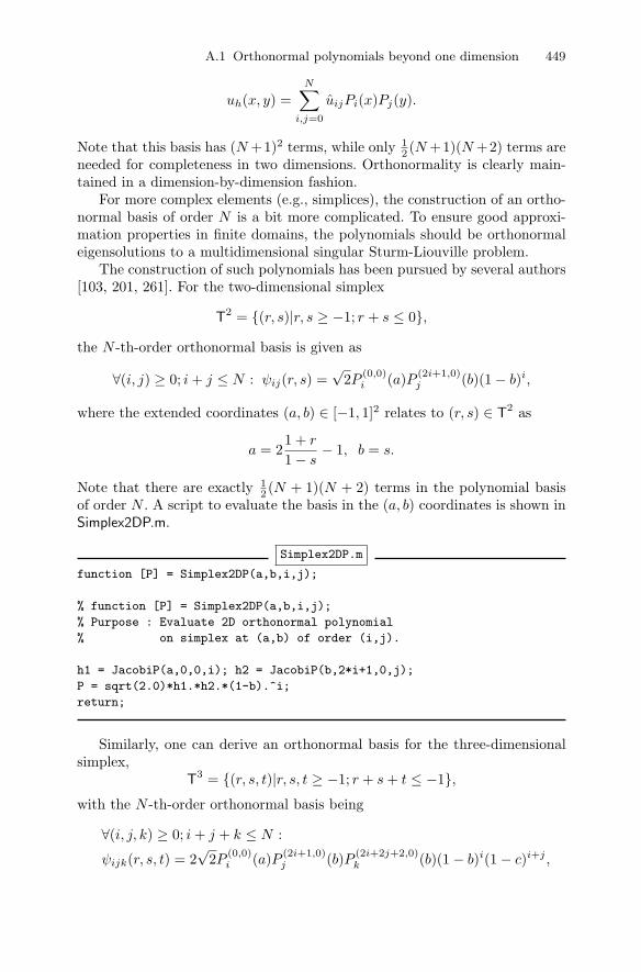
Note that this basis has (N +1)2 terms, while only 12 (N +1)(N +2) terms are
needed for completeness in two dimensions. Orthonormality is clearly main-tained in a dimension-by-dimension fashion.
For more complex elements (e.g., simplices), the construction of an ortho-normal basis of order N is a bit more complicated. To ensure good approxi-mation properties in finite domains, the polynomials should be orthonormaleigensolutions to a multidimensional singular Sturm-Liouville problem.
The construction of such polynomials has been pursued by several authors[103, 201, 261]. For the two-dimensional simplex
T2 = (r, s)|r, s ≥ −1; r + s ≤ 0,
the N -th-order orthonormal basis is given as
∀(i, j) ≥ 0; i + j ≤ N : ψij(r, s) =√
2P(0,0)i (a)P (2i+1,0)
j (b)(1 − b)i,
where the extended coordinates (a, b) ∈ [−1, 1]2 relates to (r, s) ∈ T2 as
a = 21 + r
1 − s− 1, b = s.
Note that there are exactly 12 (N + 1)(N + 2) terms in the polynomial basis
of order N . A script to evaluate the basis in the (a, b) coordinates is shown inSimplex2DP.m.
Simplex2DP.m
function [P] = Simplex2DP(a,b,i,j);
% function [P] = Simplex2DP(a,b,i,j);
% Purpose : Evaluate 2D orthonormal polynomial
% on simplex at (a,b) of order (i,j).
h1 = JacobiP(a,0,0,i); h2 = JacobiP(b,2*i+1,0,j);
P = sqrt(2.0)*h1.*h2.*(1-b).^i;
return;
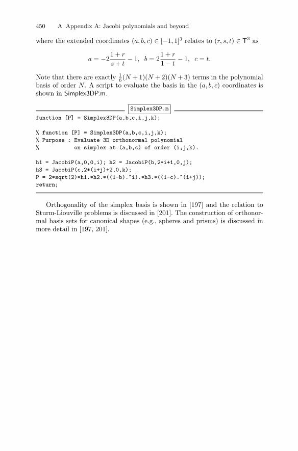
Similarly, one can derive an orthonormal basis for the three-dimensionalsimplex,
T3 = (r, s, t)|r, s, t ≥ −1; r + s + t ≤ −1,with the N -th-order orthonormal basis being
∀(i, j, k) ≥ 0; i + j + k ≤ N :
ψijk(r, s, t) = 2√
2P(0,0)i (a)P (2i+1,0)
j (b)P (2i+2j+2,0)k (b)(1 − b)i(1 − c)i+j ,
450 A Appendix A: Jacobi polynomials and beyond
where the extended coordinates (a, b, c) ∈ [−1, 1]3 relates to (r, s, t) ∈ T3 as
a = −21 + r
s + t− 1, b = 2
1 + r
1 − t− 1, c = t.
Note that there are exactly 16 (N + 1)(N + 2)(N + 3) terms in the polynomial
basis of order N . A script to evaluate the basis in the (a, b, c) coordinates isshown in Simplex3DP.m.
Simplex3DP.m
function [P] = Simplex3DP(a,b,c,i,j,k);
% function [P] = Simplex3DP(a,b,c,i,j,k);
% Purpose : Evaluate 3D orthonormal polynomial
% on simplex at (a,b,c) of order (i,j,k).
h1 = JacobiP(a,0,0,i); h2 = JacobiP(b,2*i+1,0,j);
h3 = JacobiP(c,2*(i+j)+2,0,k);
P = 2*sqrt(2)*h1.*h2.*((1-b).^i).*h3.*((1-c).^(i+j));
return;
Orthogonality of the simplex basis is shown in [197] and the relation toSturm-Liouville problems is discussed in [201]. The construction of orthonor-mal basis sets for canonical shapes (e.g., spheres and prisms) is discussed inmore detail in [197, 201].
B
Appendix B: Briefly on grid generation
by Allan Peter Engsig-Karup
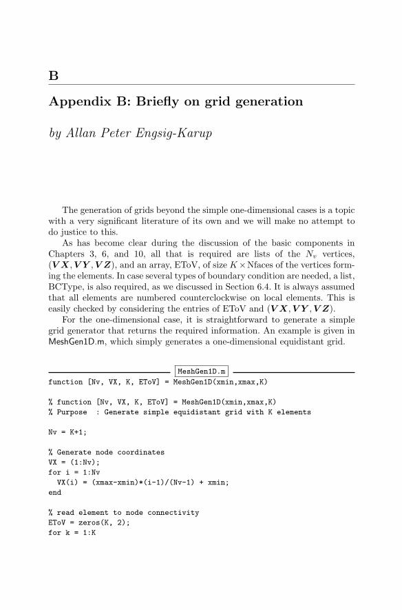
The generation of grids beyond the simple one-dimensional cases is a topicwith a very significant literature of its own and we will make no attempt todo justice to this.
As has become clear during the discussion of the basic components inChapters 3, 6, and 10, all that is required are lists of the Nv vertices,(V X,V Y ,V Z), and an array, EToV, of size K×Nfaces of the vertices form-ing the elements. In case several types of boundary condition are needed, a list,BCType, is also required, as we discussed in Section 6.4. It is always assumedthat all elements are numbered counterclockwise on local elements. This iseasily checked by considering the entries of EToV and (V X,V Y ,V Z).
For the one-dimensional case, it is straightforward to generate a simplegrid generator that returns the required information. An example is given inMeshGen1D.m, which simply generates a one-dimensional equidistant grid.
MeshGen1D.m
function [Nv, VX, K, EToV] = MeshGen1D(xmin,xmax,K)
% function [Nv, VX, K, EToV] = MeshGen1D(xmin,xmax,K)
% Purpose : Generate simple equidistant grid with K elements
Nv = K+1;
% Generate node coordinates
VX = (1:Nv);
for i = 1:Nv
VX(i) = (xmax-xmin)*(i-1)/(Nv-1) + xmin;
end
% read element to node connectivity
EToV = zeros(K, 2);
for k = 1:K
452 B Appendix B: Briefly on grid generation
EToV(k,1) = k; EToV(k,2) = k+1;
end
return
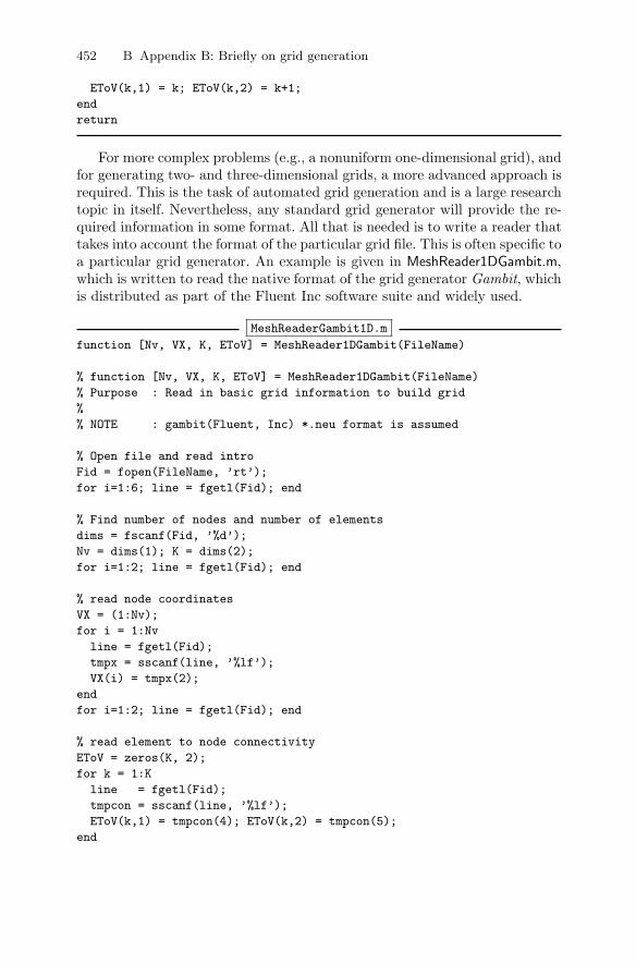
For more complex problems (e.g., a nonuniform one-dimensional grid), andfor generating two- and three-dimensional grids, a more advanced approach isrequired. This is the task of automated grid generation and is a large researchtopic in itself. Nevertheless, any standard grid generator will provide the re-quired information in some format. All that is needed is to write a reader thattakes into account the format of the particular grid file. This is often specific toa particular grid generator. An example is given in MeshReader1DGambit.m,which is written to read the native format of the grid generator Gambit, whichis distributed as part of the Fluent Inc software suite and widely used.
MeshReaderGambit1D.m
function [Nv, VX, K, EToV] = MeshReader1DGambit(FileName)
% function [Nv, VX, K, EToV] = MeshReader1DGambit(FileName)
% Purpose : Read in basic grid information to build grid
%
% NOTE : gambit(Fluent, Inc) *.neu format is assumed
% Open file and read intro
Fid = fopen(FileName, ’rt’);
for i=1:6; line = fgetl(Fid); end
% Find number of nodes and number of elements
dims = fscanf(Fid, ’%d’);
Nv = dims(1); K = dims(2);
for i=1:2; line = fgetl(Fid); end
% read node coordinates
VX = (1:Nv);
for i = 1:Nv
line = fgetl(Fid);
tmpx = sscanf(line, ’%lf’);
VX(i) = tmpx(2);
end
for i=1:2; line = fgetl(Fid); end
% read element to node connectivity
EToV = zeros(K, 2);
for k = 1:K
line = fgetl(Fid);
tmpcon = sscanf(line, ’%lf’);
EToV(k,1) = tmpcon(4); EToV(k,2) = tmpcon(5);
end
B.1 Fundamentals 453
% Close file
st = fclose(Fid);
return
To have a standalone approach, we include here a simple interface and briefdiscussion of the freely available DistMesh software, discussed in detail in
P.O. Persson, G. Strang, A Simple Mesh Generator in MATLAB,SIAM Review, 46(2), 329-345, 2004http://www-math.mit.edu/∼persson/mesh/
This also serves as a more comprehensive user guide. DistMesh is convenientdue to the ease of use and therefore a good starting point before moving onto more complex and advanced applications, which undoubtedly will requiremore advanced mesh generation software.
In the following, we explain how DistMesh can be used to automate theprocess of generating simple uniform and nonuniform meshes in both one andtwo horizontal dimensions. We will provide a few useful scripts and exam-ples on how to setup and define a mesh, how to define the needed boundarymaps from BCType for specifying boundary conditions, using signed distancefunctions to describe the geometries, and how to set up a simple periodicmesh.
B.1 Fundamentals
We illustrate the use of DistMesh to obtain (V X,V Y ) and EToV, needed tocompute connectivities and so forth. DistMesh is based on the use of signeddistance functions to specify geometries. These distance functions can thenbe combined and manipulated to specify whether one is inside or outside aparticular geometry, with negative being inside the geometry.
The general calling sequence for DistMesh is
>> function [p,t] = distmeshnd(fd,fh,h0,bbox,pfix,varargin);
The arguments are
Input The six input variables are
fd Function which returns the signed distance from each node to theboundary.
fh Function which returns the relative edge length for all input points.h0 Initial grid size, which will also be the approximate grid size for an
equidistant grid.bbox Bounding box for the geometry.
454 B Appendix B: Briefly on grid generation
pfix Array of fixed nodes.varargin Optional array with additional parameters to fd and fh if needed.
Output The two output variables are
p List of vertices, i.e., V X=p(:,1)’, V Y =p(:,2)’, etct List of elements, EToV=t.
Let us first consider an example in which we generate a simple one-dimensionalmesh of nonuniform line segments clustered about x = 0 on Ω = [−1, 1]. Wedefine a signed distance function as
% distance function for a circle about xc=0>> fd=inline(’abs(p)-1’,’p’);
where p can be thought of as an x-coordinate. In this case, the distance func-tion can be specified through an inline function, but this is not required.
To specify a nonuniform grid size, we must also specify an element sizefunction that reflects the relative distribution over the domain; that is, thenumbers in this function do not reflect the actual grid size. As an example,consider
% distribution weight function>> fh=inline(’abs(p)*0.075+0.0125’,’p’);
The mesh is now generated through the sequence
% generate non-uniform example mesh in 1D using DistMesh>> h0 = 0.025; % chosen element spacing>> [p,t]=distmeshnd(fd,fh,h0,[-1;1],[]);>> K = size(t,1); Nv = size(p,1);
Two tables are returned that completely defines the mesh and we can findthe number of elements, K, and vertices, Nv, directly from the size of thesearrays.
A uniform mesh can be generated by using the intrinsic function, @huniformas
% generate uniform example mesh in 1D using DistMesh>> [p,t]=distmeshnd(fd,@huniform,h0,[-1;1],[]);
The vertex nodes are sorted to be in ascending order as
>> [x,i]=sort(p(t));>> t=t(i,:);>> t=sort(t’,’ascend’)’;>> EToV = t; VX = p(:,1)’;
B.1 Fundamentals 455
This can now be returned directly to the solver. These simple steps are allcollected in the small script MeshGenDistMesh1D.m.
MeshGenDistMesh1D.m
function [Nv, VX, K, EToV] = MeshGenDistMesh1D()
% function [VX, K, EToV] = MeshGenDistMesh1D()
% Purpose : Generate 1D mesh using DistMesh;
% distance function for a circle about xc=0
fd=inline(’abs(p)-1’,’p’);
% distribution weight function
fh=inline(’abs(p)*0.075+0.0125’,’p’);
% generate non-uniform example mesh in 1D using DistMesh
h0 = 0.025; % chosen element spacing
[p,t]=distmeshnd(fd,fh,h0,[-1;1],[]);
K = size(t,1); Nv = K+1;
% Sort elements in ascending order
[x,i]=sort(p(t));
t=t(i,:);
Met=sort(t’,’ascend’)’;
EToV = t; VX = p(:,1)’;
return
Two-dimensional grids can be created in a similar way. Consider as an ex-ample the need to generate an equidistant grid in a circular domain, boundedby [−1, 1]2. Following the outline above, we continue as
>> fd = inline(’sqrt(sum(p.∧2,2))-1’,’p’);>> [p,t] = distmeshnd(fd,@huniform,0.2,[-1 -1; 1 1], []);>> VX = p(:,1)’; VY = p(:,2)’;>> K = size(t,1); Nv = size(p,1);>> EToV = t;
Note, that DistMesh does not guarantee a counterclockwise ordering of theelement vertices and we therefore check and correct all element orderings toensure this. This can be done in various ways; for example,
>> ax = VX(EToV(:,1)); ay = VY(EToV(:,1));>> bx = VX(EToV(:,2)); by = VY(EToV(:,2));>> cx = VX(EToV(:,3)); cy = VY(EToV(:,3));>> D = (ax-cx).*(by-cy)-(bx-cx).*(ay-cy);>> i = find(D<0);>> EToV(i,:) = EToV(i,[1 3 2]);
456 B Appendix B: Briefly on grid generation
There are many more examples in the DistMesh user guide where one alsocan find a list of a variety of simple functions; for example, to create two-dimensional rectangular grids, one can use
>> fd = inline(’drectangle(p,-1,1,-1,1)’,’p’);>>[p,t] = distmeshnd(fd,@huniform,0.2,[-1 -1; 1 1], []);>> VX = p(:,1)’; VY = p(:,2)’;>> K = size(t,1); Nv = size(p,1);>> EToV = t;
possibly followed by sorting as needed. The process is illustrated in Mesh-GenDistMesh2D.m.
MeshGenDistMesh2D.m
function [VX, VY, K, EToV] = MeshGenDistMesh2D()
% function [VX, VY, K, EToV] = MeshGenDistMesh2D()
% Purpose : Generate 2D square mesh using DistMesh;
% By Allan P. Engsig-Karup
% Parameters to set/define
% fd Distance function for mesh boundary
% fh Weighting function for distributing elements
% h0 Characteristic length of elements
% Bbox Bounding box for mesh
% param Parameters to be used in function call with DistMesh
fd = inline(’drectangle(p,-1,1,-1,1)’,’p’);
fh = @huniform;
h0 = 0.25;
Bbox = [-1 -1; 1 1];
param = [];
% Call distmesh
[Vert,EToV]=distmesh2d(fd,fh,h0,Bbox,param);
VX = Vert(:,1)’; VY = Vert(:,2)’;
Nv = length(VX); K = size(EToV,1);
% Reorder elements to ensure counter clockwise orientation
ax = VX(EToV(:,1)); ay = VY(EToV(:,1));
bx = VX(EToV(:,2)); by = VY(EToV(:,2));
cx = VX(EToV(:,3)); cy = VY(EToV(:,3));
D = (ax-cx).*(by-cy)-(bx-cx).*(ay-cy);
i = find(D<0);
EToV(i,:) = EToV(i,[1 3 2]);
return
B.2 Creating boundary maps 457
B.2 Creating boundary maps
While many examples and general grids are shown in the DistMesh user guide,the creation of special boundary maps for imposing different boundary con-ditions requires a few more steps.
A boundary table for all element faces is easily obtained from the EToEarray as
>> BCType = int8(not(EToE));
However, if we want to be able to distinguish the different boundaries, we needan efficient way to specify boundary properties. This can conveniently be doneusing a distance function with the properties that d = 0 on the boundary andd <> 0 outside the boundary.
Let us consider an example. We set up a unit circle with a hole in themiddle as
>> fd=inline(’-0.3+abs(0.7-sqrt(sum(p.∧2,2)))’);>> [p,t]=distmeshnd(fd,@huniform,0.1,[-1,-1;1,1],[]);
which is easily generated with two lines of code using DistMesh.We wish to define two maps mapI and mapO that allow us to specify
different boundary conditions on the inner and the outer boundary of the unitcircle with a hole. We note that the following distance functions describe theboundaries completely (as sketched in Fig. B.1):
>> fd inner=inline(’sqrt(sum(p.∧2,2))-0.4’,’p’);>> fd outer=inline(’sqrt(sum(p.∧2,2))-1’,’p’);
Using these functions, we can determine index lists of the vertex nodes onthe boundaries by
>> tol = 1e-8; % tolerance level used for determining nodes>> nodesInner = find( abs(fd inner(p))<tol );>> nodesOuter = find( abs(fd outer(p))<tol );
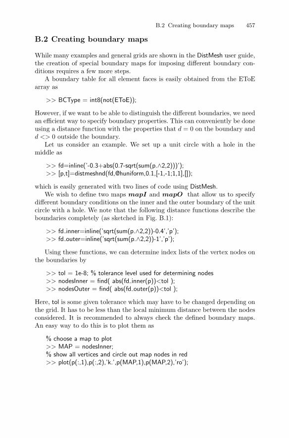
Here, tol is some given tolerance which may have to be changed depending onthe grid. It has to be less than the local minimum distance between the nodesconsidered. It is recommended to always check the defined boundary maps.An easy way to do this is to plot them as
% choose a map to plot>> MAP = nodesInner;% show all vertices and circle out map nodes in red>> plot(p(:,1),p(:,2),’k.’,p(MAP,1),p(MAP,2),’ro’);
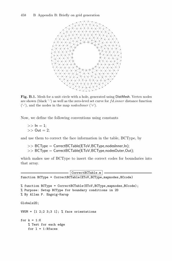
458 B Appendix B: Briefly on grid generation
Fig. B.1. Mesh for a unit circle with a hole, generated using DistMesh. Vertex nodesare shown (black ’·’) as well as the zero-level set curve for fd inner distance function(’-’), and the nodes in the map nodesInner (’’).
Now, we define the following conventions using constants
>> In = 1;>> Out = 2;
and use them to correct the face information in the table, BCType, by
>> BCType = CorrectBCTable(EToV,BCType,nodesInner,In);>> BCType = CorrectBCTable(EToV,BCType,nodesOuter,Out);
which makes use of BCType to insert the correct codes for boundaries intothat array.
CorrectBCTable.m
function BCType = CorrectBCTable(EToV,BCType,mapnodes,BCcode)
% function BCType = CorrectBCTable(EToV,BCType,mapnodes,BCcode);
% Purpose: Setup BCType for boundary conditions in 2D
% By Allan P. Engsig-Karup
Globals2D;
VNUM = [1 2;2 3;3 1]; % face orientations
for k = 1:K
% Test for each edge
for l = 1:Nfaces
B.2 Creating boundary maps 459
m = EToV(k,VNUM(l,1)); n = EToV(k,VNUM(l,2));
% if both points are on the boundary then it is a boundary
% point!
ok=sum(ismember([m n],mapnodes));
if ok==2
BCType(k,l)=BCcode;
end;
end
end
return
Once this is generated, one can follow the discussion in Section 6.4 tocreate the appropriate boundary maps. The creation of special boundary mapsis illustrated using the script ConstructMap.m after having corrected the faceinformation of BCType.
% Construct special face from the BCType table>> mapI = ConstructMap(BCType, In);>> mapO = ConstructMap(BCType, Out);
ConstructMap.m
function [map] = ConstructMap(BCType, BCcode)
% function map = ConstructMap(BCType, BCcode);
% Purpose: Construct boundary map from the BCType table
% By Allan P. Engsig-Karup, 07-12-2006.
Globals2D;
% Determine which faces in which elements which have the specified BCs:
% fids = face id’s, eids = element id’s;
[eids,fids] = find(BCType==BCcode);
% initialize length of new map
map = [];
for n = 1 : length(fids) % go over each boundary face of BCcode type
map = [map (eids(n)-1)*Nfaces*Nfp+[ (fids(n)-1)*Nfp + [1:Nfp] ]];
end
return
C
Appendix C: Software, variables,and helpful scripts
All codes discussed in this text can be downloaded freely at
http://www.nudg.org
The codes are distributed with the following disclaimer:
Permission to use this software for noncommercialresearch and educational purposes is hereby grantedwithout fee. Redistribution, sale, or incorporationof this software into a commercial product is prohibited.
THE AUTHORS OR PUBLISHER DISCLAIMS ANY AND ALL WARRANTIESWITH REGARD TO THIS SOFTWARE,INCLUDING ALL IMPLIEDWARRANTIES OF MERCHANTABILITY AND FITNESS FOR ANYPARTICULAR PURPOSE. IN NO EVENT SHALL THE AUTHORS ORTHE PUBLISHER BE LIABLE FOR ANY SPECIAL, INDIRECT ORCONSEQUENTIAL DAMAGES OR ANY DAMAGES WHATSOEVERRESULTING FROM LOSS OF USE, DATA OR PROFITS.
C.1 List of important variables defined in the codes
In the following, we list the basic parameters and arrays used in the codesdiscussed throughout. This is done to help users understand the notation andenable them to quickly alter the codes to suit their needs. Note that the listis not exhaustive and only the essential parameters, arrays, and operators areincluded.
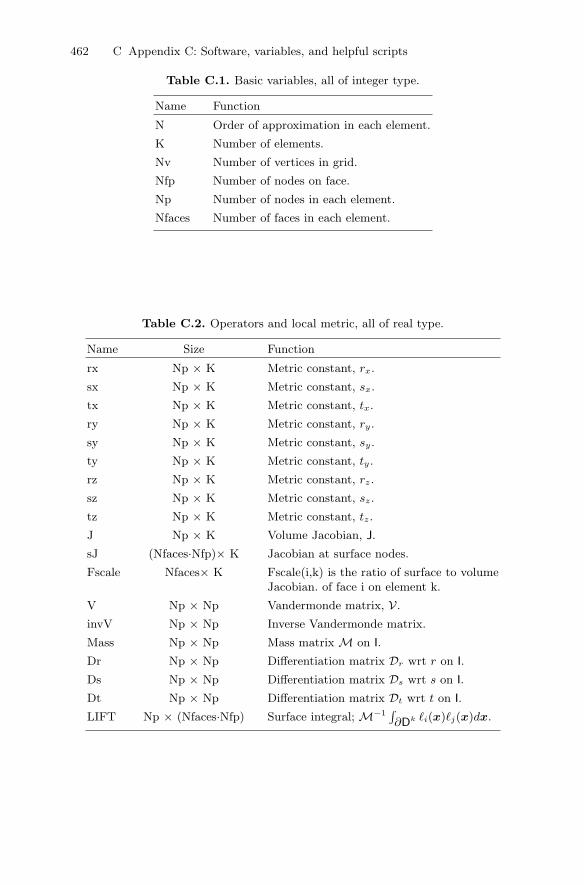
462 C Appendix C: Software, variables, and helpful scripts
Table C.1. Basic variables, all of integer type.
Name Function
N Order of approximation in each element.
K Number of elements.
Nv Number of vertices in grid.
Nfp Number of nodes on face.
Np Number of nodes in each element.
Nfaces Number of faces in each element.
Table C.2. Operators and local metric, all of real type.
Name Size Function
rx Np × K Metric constant, rx.
sx Np × K Metric constant, sx.
tx Np × K Metric constant, tx.
ry Np × K Metric constant, ry.
sy Np × K Metric constant, sy.
ty Np × K Metric constant, ty.
rz Np × K Metric constant, rz.
sz Np × K Metric constant, sz.
tz Np × K Metric constant, tz.
J Np × K Volume Jacobian, J.
sJ (Nfaces·Nfp)× K Jacobian at surface nodes.
Fscale Nfaces× K Fscale(i,k) is the ratio of surface to volumeJacobian. of face i on element k.
V Np × Np Vandermonde matrix, V.
invV Np × Np Inverse Vandermonde matrix.
Mass Np × Np Mass matrix M on I.
Dr Np × Np Differentiation matrix Dr wrt r on I.
Ds Np × Np Differentiation matrix Ds wrt s on I.
Dt Np × Np Differentiation matrix Dt wrt t on I.
LIFT Np × (Nfaces·Nfp) Surface integral; M−1∫∂Dk i(x)j(x)dx.
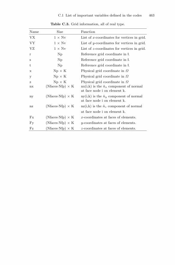
C.1 List of important variables defined in the codes 463
Table C.3. Grid information, all of real type.
Name Size Function
VX 1 × Nv List of x-coordinates for vertices in grid.
VY 1 × Nv List of y-coordinates for vertices in grid.
VZ 1 × Nv List of z-coordinates for vertices in grid.
r Np Reference grid coordinate in I.
s Np Reference grid coordinate in I.
t Np Reference grid coordinate in I.
x Np × K Physical grid coordinate in Ω
y Np × K Physical grid coordinate in Ω
z Np × K Physical grid coordinate in Ωnx (Nfaces·Nfp) × K nx(i,k) is the nx component of normal
at face node i on element k.
ny (Nfaces·Nfp) × K ny(i,k) is the ny component of normalat face node i on element k.
nz (Nfaces·Nfp) × K nz(i,k) is the nz component of normal
at face node i on element k.
Fx (Nfaces·Nfp) × K x-coordinates at faces of elements.
Fy (Nfaces·Nfp) × K y-coordinates at faces of elements.
Fz (Nfaces·Nfp) × K z-coordinates at faces of elements.
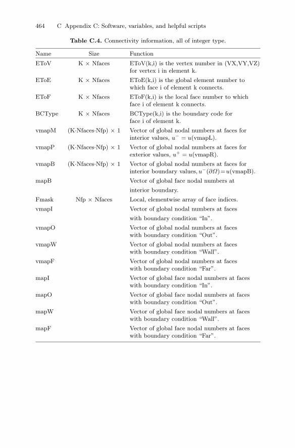
464 C Appendix C: Software, variables, and helpful scripts
Table C.4. Connectivity information, all of integer type.
Name Size Function
EToV K × Nfaces EToV(k,i) is the vertex number in (VX,VY,VZ)for vertex i in element k.
EToE K × Nfaces EToE(k,i) is the global element number towhich face i of element k connects.
EToF K × Nfaces EToF(k,i) is the local face number to whichface i of element k connects.
BCType K × Nfaces BCType(k,i) is the boundary code forface i of element k.
vmapM (K·Nfaces·Nfp) × 1 Vector of global nodal numbers at faces forinterior values, u− = u(vmapL).
vmapP (K·Nfaces·Nfp) × 1 Vector of global nodal numbers at faces forexterior values, u+ = u(vmapR).
vmapB (K·Nfaces·Nfp) × 1 Vector of global nodal numbers at faces forinterior boundary values, u−(∂Ω)=u(vmapB).
mapB Vector of global face nodal numbers at
interior boundary.
Fmask Nfp × Nfaces Local, elementwise array of face indices.
vmapI Vector of global nodal numbers at faces
with boundary condition “In”.
vmapO Vector of global nodal numbers at faceswith boundary condition “Out”.
vmapW Vector of global nodal numbers at faceswith boundary condition “Wall”.
vmapF Vector of global nodal numbers at faceswith boundary condition “Far”.
mapI Vector of global face nodal numbers at faceswith boundary condition “In”.
mapO Vector of global face nodal numbers at faceswith boundary condition “Out”.
mapW Vector of global face nodal numbers at faceswith boundary condition “Wall”.
mapF Vector of global face nodal numbers at faceswith boundary condition “Far”.
C.2 List of additional useful scripts 465
C.2 List of additional useful scripts
In the following, we provide a number of Matlab scripts that are not discussedas part of the text, but nevertheless prove useful when developing algorithmsand visualizing the computed results.
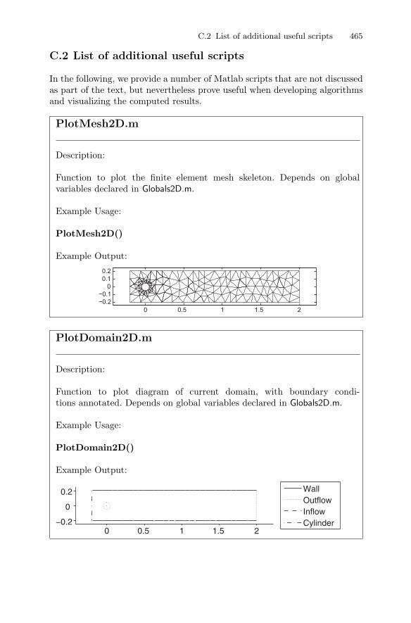
PlotMesh2D.m
Description:
Function to plot the finite element mesh skeleton. Depends on globalvariables declared in Globals2D.m.
Example Usage:
PlotMesh2D()
Example Output:
0 0.5 1 1.5 2−0.2−0.1
00.10.2
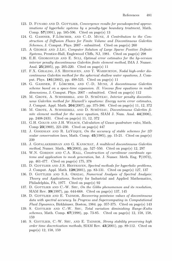
PlotDomain2D.m
Description:
Function to plot diagram of current domain, with boundary condi-tions annotated. Depends on global variables declared in Globals2D.m.
Example Usage:
PlotDomain2D()
Example Output:
0 0.5 1 1.5 2−0.2
0
0.2 WallOutflowInflowCylinder
466 C Appendix C: Software, variables, and helpful scripts
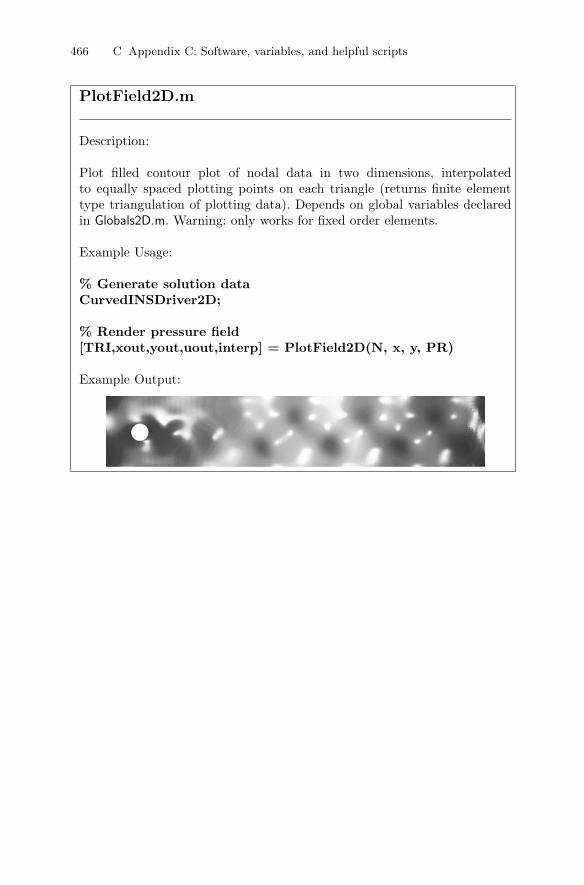
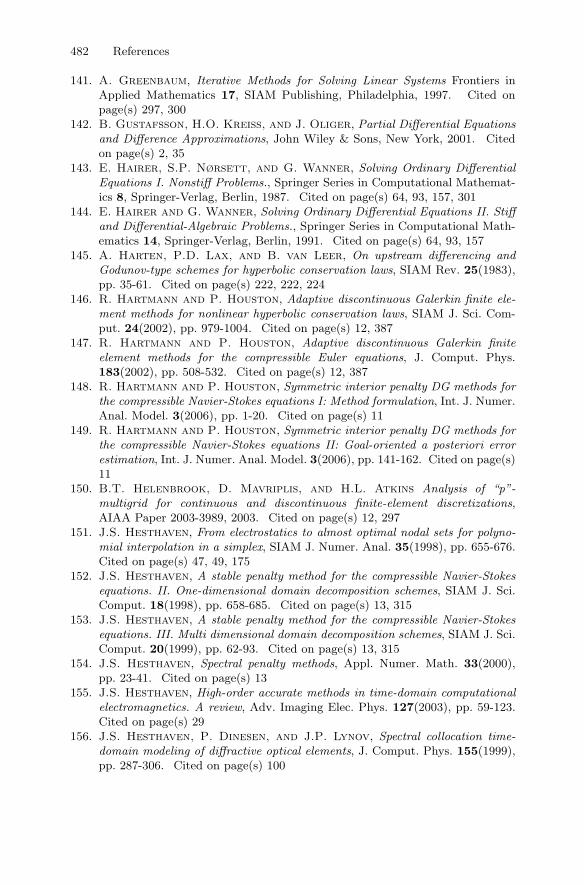
PlotField2D.m
Description:
Plot filled contour plot of nodal data in two dimensions, interpolatedto equally spaced plotting points on each triangle (returns finite elementtype triangulation of plotting data). Depends on global variables declaredin Globals2D.m. Warning: only works for fixed order elements.
Example Usage:
% Generate solution dataCurvedINSDriver2D;
% Render pressure field[TRI,xout,yout,uout,interp] = PlotField2D(N, x, y, PR)
Example Output:
C.2 List of additional useful scripts 467
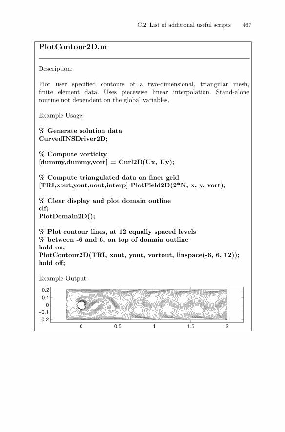
PlotContour2D.m
Description:
Plot user specified contours of a two-dimensional, triangular mesh,finite element data. Uses piecewise linear interpolation. Stand-aloneroutine not dependent on the global variables.
Example Usage:
% Generate solution dataCurvedINSDriver2D;
% Compute vorticity[dummy,dummy,vort] = Curl2D(Ux, Uy);
% Compute triangulated data on finer grid[TRI,xout,yout,uout,interp] PlotField2D(2*N, x, y, vort);
% Clear display and plot domain outlineclf;PlotDomain2D();
% Plot contour lines, at 12 equally spaced levels% between -6 and 6, on top of domain outlinehold on;PlotContour2D(TRI, xout, yout, vortout, linspace(-6, 6, 12));hold off;
Example Output:
0 0.5 1 1.5 2−0.2−0.1
00.10.2
468 C Appendix C: Software, variables, and helpful scripts
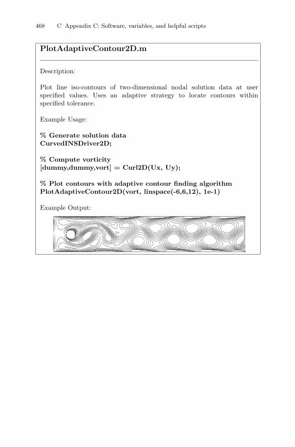
PlotAdaptiveContour2D.m
Description:
Plot line iso-contours of two-dimensional nodal solution data at userspecified values. Uses an adaptive strategy to locate contours withinspecified tolerance.
Example Usage:
% Generate solution dataCurvedINSDriver2D;
% Compute vorticity[dummy,dummy,vort] = Curl2D(Ux, Uy);
% Plot contours with adaptive contour finding algorithmPlotAdaptiveContour2D(vort, linspace(-6,6,12), 1e-1)
Example Output:
C.2 List of additional useful scripts 469
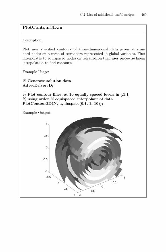
PlotContour3D.m
Description:
Plot user specified contours of three-dimensional data given at stan-dard nodes on a mesh of tetrahedra represented in global variables. Firstinterpolates to equispaced nodes on tetrahedron then uses piecewise linearinterpolation to find contours.
Example Usage:
% Generate solution dataAdvecDriver3D;
% Plot contour lines, at 10 equally spaced levels in [.1,1]% using order N equispaced interpolant of dataPlotContour3D(N, u, linspace(0.1, 1, 10));
Example Output:
470 C Appendix C: Software, variables, and helpful scripts
PlotAdaptiveContour3D.m
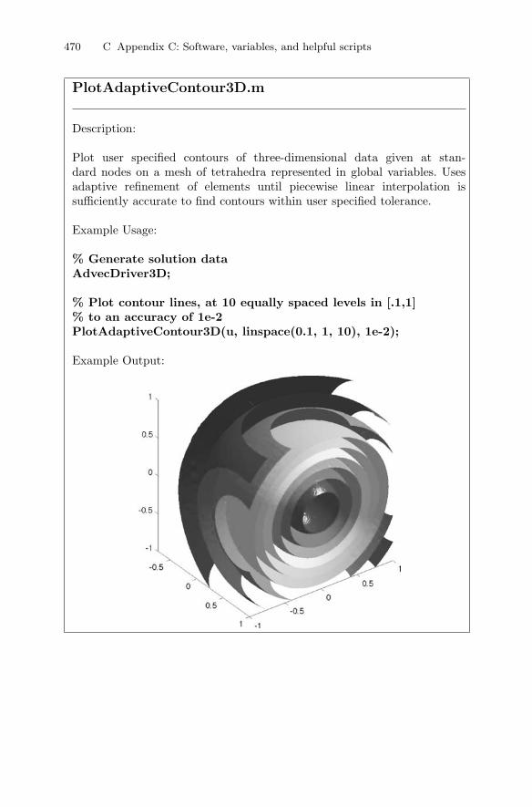
Description:
Plot user specified contours of three-dimensional data given at stan-dard nodes on a mesh of tetrahedra represented in global variables. Usesadaptive refinement of elements until piecewise linear interpolation issufficiently accurate to find contours within user specified tolerance.
Example Usage:
% Generate solution dataAdvecDriver3D;
% Plot contour lines, at 10 equally spaced levels in [.1,1]% to an accuracy of 1e-2PlotAdaptiveContour3D(u, linspace(0.1, 1, 10), 1e-2);
Example Output:
C.2 List of additional useful scripts 471
PlotSlice3D.m
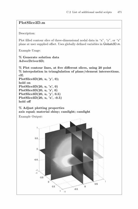
Description:
Plot filled contour slice of three-dimensional nodal data in “x”, “y”, or “z”plane at user supplied offset. Uses globally defined variables in Globals3D.m.
Example Usage:
% Generate solution dataAdvecDriver3D;
% Plot contour lines, at five different slices, using 20 point% interpolation in trianglulation of plane/element intersections.clf;PlotSlice3D(20, u, ’y’, 0);hold onPlotSlice3D(20, u, ’x’, 0)PlotSlice3D(20, u, ’z’, 0)PlotSlice3D(20, u, ’y’, 0.5)PlotSlice3D(20, u, ’x’, -0.5)hold off
% Adjust plotting propertiesaxis equal; material shiny; camlight; camlight
Example Output:
References
1. S. Abarbanel and A. Ditkowski, Asymptotically stable fourth-order accu-rate schemes for the diffusion equation on complex shapes, J. Comput. Phys.133(1997), pp. 279-288. Cited on page(s) 13
2. S. Abarbanel and D. Gottlieb, On the construction and analysis of ab-sorbing layers in CEM, Appl. Numer. Math. 27(1998), pp. 331-340. Cited onpage(s) 240
3. R. Abgrall and H. Deconinck (Eds.), Comput. Fluids 34(4-5), 2005. Citedon page(s) 13
4. M. Abromowitz and I.A. Stegun (Eds.), Handbook of Mathematical Func-tions, Dover Publications, New York, 1972. Cited on page(s) 446
5. S. Adjerid and M. Baccouch, The discontinuous Galerkin method for two-dimensional hyperbolic problems. Part I: Superconvergence error analysis,J. Sci. Comput. 33(2007), pp. 75-113. Cited on page(s) 12, 396
6. S. Adjerid, K. Devine, J. Flaherty, and L. Krivodonova, A posteriorierror estimation for discontinuous Galerkin solutions of hyperbolic problems,Comput. Methods Appl. Mech. Eng. 191(2002), pp. 1097-1112. Cited onpage(s) 12, 387, 396
7. S. Adjerid and T.C. Massey, A posteriori discontinuous finite element errorestimation for two-dimensional hyperbolic problems, Comput. Methods Appl.Mech. Eng. 191(2002), pp. 5877-5897. Cited on page(s) 12, 387
8. S. Adjerid and T.C. Massey, Superconvergence of discontinuous finite el-ement solutions for nonlinear scalar hyperbolic problems Comput. MethodsAppl. Mech. Eng. 195(2006), pp. 3331-3346. Cited on page(s) 12, 387
9. M. Ainsworth, Dispersive and dissipative behavior of high-order discontinuousGalerkin finite element methods, J. Comput. Phys. 198(2002), pp. 106-130.Cited on page(s) 91, 91, 92, 92
10. M. Ainsworth, P. Monk, and W. Muniz, Dispersive and dissipative prop-erties of discontinuous Galerkin finite element methods for the second-orderwave equation, J. Sci. Comput. 27(2006), pp. 5-40. Cited on page(s) 93, 353
11. P.F. Antonietti, A. Buffa, and I. Perugia, Discontinuous Galerkin ap-proximation of the Laplace eigenproblem, Comput. Methods Appl. Mech. Eng.195(2006), pp. 3483-3503. Cited on page(s) 12, 337, 338, 338, 338
474 References
12. D.N. Arnold, An interior penalty finite element method with discontinuouselements, SIAM J. Numer. Anal. 19(1982), pp. 724-760. Cited on page(s) 11,11, 282, 296
13. D.N. Arnold, F. Brezzi, B. Cockburn, and L.D. Marini, Unified analysisof discontinuous Galerkin methods for elliptic problems, SIAM J. Numer. Anal.39(2002), pp. 1749-1779. Cited on page(s) 11, 270, 282, 288, 292, 293, 296,296
14. H. Atkins and C.-W. Shu, Quadrature-free implementation of the discontin-uous Galerkin method for hyperbolic equations, AIAA J. 36(1998), pp. 775-782.Cited on page(s) 11, 211
15. I. Babuska and M.R. Dorr, Error estimates for the combined h- andp-versions of the finite element method, Numer. Math. 37(1981), pp. 257-277.Cited on page(s) 387, 396
16. I. Babuska, B.A. Szabo, and I.N. Katz, The p-version of the finite elementmethod, SIAM J. Numer. Anal. 18(1981), pp. 515-545. Cited on page(s) 387
17. I. Babuska and B. Guo, The h-p version of the finite element method - Part 1:The basic approximation results, Comput. Mech. 1(1986), pp. 21-41. Cited onpage(s) 387
18. I. Babuska and B. Guo, The h-p version of the finite element method - Part 2:General results and applications, Comput. Mech. 1(1986), pp. 203-220. Citedon page(s) 387
19. I. Babuska and T. Strouboulis, The Finite Element Method and its Re-liability, Oxford University Press, Oxford, 2001. Cited on page(s) 293, 387,396
20. F. Bassi, A. Crivellini, S. Rebay, and M. Savini, Discontinuous Galerkinsolution of the Reynolds-averaged NavierStokes and kω turbulence model equa-tions, Comput. Fluids 34(2005), pp. 507-540. Cited on page(s) 316
21. F. Bassi and S. Rebay, A high-order discontinuous Galerkin finite elementmethod solution of the 2D Euler equations, J. Comput. Phys. 138(1997),pp. 251-285. Cited on page(s) 11, 316, 320, 375
22. F. Bassi and S. Rebay, A high-order accurate discontinuous Galerkin finiteelement method for the numerical solution of the compressible Navier-Stokesequations, J. Comput. Phys. 131(1997), pp. 267-279. Cited on page(s) 11, 11,11, 245, 315
23. F. Bassi and S. Rebay, Numerical evaluation of two discontinuous Galerkinmethods for the compressible Navier-Stokes equations, Int. J. Numer. MethodsFluids 40(2002), pp. 197-207. Cited on page(s) 315
24. C.E. Baumann and J.T. Oden, A discontinuous hp-Finite element method forconvection-diffusion problems, Comput. Methods Appl. Mech. Eng. 175(1999),pp. 311-341. Cited on page(s) 11
25. J.P. Berenger, A perfectly matched layer for the absorption of electromag-netic waves, J. Comput. Phys. 114(1994), pp. 185-200. Cited on page(s) 240
26. J.P. Berenger, Three-dimensional perfectly matched layer for the absorptionof electromagnetic waves, J. Comput. Phys. 127(1996), pp. 363-379. Cited onpage(s) 240
27. C. Bernardi and Y. Maday, Polynomial interpolation results in Sobolevspaces, J. Comput. Appl. Math. 43(1992), pp. 53-80. Cited on page(s) 81,82
References 475
28. R. Biswas, K.D. Devine, and J. Flaherty, Parallel, adaptive finite elementmethods for conservation laws, Appl. Numer. Math. 14(1994), pp. 255-283.Cited on page(s) 12, 156, 387, 396
29. D. Boffi, R.G. Duran, and L. Gastaldi, A remark on spurious eigenvaluesin a square, Appl. Math. Lett. 12(1999), pp. 107-114. Cited on page(s) 333
30. D. Boffi. M. Farina, and L. Gastaldi, On the approximation of Maxwell’seigenproblem in general 2D domains, Comput. Struct. 79(2001), pp. 1089-1096.Cited on page(s) 333
31. F. van ded Bos, J.J.W. van der Vegt, and B. J. Geurts, A multi-scaleformulation for compressible turbulent flows suitable for general variationaldiscretization techniques, Comput. Methods Appl. Mech. Eng. 196(2007),pp. 2863-2875. Cited on page(s) 316
32. F. Brezzi, B. Cockburn, D.M. Marini, and E. Suli, Stabilization mech-anisms in discontinuous Galerkin finite element methods, Comput. MethodsAppl. Mech. Eng. 195(2006), pp. 3293-3310. Cited on page(s) 11
33. F. Brezzi, L.D. Marini, and E. Suli, Discontinuous Galerkin methodsfor first-order hyperbolic problems, M3AS: Math. Models Methods Appl. Sci.14(2004), pp. 1893–1903, 2004. Cited on page(s) 10
34. A. Buffa, P. Houston, and I. Perugia, Discontinuous Galerkin computa-tion of the Maxwell eigenvalues on simplicial meshes, J. Comput. Appl. Math.204(2007), pp. 317-333. Cited on page(s) 12, 348, 370
35. A. Buffa and I. Perugia, Discontinuous Galerkin approximation of theMaxwell eigenproblem, SIAM J. Numer. Anal. 44(2006), pp. 2198-2226. Citedon page(s) 12, 351, 370
36. A. Burbeau, P. Sagaut, and C.-H. Bruneau, A problem-independent lim-iter for high-order Runge-Kutta discontinuous Galerkin methods J. Comput.Phys. 163(2001), pp. 111-150. Cited on page(s) 224
37. A. Burbeau and P. Sagaut, Simulation of a viscous compressible flow pasta circular cylinder with high-order discontinuous Galerkin methods, Comput.Fluids 31(2002), pp. 867-889. Cited on page(s) 315
38. A. Burbeau and P. Sagaut, A dynamic p-adaptive Discontinuous Galerkinmethod for viscous flow with shocks, Comput. Fluids 34(2005), pp. 401-417.Cited on page(s) 315
39. E. Burman and B. Stamm, Minimal stabilization for discontinuous Galerkinfinite element methods for hyperbolic problems, J. Sci. Comput. 33(2007(),pp. 183-208. Cited on page(s) 10, 33
40. J.C. Butcher, The Numerical Analysis of Ordinary Differential Equations:Runge-Kutta and General Linear Methods, John Wiley & Sons, New York,2003. Cited on page(s) 64, 93, 101, 157
41. N. Canouet, L. Fezoui, and S. Piperno, Discontinuous Galerkin time-domain solution of Maxwell’s equations on locally-refined nonconformingCartesian grids, COMPEL 24(2005), pp. 1381-1401. Cited on page(s) 110
42. C. Canuto, M.Y. Hussaini, A. Quarteroni, and T.A. Zang, Spec-tral Methods in Fluid Dynamics, Springer Series in Computational Physics,Springer-Verlag, New York, 1988. Cited on page(s) 186
43. C. Canuto and A. Quarteroni, Approximation results for orthogonal poly-nomials in Sobolev spaces, Math. Comp. 38(1982), pp. 67-86. Cited on page(s)79, 79, 79
476 References
44. M.H. Carpenter, D. Gottlieb, and S. Abarbanel, Time-stable boundaryconditions for finite-difference schemes solving hyperbolic systems: Methodologyand application to high-order compact schemes, J. Comput. Phys. 111(1994),pp. 220-236. Cited on page(s) 13
45. M.H. Carpenter, D. Gottlieb, and C.-W. Shu, On the conservation andconvergence to weak solutions of global schemes, J. Sci. Comput. 18(2003),pp. 111-132. Cited on page(s) 120, 134
46. M.H. Carpenter and C. Kennedy, Fourth-order 2N-storage Runge-Kuttaschemes, NASA Report TM 109112, NASA Langley Research Center, 1994.Cited on page(s) 64
47. M.H. Carpenter, J. Nordstrom, and D. Gottlieb A stable and con-servative interface treatment of arbitrary spatial accuracy, J. Comput. Phys.148(1999), pp. 341-365. Cited on page(s) 13
48. P. Castillo, Performance of discontinuous Galerkin methods for elliptic prob-lems, SIAM J. Sci. Comput. 24(2002), pp. 524-547. Cited on page(s) 11, 11,270
49. P. Castillo, A review of the local discontinuous Galerkin (LDG) method ap-plied to elliptic problems, Appl. Numer. Math. 56(2006), pp. 1307-1313. Citedon page(s) 270
50. P. Castillo, B. Cockburn, I. Perugia, and D. Schotzau, An a priorierror analysis of the local discontinuous Galerkin method for elliptic problemsSIAM J. Numer. Anal. 38(2000), pp. 1676-1706. Cited on page(s) 11, 296
51. P. Castillo, B. Cockburn, D. Schotzau, and C. Schwab, Optimal apriori error estimates for the hp-version of the local discontinuous Galerkinmethod for convection-diffusion problems, Math. Comp. 71(2002), pp. 455-478.Cited on page(s) 11
52. C. Chauviere, J. S. Hesthaven, A. Kanevsky, and T. Warburton, High-order localized time integration for grid-induced stiffness, 2nd MIT Conferenceon Fluid Dynamics, Boston. Vol. II, pp. 1883-1886, 2003. Cited on page(s)110
53. G. Chavent and G. Salzano, A finite element method for the 1D floodingproblem with gravity, J. Comput. Phys. 45(1982), pp. 307-344. Cited on page(s)10
54. G. Chavent and B. Cockburn, The local projection p0-p1-discontinuousGalerkin finite element for scalar conservation laws, M2AN 23(1989), pp. 565-592. Cited on page(s) 10
55. Q. Chen and I. Babuska, Approximate optimal points for polynomial inter-polation of real functions in an interval and in a triangle, Comput. Meth. inApp. Mech. and Eng. 128(1995), pp. 405–417. Cited on page(s) 175, 412, 414,414
56. Y. Cheng and C.-W. Shu, A discontinuous Galerkin finite element method fordirectly solving the Hamilton-Jacobi equations, J. Comput. Phys. 223(2007),pp. 398-415. Cited on page(s) 11, 135
57. Y. Cheng and C.-W. Shu, A discontinuous Galerkin finite element methodfor time dependent partial differential equations with higher order derivatives,Math. Comp 2007 – to appear. Cited on page(s) 260, 261, 261
58. E.T. Chung and B. Engquist, Optimal discontinuous Galerkin methods forwave propagation, SIAM J. Sci. Comput. 44(2006), pp. 2131-2158. Cited onpage(s) 11
References 477
59. P.G. Ciarlet, The Finite Element Method for Elliptic Problems, SIAM Clas-sic in Applied Mathematics 40, SIAM Publications, Philadelphia, 2002. Citedon page(s) 87, 87, 261, 287, 292
60. B. Cockburn, Discontinuous Galerkin method for convection-dominated Prob-lems. In High-Order Methods for Computational Physics, T.J. Barth and H.Deconinck (Eds.), Lecture Notes in Computational Science and Engineering 9,Springer-Verlag, Berlin, pp. 69-224, 1999. Cited on page(s) 88, 88, 145, 148,152, 161
61. B. Cockburn and B. Dong, An analysis of the minimal dissipation local dis-continuous Galerkin method for convection diffusion problems. J. Sci. Comput.32(2007), pp. 233-262. Cited on page(s) 10, 33
62. B. Cockburn and P.A. Gremaud, Error estimates for finite element methodsfor nonlinear conservation laws, SIAM J. Numer. Anal. 33(1996), pp. 522-554.Cited on page(s) 12, 387
63. B. Cockburn and J. Guzman, Error estimates for the Runge-Kutta discon-tinuous Galerkin method for the transport equation with discontinuous initialdata, SIAM J. Numer. Anal. 2007 – submitted. Cited on page(s) 10
64. B. Cockburn, S. Hou, and C.-W. Shu, TVB Runge-Kutta local projectiondiscontinuous Galerkin finite element method for conservation laws IV: Themultidimensional case, Math. Comp. 54(1990), pp. 545-581. Cited on page(s)10, 224, 239
65. B. Cockburn, G. Kanschat, I. Perugia, and D. Schotzau, Supercon-vergence of the local discontinuous Galerkin method for elliptic problems onCartesian grids, SIAM J. Numer. Anal. 39(2001), pp. 264-285. Cited onpage(s) 12, 387
66. B. Cockburn, G. Kanschat, and D. Schtzau, A locally conservative LDGmethod for the incompressible Navier-Stokes equations, Math. Comp. 74(2005),pp. 1067-1095. Cited on page(s) 11, 12, 296
67. B. Cockburn, G. Kanschat, D. Schotzau, and C. Schwab, Local dis-continuous Galerkin methods for the Stokes system, SIAM J. Numer. Anal.40(2002), pp. 319-343. Cited on page(s) 12, 296
68. B. Cockburn, G. Kanschat, and D. Schotzau, The local discontinuousGalerkin method for linearized incompressible fluid flow: A review, Comput.Fluids 34(2005), pp. 491-506. Cited on page(s) 11
69. B. Cockburn, G.E. Karniadakis, and C.-W. Shu (Eds.), Discontinu-ous Galerkin Methods. Theory, Computation and Application, Lecture Notesin Computational Science and Engineering 11, Springer-Verlag, Berlin, 1999.Cited on page(s) 13
70. B. Cockburn, F. Li, and C.-W. Shu, Locally divergence-free discontinuousGalerkin methods for the Maxwell equations , J. Comput. Phys. 194(2004),pp. 588-610. Cited on page(s) 11, 357
71. B. Cockburn, S.Y. Lin, and C.-W. Shu, TVB Runge-Kutta local projec-tion discontinuous Galerkin finite element method for conservation laws III:One-dimensional systems, J. Comput. Phys. 84(1989), pp. 90-113. Cited onpage(s) 10
72. B. Cockburn, M. Luskin, C.-W. Shu, and E. Suli, Enhanced accuracyby post-processing for finite element methods for hyperbolic equations, Math.Comp. 72(2003), pp. 577-606. Cited on page(s) 10
478 References
73. B. Cockburn, D. Schotzau, and J. Wang, Discontinuous Galerkin meth-ods for incompressible elastic materials, Comput. Methods Appl. Mech. Eng.195(2006), pp. 3184-3204. Cited on page(s) 12, 296
74. B. Cockburn and C.-W. Shu (Eds.), J. Sci. Comput. 22(1-3), 2005. Citedon page(s) 13
75. B. Cockburn and C.-W. Shu, TVB Runge-Kutta local projection discontin-uous Galerkin finite element method for conservation laws II: General frame-work, Math. Comp. 52(1989), pp. 411-435. Cited on page(s) 10, 11
76. B. Cockburn and C.-W. Shu, The Runge-Kutta discontinuous Galerkinfinite element method for conservation laws V: Multidimensional systems,J. Comput. Phys. 141(1998), pp. 199-224. Cited on page(s) 11, 11, 224,233, 234, 239
77. B. Cockburn and C.-W. Shu, The Runge-Kutta local projection p1-discontinuous Galerkin method for scalar conservation laws, M2AN 25(1991),pp. 337-361. Cited on page(s) 10
78. B. Cockburn and C.-W. Shu, The local discontinuous Galerkin finite elementmethod for convection-diffusion systems, SIAM J. Numer. Anal. 35(1998),pp. 2440-2463. Cited on page(s) 11, 11, 251, 251, 253, 254, 257
79. B. Cockburn and C.-W. Shu, Runge-Kutta discontinuous Galerkin methodsfor convection-dominated problems, J. Sci. Comput. 16(2001), pp. 173-261.Cited on page(s) 32, 135
80. G. Cohen, X. Ferrieres, and S. Pernet, A spatial high-order hexahe-dral discontinuous Galerkin method to solve Maxwell’s equations in the time-domain, J. Comput. Phys. 217(2006), pp. 340-363. Cited on page(s) 11
81. G. Cohen, X. Ferrieres, and S. Pernet, Discontinuous Galerkin meth-ods for Maxwell’s Equations in the time domain, Comp. Ren. Phys. 7(2006),pp. 494-500. Cited on page(s) 11
82. G. Cohen and M. Durufle, Non spurious spectral-like element methods forMaxwell’s equations - preprint 2007. Cited on page(s) 12
83. S. S. Collis, Discontinuous Galerkin methods for turbulence simulation. InProceedings of the 2002 Center for Turbulence Research Summer Program,pp. 155-167. Cited on page(s) 316
84. R. Cools and P. Rabinowitz, Monomial cubature rules since Stroud: A com-pilation, J. Comput. Appl. Math. 48(1993), pp. 309-326. Cited on page(s) 211,379
85. R. Cools, Monomial cubature rules since Stroud: A compilation - Part 2,J. Comput. Appl. Math. 112(1999), pp. 21–27. Cited on page(s) 211, 379
86. S. Curtin, R.M. Kirby, J.K. Ryan, and C.-W. Shu, Post-processing forthe discontinuous Galerkin method over non-uniform meshes, SIAM J. Sci.Comput. 2007 – submitted. Cited on page(s) 10
87. C.M. Dafermos, Hyberbolic Conservation Laws in Continuum Physics, Series:Grundlehren der mathematischen Wissenschaften 325, Springer-Verlag, Berlin,2005. Cited on page(s) 118
88. M. Dauge, Benchmark computations for Maxwell equations for the approxi-mation of highly singular solutions, 2003. http://perso.univ-rennes1.fr/monique.dauge/benchmax.html. Cited on page(s) 364, 365
89. P.J. Davis and P. Rabinowitz, Methods of Numerical Integration, ComputerScience and Applied Mathematics, Academic Press, New York, 1975. Citedon page(s) 212, 445, 447
References 479
90. P.J Davis, Interpolation and Approximation. Dover Publications, New York,1975. Cited on page(s) 46, 49, 97
91. C. Dawson (Eds.), Comput. Methods Appl. Mech. Eng. 195(25-28), 2006.Cited on page(s) 13
92. J. de la Puente, M. Kaser, M. Dumbser, and H. Igel, An arbitrary highorder discontinuous Galerkin method for elastic waves on unstructured meshesIV: Anisotropy, Geophys. J. Int. 169(2007), pp. 1210-1228. Cited on page(s)11
93. L. Demkowicz, Computing with hp-Adaptive Finite Elements: Volume 1, Oneand Two Dimensional Elliptic and Maxwell Problems, Applied Mathematics &Nonlinear Science 7, Chapman & Hall/CRC, London, 2006. Cited on page(s)6, 387
94. L. Demkowicz, Computing with hp-Adaptive Finite Elements: Volume 2 Fron-tiers: Three Dimensional Elliptic and Maxwell Problems with Applications, Ap-plied Mathematics & Nonlinear Science 11, Chapman & Hall/CRC, London,2007. Cited on page(s) 6, 387
95. J. Descloux, N. Nassif, and J. Rappaz, On spectral approximation. Part1: The problem of convergence, RAIRO Anal. Numer. 12(1978), pp. 97-112.Cited on page(s) 333
96. J. Descloux, N. Nassif, and J. Rappaz, On spectral approximation. Part2: error estimates for the Galerkin method, RAIRO Anal. Numer. 12(1978),pp. 113-119. Cited on page(s) 333
97. M. Deville, P. Fischer, and E.H. Mund, High-Order Methods For Incom-pressible Fluid Flow, Cambridge University Press, Cambridge, 2002. Cited onpage(s) 301
98. W.S. Don, Numerical study of pseudospectral methods in shock wave appli-cations, J. Comput. Phys. 110(1994), pp. 103-111. Cited on page(s) 139,145
99. W.S. Don and D. Gottlieb, Spectral simulations of supersonic reactive flows,SIAM J. Numer. Anal. 35(1998), pp. 2370-2384. Cited on page(s) 139, 145
100. W.S. Don and C. Quillen, Numerical simulation of reactive flow, Part I :resolution, J. Comput. Phys. 122(1995), pp. 244-265. Cited on page(s) 139,145
101. W.S. Don and A. Solomonoff, Accuracy enhancement for higher derivativesusing Chebyshev collocation and a mapping technique, SIAM J. Sci. Comput.18(1997), pp. 1040-1055. Cited on page(s) 101
102. J. Douglas and T. Dupont, Interior penalty procedures for elliptic and par-abolic Galerkin methods, Lecture Notes in Physics, Springer-Verlag, Berlin,1976, 58, pp. 207-216. Cited on page(s) 11, 11
103. M. Dubiner, Spectral methods on triangles and other domains, J. Sci. Comput.6(1991), pp. 345-390. Cited on page(s) 449
104. I.S. Duff, A.M. Ersiman, and J.K. Reid, Direct Methods for Sparse Matri-ces, Oxford University Press, Oxford, 1986. Cited on page(s) 297, 300
105. M. Dumbser, Arbitrary High-Order Schemes for the Solution of HyperbolicConservation Laws in Complex Domains, Springer-Verlag, New York, 2005.Cited on page(s) 112
106. M. Dumbser and M. Kaser, An arbitrary high order discontinuous Galerkinmethod for elastic waves on unstructured meshes II: The three-dimensionalisotropic case, Geophys. J. Int. 167(2006), pp. 319-336. Cited on page(s) 11
480 References
107. M. Dumbser, M. Kaser, and E.F. Toro, An arbitrary high order discon-tinuous Galerkin method for elastic waves on unstructured meshes V: LocalTime Stepping and p-Adaptivity, Geophys. J. Int., 2007 – to appear. Cited onpage(s) 11, 12, 109, 110
108. L. Emmel, S.M. Kaber, and Y. Maday, Pade-Jacobi filtering for spec-tral approximations of discontinuous solutions, Numer. Algorithms 33(2003),pp. 251-264. Cited on page(s) 144
109. A. Engsig-Karup, J. S. Hesthaven, H. Bingham, and P. Madsen, NodalDG-FEM solution of high order Boussinesq-type equations, J. Eng. Math.56(2006), pp. 351-370. Cited on page(s) 11
110. A. Engsig-Karup, J. S. Hesthaven, H. Bingham, and T. Warburton,DG-FEM solution for nonlinear wave-structure interaction using Boussinesq-type equations, Costal Eng. 2007 - to appear. Cited on page(s) 11
111. A. Erdelyi (Eds.), Higher Transcendental Functions, Vol. I-III, Robert E.Krieger Publishing Company, Huntington, New York, 1953. Cited on page(s)445
112. A. Ern and J.-.L. Guermond, Discontinuous Galerkin methods forFriedrichs’ systems. I. General theory, SIAM J. Numer. Anal. 44(2006)pp. 753–778. Cited on page(s) 10
113. C. Eskilsson and S.J. Sherwin, A triangular spectral/hp discontinuousGalerkin method for modelling 2D shallow water equations, Int. J. Numer.Meth. Fluids. 45(2004), pp. 605-623. Cited on page(s) 11
114. C. Eskilsson and S.J. Sherwin, Discontinuous Galerkin spectral/hp ele-ment modelling of dispersive shallow water systems, J. Sci. Comput. 22(2005),pp. 269-288. Cited on page(s) 11
115. L.C. Evans, Partial Differential Equations, American Mathematical Society,Providence, RI, 1998. Cited on page(s) 118
116. M. Feistauer and V. Kuera, On a robust discontinuous Galerkin techniquefor the solution of compressible flow, J. Comput. Phys. 224(2007), pp. 208-221.Cited on page(s) 315
117. X. Feng and O. Karakashian, Two-level additive Schwarz methods for adiscontinuous Galerkin approximation of second order elliptic problems, SIAMJ. Numer. Anal. 39(2001), pp. 1343-1365. Cited on page(s) 12, 297
118. L. Fezoui, S. Lanteri, S. Lohrengel, and S. Piperno, Convergence andstability of a discontinuous Galerkin time-domain method for the 3D heteroge-neous Maxwell equations on unstructured meshes, Math. Model. Numer. Anal.39(2005), pp. 1149-1176. Cited on page(s) 348
119. K.J. Fidkowski, T.A. Oliver, J. Lu, and D.L. Darmofal, p-Multigrid so-lution of high-order discontinuous Galerkin discretizations of the compressibleNavier-Stokes equations, J. Comput. Phys. 207(2005), pp. 92-113. Cited onpage(s) 12, 297
120. J. Flaherty, L. Krivodonova, J.-F. Remacle, and M. Shephard, As-pects of discontinuous Galerkin methods for hyperbolic conservation laws, Fi-nite Elem. Anal. Design, 38(2002), pp. 889 - 908. Cited on page(s) 12, 157,387, 396
121. D. Funaro, A multidomain spectral approximation to elliptic equations, Nu-mer. Methods Partial Diff. Eq. 2(1986), pp. 187-205. Cited on page(s) 13
122. D. Funaro and D. Gottlieb, A new method of imposing boundary condi-tions in pseudospectral approximations of hyperbolic equations, Math. Comp.51(1988), pp. 599-613. Cited on page(s) 13
References 481
123. D. Funaro and D. Gottlieb, Convergence results for pseudospectral approx-imations of hyperbolic systems by a penalty-type boundary treatment, Math.Comp. 57(1991), pp. 585-596. Cited on page(s) 13
124. G. Gassner, F.Lorcher, and C.-D. Munz, A Contribution to the Con-struction of Diffusion Fluxes for Finite Volume and Discontinuous GalerkinSchemes, J. Comput. Phys. 2007 - submitted. Cited on page(s) 260
125. A George and J.Liu, Computer Solution of Large Sparse Positive DefiniteSystems, Prentice-Hall, Englewood Cliffs, NJ, 1981. Cited on page(s) 298
126. E.H. Georgoulis and E. Suli, Optimal error estimates for the hp-versioninterior penalty discontinuous Galerkin finite element method, IMA J. Numer.Anal. 25(2005), pp. 205-220. Cited on page(s) 11
127. F.X. Giraldo, J.S. Hesthaven, and T. Warburton, Nodal high-order dis-continuous Galerkin method for the spherical shallow water equations, J. Com-put. Phys. 181(2002), pp. 499-525. Cited on page(s) 11
128. G. Gassner, F. Lorcher, and C.-D, Munz, A discontinuous Galerkinscheme based on a space-time expansion. II. Viscous flow equations in multidimensions, J. Comput. Phys. 2007 - submitted. Cited on page(s) 112
129. M. Grote, A. Schneebeli, and D. Schotzau, Interior penalty discontin-uous Galerkin method for Maxwell’s equations: Energy norm error estimates,J. Comput. Appl. Math. 204(2007), pp. 375-386. Cited on page(s) 11, 12, 372
130. M. Grote, A. Schneebeli, and D. Schotzau, Discontinuous Galerkin fi-nite element method for the wave equation, SIAM J. Num. Anal. 44(2006),pp. 2408-2431. Cited on page(s) 11, 12, 372
131. G.H. Golub and J.H. Welsch, Calculation of Gauss quadrature rules, Math.Comp 23(1969), 221-230. Cited on page(s) 447
132. J. Goodman and R. LeVeque, On the accuracy of stable schemes for 2Dscalar conservation laws, Math. Comp. 45(1985), pp. 15-21. Cited on page(s)239
133. J. Gopalakrishnan and G. Kanschat, A multilevel discontinuous Galerkinmethod, Numer. Math., 95(2003), pp. 527–550. Cited on page(s) 12, 297
134. W.N. Gordon and C.A. Hall, Construction of curvilinear coordinate sys-tems and application to mesh generation, Int. J. Numer. Meth. Eng. 7(1973),pp. 461-477. Cited on page(s) 175, 378
135. D. Gottlieb and J.S. Hesthaven, Spectral methods for hyperbolic problems,J. Comput. Appl. Math. 128(2001), pp. 83-131. Cited on page(s) 127, 137
136. D. Gottlieb and S.A. Orszag, Numerical Analysis of Spectral Analysis:Theory and Applications, Society for Industrial and Applied Mathematics,Philadelphia, PA, 1977. Cited on page(s) 92
137. D. Gottlieb and C.-W. Shu, On the Gibbs phenomenon and its resolution,SIAM Rev. 39(1997), pp. 644-668. Cited on page(s) 137, 145
138. D. Gottlieb and E. Tadmor, Recovering pointwise values of discontinuousdata with spectral accuracy. In Progress and Supercomputing in ComputationalFluid Dynamics, Birkhauser, Boston, 1984. pp. 357-375. Cited on page(s) 143
139. S. Gottlieb and C.-W. Shu, Total variation diminishing Runge-Kuttaschemes, Math. Comp. 67(1998), pp. 73-85. Cited on page(s) 12, 158, 158,159
140. S. Gottlieb, C.-W. Shu, and E. Tadmor, Strong stability preserving highorder time discretization methods, SIAM Rev. 43(2001), pp. 89-112. Cited onpage(s) 12, 158, 159
482 References
141. A. Greenbaum, Iterative Methods for Solving Linear Systems Frontiers inApplied Mathematics 17, SIAM Publishing, Philadelphia, 1997. Cited onpage(s) 297, 300
142. B. Gustafsson, H.O. Kreiss, and J. Oliger, Partial Differential Equationsand Difference Approximations, John Wiley & Sons, New York, 2001. Citedon page(s) 2, 35
143. E. Hairer, S.P. Nørsett, and G. Wanner, Solving Ordinary DifferentialEquations I. Nonstiff Problems., Springer Series in Computational Mathemat-ics 8, Springer-Verlag, Berlin, 1987. Cited on page(s) 64, 93, 157, 301
144. E. Hairer and G. Wanner, Solving Ordinary Differential Equations II. Stiffand Differential-Algebraic Problems., Springer Series in Computational Math-ematics 14, Springer-Verlag, Berlin, 1991. Cited on page(s) 64, 93, 157
145. A. Harten, P.D. Lax, and B. van Leer, On upstream differencing andGodunov-type schemes for hyperbolic conservation laws, SIAM Rev. 25(1983),pp. 35-61. Cited on page(s) 222, 222, 224
146. R. Hartmann and P. Houston, Adaptive discontinuous Galerkin finite ele-ment methods for nonlinear hyperbolic conservation laws, SIAM J. Sci. Com-put. 24(2002), pp. 979-1004. Cited on page(s) 12, 387
147. R. Hartmann and P. Houston, Adaptive discontinuous Galerkin finiteelement methods for the compressible Euler equations, J. Comput. Phys.183(2002), pp. 508-532. Cited on page(s) 12, 387
148. R. Hartmann and P. Houston, Symmetric interior penalty DG methods forthe compressible Navier-Stokes equations I: Method formulation, Int. J. Numer.Anal. Model. 3(2006), pp. 1-20. Cited on page(s) 11
149. R. Hartmann and P. Houston, Symmetric interior penalty DG methods forthe compressible Navier-Stokes equations II: Goal-oriented a posteriori errorestimation, Int. J. Numer. Anal. Model. 3(2006), pp. 141-162. Cited on page(s)11
150. B.T. Helenbrook, D. Mavriplis, and H.L. Atkins Analysis of “p”-multigrid for continuous and discontinuous finite-element discretizations,AIAA Paper 2003-3989, 2003. Cited on page(s) 12, 297
151. J.S. Hesthaven, From electrostatics to almost optimal nodal sets for polyno-mial interpolation in a simplex, SIAM J. Numer. Anal. 35(1998), pp. 655-676.Cited on page(s) 47, 49, 175
152. J.S. Hesthaven, A stable penalty method for the compressible Navier-Stokesequations. II. One-dimensional domain decomposition schemes, SIAM J. Sci.Comput. 18(1998), pp. 658-685. Cited on page(s) 13, 315
153. J.S. Hesthaven, A stable penalty method for the compressible Navier-Stokesequations. III. Multi dimensional domain decomposition schemes, SIAM J. Sci.Comput. 20(1999), pp. 62-93. Cited on page(s) 13, 315
154. J.S. Hesthaven, Spectral penalty methods, Appl. Numer. Math. 33(2000),pp. 23-41. Cited on page(s) 13
155. J.S. Hesthaven, High-order accurate methods in time-domain computationalelectromagnetics. A review, Adv. Imaging Elec. Phys. 127(2003), pp. 59-123.Cited on page(s) 29
156. J.S. Hesthaven, P. Dinesen, and J.P. Lynov, Spectral collocation time-domain modeling of diffractive optical elements, J. Comput. Phys. 155(1999),pp. 287-306. Cited on page(s) 100
References 483
157. J.S. Hesthaven and D. Gottlieb, A stable penalty method for the com-pressible Navier-Stokes equations. I. Open boundary conditions, SIAM J. Sci.Comput. 17(1996), pp. 579-612. Cited on page(s) 13, 315
158. J.S. Hesthaven and D. Gottlieb, Stable spectral methods for conservationlaws on triangles with unstructured grids, Comput. Methods Appl. Mech. Eng.175(1999), pp. 361-381. Cited on page(s) 13
159. J.S. Hesthaven, S. Gottlieb, and D. Gottlieb, Spectral Methods forTime-Dependent Problems, Cambridge University Press, Cambridge, 2006.Cited on page(s) 23, 29, 45, 47, 54, 54, 79, 127, 186, 327
160. J.S. Hesthaven, S.M. Kaber, and L. Lurati, Pade-Legendre interpolantsfor Gibbs reconstruction, J. Sci. Comput. 28(2006), pp. 337-359. Cited onpage(s) 144
161. J.S. Hesthaven and S.M. Kaber, Pade-Jacobi approximants, J. Comput.Appl. Math. 2007 - submitted. Cited on page(s) 144
162. J.S. Hesthaven and M. Kirby, Filering in Legendre spectral methods, Math.Comput. 2007 - to appear. Cited on page(s) 143, 186
163. J.S. Hesthaven and C. H. Teng, Stable spectral methods on tetrahedral ele-ments, SIAM J. Sci. Comput. 21(2000), pp. 2352-2380. Cited on page(s) 13,412, 414, 414
164. J.S. Hesthaven and T. Warburton, High-order nodal methods on unstruc-tured grids. I. Time-domain solution of Maxwell’s equations, J. Comput. Phys.181(2002), pp. 186-221. Cited on page(s) 11, 348
165. J.S. Hesthaven and T. Warburton, High order nodal discontinuousGalerkin methods for the Maxwell eigenvalue problem, Royal Soc. London SerA 362(2004), pp. 493-524. Cited on page(s) 12, 290, 348, 355
166. P. Houston, I. Perugia, A. Schneebeli, and D. Schotzau, Mixed discon-tinuous Galerkin approximation of the Maxwell operator: The indefinite case,Math. Model. Numer. Anal. 39(2005), pp. 727-754. Cited on page(s) 12, 296
167. P. Houston, I. Perugia, A. Schneebeli, and D. Schotzau, Interiorpenalty method for the indefinite time-harmonic Maxwell equations, Numer.Math. 100(2005), pp. 485-518. Cited on page(s) 12, 296
168. P. Houston, I. Perugia, and D. Schotzau, Mixed discontinuous Galerkinapproximation of the Maxwell operator, SIAM J. Numer. Anal. 42(2004),pp. 434-459. Cited on page(s) 12, 296
169. P. Houston, I. Perugia, and D. Schotzau, Mixed discontinuous Galerkinapproximation of the Maxwell Operator: Non-stabilized formulation, J. Sci.Comput. 22(2005), pp. 325-356. Cited on page(s) 12, 296
170. P. Houston, I. Perugia, and D. Schotzau, An a posteriori error indicatorfor discontinuous Galerkin discretizations of H(curl)-elliptic partial differentialequations, IMA J. Numer. Anal. 27(2007), pp. 122-150. Cited on page(s) 12,387
171. P. Houston, I. Perugia, and D. Schotzau, Energy norm a posteriori errorestimation for mixed discontinuous Galerkin approximations of the Maxwelloperator, Comput. Methods Appl. Mech. Eng. 194(2005), pp. 499-510. Citedon page(s) 12, 387
172. P. Houston, D. Schotzau, and T. Wihler, An hp-adaptive mixed discontin-uous Galerkin FEM for nearly incompressible linear elasticity, Comput. Meth-ods Appl. Mech. Eng. 195(2006), pp. 3224-3246. Cited on page(s) 12, 296
484 References
173. P. Houston, D. Schotzau, and T. Wihler, Energy norm a posteriori er-ror estimation for mixed discontinuous Galerkin approximations of the Stokesproblem, J. Sci. Comput. 22(2005), pp. 347-370. Cited on page(s) 12, 387
174. P. Houston, Ch. Schwab, and E. Suli, Discontinuous hp-finite elementmethods for advection-diffusion-reaction problems, SIAM J. Numer. Anal.39(2002), pp. 2133-2163. Cited on page(s) 11
175. P. Houston, B. Senior, and E. Suli, hp-Discontinuous Galerkin finite el-ement methods for hyperbolic problems: Error analysis and adaptivity, Int. J.Numer. Methods Fluids 40(2002), pp. 153-169. Cited on page(s) 12, 387
176. P. Houston and E. Suli, hp-Adaptive discontinuous Galerkin finite elementmethods for first-order hyperbolic problems, SIAM J. Sci. Comput. 23(2002),pp. 1226-1252. Cited on page(s) 12, 387
177. P. Houston, E. Suli, and T.P. Wihler, A posteriori error analysis of hp-version discontinuous Galerkin finite element methods for second-order qua-silinear elliptic problems, IMA J. Numer. Anal. 2007 - to appear. Cited onpage(s) 12, 387
178. C. Hu and C.-W. Shu, A discontinuous Galerkin finite element method forHamilton-Jacobi equations, SIAM J. Sci. Comput. 21(1999), pp.666-690. Citedon page(s) 11, 135
179. F.Q. Hu and H. Atkins, Eigensolution analysis of the discontinuous Galerkinmethod with non-uniform grids. Part I: One space dimension, J. Comput. Phys.182(2002), pp. 516-545. Cited on page(s) 91, 92
180. F.Q. Hu and H. Atkins, Two-dimensional wave analysis of the discontinuousGalerkin method with non-uniform grids and boundary conditions, AIAA paper2002-2514, 11p Cited on page(s) 91
181. F.Q. Hu, M.Y. Hussaini, and P. Rasetarinera, An analysis of the dis-continuous Galerkin method for wave propagation problems, J. Comput. Phys.151(1999), pp. 921-946. Cited on page(s) 91
182. T. Hughes, The Finite Element Method: Linear Static and Dynamic FiniteElement Analysis, Dover Publications, New York, 2000. Cited on page(s) 6, 6
183. T. Isaacs, Private communication, 2006. Cited on page(s) 427184. G. Jacobs and J.S. Hesthaven, High-order nodal discontinuous Galerkin
particle-in-cell methods on unstructured grids, J. Comput. Phys. 214(2006),pp. 96-121. Cited on page(s) 11
185. A. Jameson, H. Schmidt, and E. Turkel, Numerical solutions of the Eulerequations by finite volume methods using Runge-Kutta time stepping schemes,AIAA paper 1981-1259. Cited on page(s) 101, 103
186. P. Jawahar and H. Kamath, A high-resolution procedure for Eulerand Navier-Stokes computations on unstructured grids, J. Comput. Phys.164(2000), pp. 165-203. Cited on page(s) 225
187. G. Jiang and C.-W. Shu, On a cell entropy inequality for discontinuousGalerkin methods, Math. Comp. 62(1994), pp. 531-538. Cited on page(s)122
188. J. M. Jin, The Finite Element Method in Electromagnetics, John Wiley &Sons, New York, 1993. Cited on page(s) 332
189. V. John, Reference values for drag and lift of a two-dimensional time de-pendent flow around a cylinder, Int. J. Numer. Methods Fluids 44(2004),pp. 777-788. Cited on page(s) 308, 314, 314
References 485
190. C. Johnson and J. Pitkaranta, An Analysis of the discontinuous Galerkinmethod for a scalar hyperbolic equation, Math. Comp. 46(1986), pp. 1-26.Cited on page(s) 10, 88, 237, 237, 238
191. A. Kanevsky, M.H. Carpenter, D. Gottlieb, and J.S. Hesthaven, Ap-plication of implicit-explicit high-order Runge-Kutta methods to discontinuousGalerkin schemes, J. Comput. Phys. 225(2007), pp. 1753-1781. Cited onpage(s) 12, 315
192. A. Kanevsky, M.H. Carpenter, and J.S. Hesthaven, Idempotent filter-ing in spectral and spectral element methods, J. Comput. Phys. 220(2006),pp. 41-58. Cited on page(s) 141
193. G. Kanschat, Preconditioning methods for local discontinuous Galerkin dis-cretizations. SIAM J. Sci. Comput. 25(2003), pp. 815-831. Cited on page(s)12, 297
194. G. Kanschat and R. Rannacher, Local error analysis of the interior penaltydiscontinuous Galerkin method for second order elliptic problems, J. Numer.Math. 10(2002), pp. 249-274. Cited on page(s) 11
195. G.E. Karniadakis and J.S. Hesthaven (Eds.), J. Eng. Math. 2006. Citedon page(s) 13
196. G.E. Karniadakis, M. Israeli, and S.A. Orszag, High-order splitting meth-ods for the incompressible Navier-Stokes equations, J. Comput. Phys. 97(1991),pp. 414-443. Cited on page(s) 301
197. G.E. Karniadakis and S.J. Sherwin, Spectral/hp Element Methods for CFD,Numerical Mathematics and Scientific Computation. Clarendon Press, Oxford.1999. Cited on page(s) 6, 212, 445, 450, 450
198. G.E. Karniadakis and S.J. Sherwin, Spectral/hp Element Methods in Com-putational Fluid Dynamics (2nd Ed.), Oxford University Press, Oxford, 2005.Cited on page(s) 301
199. M. Kaser and M. Dumbser, An arbitrary high order discontinuous Galerkinmethod for elastic waves on unstructured meshes I: The two-dimensionalisotropic case with external source terms, Geophys. J. Int. 166(2006),pp. 855-877. Cited on page(s) 11
200. M. Kaser, M. Dumbser, J. de la Puente, and H. Igel, An arbitrary highorder discontinuous Galerkin method for elastic waves on unstructured meshesIII: Viscoelastic attenuation, Geophys. J. Int. 168(2007), pp. 224-242. Citedon page(s) 11
201. T. Koornwinder, Two-variable analogues of the classical orthogonal polyno-mials in Theory and Application of Special Functions, R. A. Askey (Eds.),Academic Press, New York, 1975, pp. 435-495. Cited on page(s) 449, 450, 450
202. D.A. Kopriva, A conservative staggered-grid Chebyshev multidomain methodfor compressible flows. II. A semi-structured method, J. Comput. Phys.128(1996), pp. 475-488 Cited on page(s) 315
203. D.A. Kopriva, A staggered-grid multidomain spectral method for the com-pressible Navier-Stokes equations, J. Comput. Phys. 142(1998) pp. 125-158.Cited on page(s) 315
204. D.A. Kopriva and J.H. Kolias, A conservative staggered-grid Chebyshevmultidomain method for compressible Flows, J. Comput. Phys. 125(1996), pp.244-261. Cited on page(s) 315
205. D. Kopriva, S.L. Woodruff, and M.Y. Hussaini, Discontinuous spectral el-ement approximation of Maxwell’s equations. In Discontinuous Galerkin Meth-ods: Theory, Computation and Applications, B. Cockburn, G.E. Karniadakis,
486 References
and C.W. Shu (Eds.), Lecture Notes in Computational Science and Engineering11, Springer-Verlag, Berlin, pp. 355-362. Cited on page(s) 11, 348
206. D. Kosloff and H. Tal-Ezer, A modified Chebyshev pseudospectralmethod with an O(N−1) time step restriction, J. Comput. Phys. 104(1993),pp. 457-469. Cited on page(s) 98, 100, 100
207. L.S.G. Kovasznay, Laminar flow behind a two-dimensional grid, Proc. Camb.Philos. Soc. 44(1948), pp. 58-62. Cited on page(s) 308
208. H.O. Kreiss and J. Oliger, Comparison of accurate methods for the inte-gration of hyperbolic problems, Tellus 24(1972), pp. 199-215. Cited on page(s)29
209. L. Krivodonova, Limiters for high-order discontinuous Galerkin methods,J. Comput. Phys. 226(2007), pp. 879-896. Cited on page(s) 157, 224
210. L. Krivodonova and M. Berger, High-order accurate implementationof solid wall boundary conditions in curved geometries, J. Comput. Phys.211(2006), pp. 492-512. Cited on page(s) 375
211. L. Krivodonova and J. Flaherty, Error estimation for discontinuousGalerkin solutions of multidimensional hyperbolic problems, Adv. Comput.Math. 19(2003), pp. 57-71. Cited on page(s) 12, 387, 396
212. L. Krivodonova, J. Xin, J.-F. Remacle, N. Chevaugeon, and J.E.Flaherty, Shock detection and limiting with discontinuous Galerkin methodsfor hyperbolic conservation laws, Appl. Numer. Math. 48(2004), pp. 323-338.Cited on page(s) 157, 224
213. C. Lasser and A. Toselli, An overlapping domain decomposition precon-ditioner for a class of discontinuous Galerkin approximations of advection-diffusion problems, Math. Comp. 72(2003), pp. 1215-1238. Cited on page(s)12, 297
214. P.D. Lax, Shock waves and entropy. In Proceeding of the Symposium at theUniversity of Wisconsin, 1971, pp. 603-634. Cited on page(s) 118
215. P.D. Lax and R.D. Richtmyer, Survey of the stability of linear finite dif-ference equations, Comm. Pure Appl. Math. 9(1956), pp. 267-293. Cited onpage(s) 77
216. O. Lepsky, C. Hu, and C.-W. Shu, The analysis of the discontinuousGalerkin method for Hamilton-Jacobi equations, Appl. Numer. Math. 33(2000),pp.423-434. Cited on page(s) 11, 135
217. P. LeSaint and P.A. Raviart, On a Finite Element Method for Solving theNeutron Transport Equation. In Mathematical Aspects of Finite Elements inPartial Differential Equations, Academic Press, New York, 1974, pp. 89-145.Cited on page(s) 10, 88, 88, 236
218. R.J. LeVeque, Finite Volume Methods for Hyperbolic Problems, CambridgeUniversity Press, Cambridge, 2002. Cited on page(s) 4, 32, 32, 33, 36, 116,135, 150, 218, 224
219. D. Levy, C.-W. Shu, and J. Yan, Local discontinuous Galerkin methodsfor nonlinear dispersive equations, J. Comput. Phys. 196(2004), pp. 751-772.Cited on page(s) 11, 260
220. B.Q. Li, Discontinuous Finite Elements in Fluid Dynamics and Heat Transfer,Springer Series in Computational Fluid and Solid Mechanics, Springer-Verlag,Berlin, 2006. Cited on page(s) 11
221. F. Li and C.-W. Shu, Reinterpretation and simplified implementation of a dis-continuous Galerkin method for Hamilton-Jacobi equations, Appl. Math. Lett.18(2005), pp. 1204-1209. Cited on page(s) 11
References 487
222. F. Li and C.-W. Shu, Locally divergence-free discontinuous Galerkin methodsfor MHD equations, J. Sci. Comput. 22-23(2005), pp. 413-442. Cited onpage(s) 357
223. T.J. Linde, A practical, general-purpose, two-state HLL Riemann solverfor hyperbolic conservation laws, Int. J. Numer. Methods Fluids 40(2002),pp. 391-402. Cited on page(s) 224
224. G. Lin and G.E. Karniadakis, A discontinuous Galerkin method for two-temperature plasmas, Comput. Methods Appl. Mech. Eng. 195(2006), pp. 3504-3527. Cited on page(s) 11
225. Q. Lin and A.H. Zhou, Convergence of the discontinuous Galerkin methodsfor a scalar hyperbolic equation, Acta Math. Sci. 13(1993), pp. 207-210. Citedon page(s) 10
226. J.G. Liu and C.-W. Shu, A high-order discontinuous Galerkin method for2D incompressible flows, J. Comput. Phys. 160(2000), pp. 577-596. Cited onpage(s) 11
227. Y. Liu and C.-W. Shu, Local discontinuous Galerkin methods for momentmodels in device simulations: formulation and one dimensional results, J. Com-put. Electr. 3(2004), pp. 263-267. Cited on page(s) 11
228. I. Lomtev and G.E. Karniadakis, A discontinuous Galerkin method for theNavier-Stokes equations, Int. J. Num. Methods Fluids 29(1999), pp. 587-603.Cited on page(s) 315, 396
229. I. Lomtev, A discontinuous Galerkin method for the compressible Navier-Stokes equations in stationary and moving 3D domains, PhD thesis. BrownUniversity, 1999. Cited on page(s) 315
230. I. Lomtev, C.B. Quillen, and G.E. Karniadakis, Spectral/hp methodsfor viscous compressible flows on unstructured 2D meshes, J. Comput. Phys.144(1998), pp. 325-357. Cited on page(s) 315, 396
231. F. Lorcher, G. Gassner, and C.-D, Munz, A discontinuous Galerkinscheme based on a space-time expansion. I. Inviscid compressible flow in one-space dimension, J. Sci. Comput. 32(2007), pp. 175-199. Cited on page(s)112
232. H. Luo, J.D. Baum, and R. Lohner, A Hermite WENO-based limiterfor discontinuous Galerkin method on unstructured grids, J. Comput. Phys.225(2007), pp. 686-713. Cited on page(s) 11
233. J. Loverich and U. Shumlak, A discontinuous Galerkin method for thefull two-fluid plasma model, Comput. Phys. Commun. 169(2005), pp. 251-255.Cited on page(s) 11
234. E. Luo and H.O. Kreiss, Pseudospectral vs finite difference methods for initialvalue problems with discontinuous coefficients, SIAM J. Sci. Comput. 20(1998),pp. 148-163. Cited on page(s) 72
235. H. Ma, Chebyshev-Legendre super spectral viscosity method for nonlinear con-servation laws, SIAM J. Numer. Anal. 35(1998), pp. 898-892. Cited on page(s)134
236. Y. Maday, S.M. Ould Kaber, and E. Tadmor, Legendre pseudospetralviscosity method for nonlinear conservation laws, SIAM J. Numer. Anal.30(1993), pp. 321-342. Cited on page(s) 134
237. C. Mavriplis, A posteriori error estimators for adaptive spectral element tech-niques, Notes Numer. Methods Fluid Mech. 29(1990), pp. 333-342. Cited onpage(s) 387, 396
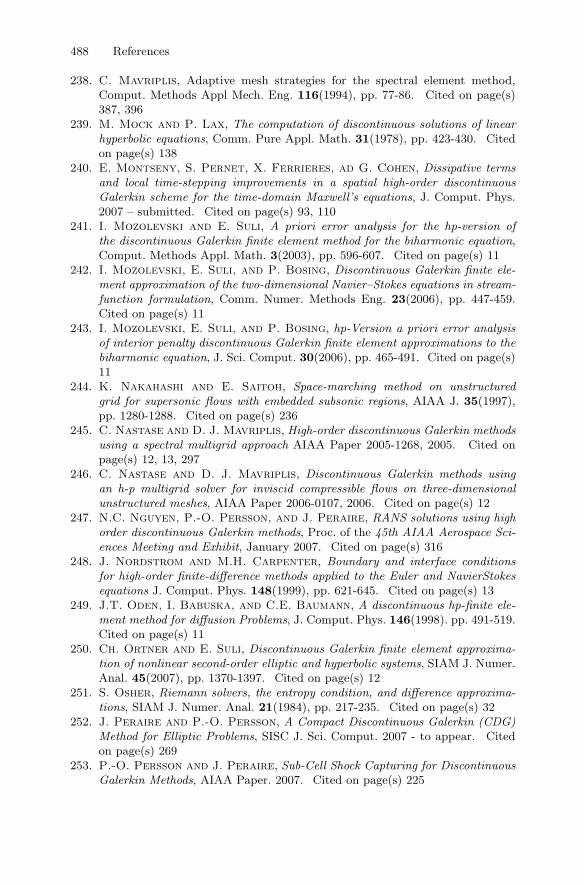
488 References
238. C. Mavriplis, Adaptive mesh strategies for the spectral element method,Comput. Methods Appl Mech. Eng. 116(1994), pp. 77-86. Cited on page(s)387, 396
239. M. Mock and P. Lax, The computation of discontinuous solutions of linearhyperbolic equations, Comm. Pure Appl. Math. 31(1978), pp. 423-430. Citedon page(s) 138
240. E. Montseny, S. Pernet, X. Ferrieres, ad G. Cohen, Dissipative termsand local time-stepping improvements in a spatial high-order discontinuousGalerkin scheme for the time-domain Maxwell’s equations, J. Comput. Phys.2007 – submitted. Cited on page(s) 93, 110
241. I. Mozolevski and E. Suli, A priori error analysis for the hp-version ofthe discontinuous Galerkin finite element method for the biharmonic equation,Comput. Methods Appl. Math. 3(2003), pp. 596-607. Cited on page(s) 11
242. I. Mozolevski, E. Suli, and P. Bosing, Discontinuous Galerkin finite ele-ment approximation of the two-dimensional Navier–Stokes equations in stream-function formulation, Comm. Numer. Methods Eng. 23(2006), pp. 447-459.Cited on page(s) 11
243. I. Mozolevski, E. Suli, and P. Bosing, hp-Version a priori error analysisof interior penalty discontinuous Galerkin finite element approximations to thebiharmonic equation, J. Sci. Comput. 30(2006), pp. 465-491. Cited on page(s)11
244. K. Nakahashi and E. Saitoh, Space-marching method on unstructuredgrid for supersonic flows with embedded subsonic regions, AIAA J. 35(1997),pp. 1280-1288. Cited on page(s) 236
245. C. Nastase and D. J. Mavriplis, High-order discontinuous Galerkin methodsusing a spectral multigrid approach AIAA Paper 2005-1268, 2005. Cited onpage(s) 12, 13, 297
246. C. Nastase and D. J. Mavriplis, Discontinuous Galerkin methods usingan h-p multigrid solver for inviscid compressible flows on three-dimensionalunstructured meshes, AIAA Paper 2006-0107, 2006. Cited on page(s) 12
247. N.C. Nguyen, P.-O. Persson, and J. Peraire, RANS solutions using highorder discontinuous Galerkin methods, Proc. of the 45th AIAA Aerospace Sci-ences Meeting and Exhibit, January 2007. Cited on page(s) 316
248. J. Nordstrom and M.H. Carpenter, Boundary and interface conditionsfor high-order finite-difference methods applied to the Euler and NavierStokesequations J. Comput. Phys. 148(1999), pp. 621-645. Cited on page(s) 13
249. J.T. Oden, I. Babuska, and C.E. Baumann, A discontinuous hp-finite ele-ment method for diffusion Problems, J. Comput. Phys. 146(1998). pp. 491-519.Cited on page(s) 11
250. Ch. Ortner and E. Suli, Discontinuous Galerkin finite element approxima-tion of nonlinear second-order elliptic and hyperbolic systems, SIAM J. Numer.Anal. 45(2007), pp. 1370-1397. Cited on page(s) 12
251. S. Osher, Riemann solvers, the entropy condition, and difference approxima-tions, SIAM J. Numer. Anal. 21(1984), pp. 217-235. Cited on page(s) 32
252. J. Peraire and P.-O. Persson, A Compact Discontinuous Galerkin (CDG)Method for Elliptic Problems, SISC J. Sci. Comput. 2007 - to appear. Citedon page(s) 269
253. P.-O. Persson and J. Peraire, Sub-Cell Shock Capturing for DiscontinuousGalerkin Methods, AIAA Paper. 2007. Cited on page(s) 225
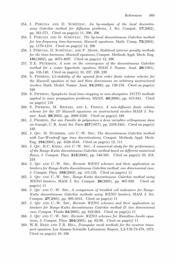
References 489
254. I. Perugia and D. Schotzau, An hp-analysis of the local discontin-uous Galerkin method for diffusion problems, J. Sci. Comput. 17(2002),pp. 561-571. Cited on page(s) 11, 296, 296
255. I. Perugia and D. Schotzau, The hp-local discontinuous Galerkin methodfor low-frequency time-harmonic Maxwell equations, Math. Comp. 72(2003),pp. 1179-1214. Cited on page(s) 12, 296
256. I. Perugia, D. Schotzau, and P. Monk, Stabilized interior penalty methodsfor the time-harmonic Maxwell equations, Comput. Methods Appl. Mech. Eng.191(2002), pp. 4675-4697. Cited on page(s) 12, 296
257. T.E. Peterson, A note on the convergence of the discontinuous Galerkinmethod for a scalar hyperbolic equation, SIAM J. Numer. Anal. 28(1991),pp. 133-140. Cited on page(s) 10, 237, 238, 238
258. S. Piperno, L2-stability of the upwind first order finite volume scheme forthe Maxwell equation in two and three dimensions on arbitrary unstructuredmeshes, Math. Model. Numer. Anal. 34(2000), pp. 139-158. Cited on page(s)348
259. S. Piperno, Symplectic local time-stepping in non-dissipative DGTD methodsapplied to wave propagation problems, M2AN, 40(2006), pp. 815-841. Citedon page(s) 110
260. S. Piperno, M. Remaki, and L. Fezoui, A non-diffusive finite volumescheme for the 3D Maxwell equations on unstructured meshes SIAM J. Nu-mer. Anal. 39(2002), pp. 2089-2108. Cited on page(s) 348
261. J. Proriol, Sur une Famille de polynomes a deux variables orthogonaux dansun triangle, C. R. Acad. Sci. Paris 257(1957), pp. 2459-2461. Cited on page(s)449
262. J. Qiu, M. Dumbser, and C.-W. Shu, The discontinuous Galerkin methodwith Lax-Wendroff type time discretizations, Comput. Methods Appl. Mech.Eng. 194(2005), pp. 4528-4543. Cited on page(s) 12, 111
263. J. Qiu, B.C. Khoo, and C.-W. Shu, A numerical study for the performanceof the Runge-Kutta discontinuous Galerkin method based on different numericalfluxes, J. Comput. Phys. 212(2006), pp. 540-565. Cited on page(s) 33, 218,224
264. J. Qiu and C.-W. Shu, Hermite WENO schemes and their application aslimiters for Runge-Kutta discontinuous Galerkin method: one dimensional case,J. Comput. Phys. 193(2003), pp. 115-135. Cited on page(s) 11
265. J. Qiu and C.-W. Shu, Runge-Kutta discontinuous Galerkin method usingWENO limiters, SIAM J. Sci. Comput. 26(2005), pp. 907-929. Cited onpage(s) 11
266. J. Qiu and C.-W. Shu, A comparison of troubled cell indicators for Runge-Kutta discontinuous Galerkin methods using WENO limiters, SIAM J. Sci.Comput. 27(2005), pp. 995-1013. Cited on page(s) 11
267. J. Qiu and C.-W. Shu, Hermite WENO schemes and their application aslimiters for Runge-Kutta discontinuous Galerkin method II: two dimensionalcase, Comput. Fluids 34(2005), pp. 642-663. Cited on page(s) 11
268. J. Qiu and C.-W. Shu, Hermite WENO schemes for Hamilton-Jacobi equa-tions, J. Comput. Phys. 204(2005), pp. 82-99. Cited on page(s) 11
269. W.H. Reed and T.R. Hill, Triangular mesh methods for the neutron trans-port equation, Los Alamos Scientific Laboratory Report, LA-UR-73-479, 1973.Cited on page(s) 10, 236
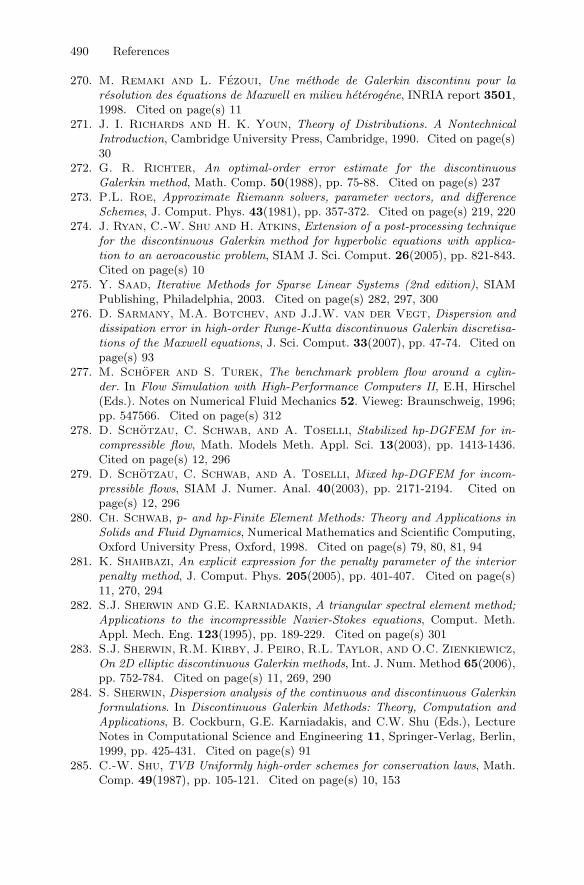
490 References
270. M. Remaki and L. Fezoui, Une methode de Galerkin discontinu pour laresolution des equations de Maxwell en milieu heterogene, INRIA report 3501,1998. Cited on page(s) 11
271. J. I. Richards and H. K. Youn, Theory of Distributions. A NontechnicalIntroduction, Cambridge University Press, Cambridge, 1990. Cited on page(s)30
272. G. R. Richter, An optimal-order error estimate for the discontinuousGalerkin method, Math. Comp. 50(1988), pp. 75-88. Cited on page(s) 237
273. P.L. Roe, Approximate Riemann solvers, parameter vectors, and differenceSchemes, J. Comput. Phys. 43(1981), pp. 357-372. Cited on page(s) 219, 220
274. J. Ryan, C.-W. Shu and H. Atkins, Extension of a post-processing techniquefor the discontinuous Galerkin method for hyperbolic equations with applica-tion to an aeroacoustic problem, SIAM J. Sci. Comput. 26(2005), pp. 821-843.Cited on page(s) 10
275. Y. Saad, Iterative Methods for Sparse Linear Systems (2nd edition), SIAMPublishing, Philadelphia, 2003. Cited on page(s) 282, 297, 300
276. D. Sarmany, M.A. Botchev, and J.J.W. van der Vegt, Dispersion anddissipation error in high-order Runge-Kutta discontinuous Galerkin discretisa-tions of the Maxwell equations, J. Sci. Comput. 33(2007), pp. 47-74. Cited onpage(s) 93
277. M. Schofer and S. Turek, The benchmark problem flow around a cylin-der. In Flow Simulation with High-Performance Computers II, E.H, Hirschel(Eds.). Notes on Numerical Fluid Mechanics 52. Vieweg: Braunschweig, 1996;pp. 547566. Cited on page(s) 312
278. D. Schotzau, C. Schwab, and A. Toselli, Stabilized hp-DGFEM for in-compressible flow, Math. Models Meth. Appl. Sci. 13(2003), pp. 1413-1436.Cited on page(s) 12, 296
279. D. Schotzau, C. Schwab, and A. Toselli, Mixed hp-DGFEM for incom-pressible flows, SIAM J. Numer. Anal. 40(2003), pp. 2171-2194. Cited onpage(s) 12, 296
280. Ch. Schwab, p- and hp-Finite Element Methods: Theory and Applications inSolids and Fluid Dynamics, Numerical Mathematics and Scientific Computing,Oxford University Press, Oxford, 1998. Cited on page(s) 79, 80, 81, 94
281. K. Shahbazi, An explicit expression for the penalty parameter of the interiorpenalty method, J. Comput. Phys. 205(2005), pp. 401-407. Cited on page(s)11, 270, 294
282. S.J. Sherwin and G.E. Karniadakis, A triangular spectral element method;Applications to the incompressible Navier-Stokes equations, Comput. Meth.Appl. Mech. Eng. 123(1995), pp. 189-229. Cited on page(s) 301
283. S.J. Sherwin, R.M. Kirby, J. Peiro, R.L. Taylor, and O.C. Zienkiewicz,On 2D elliptic discontinuous Galerkin methods, Int. J. Num. Method 65(2006),pp. 752-784. Cited on page(s) 11, 269, 290
284. S. Sherwin, Dispersion analysis of the continuous and discontinuous Galerkinformulations. In Discontinuous Galerkin Methods: Theory, Computation andApplications, B. Cockburn, G.E. Karniadakis, and C.W. Shu (Eds.), LectureNotes in Computational Science and Engineering 11, Springer-Verlag, Berlin,1999, pp. 425-431. Cited on page(s) 91
285. C.-W. Shu, TVB Uniformly high-order schemes for conservation laws, Math.Comp. 49(1987), pp. 105-121. Cited on page(s) 10, 153
References 491
286. C.-W. Shu, TVD Time-discretizations, SIAM J. Sci. Stat. Comput. 9(1988),pp. 1073-1084. Cited on page(s) 10, 12
287. C.-W. Shu and P. Wong, A note on the accuracy of spectral method appliedto nonlinear conservation laws, J. Sci. Comput. 10(1995), pp. 357-369. Citedon page(s) 138
288. C.-W. Shu, Different formulations of the discontinuous Galerkin methods fordiffusion problems. In Advances in Scientific Computing, Science Press, Beijing,2001, pp. 144-155. Cited on page(s) 11, 243
289. P. Silvester, Finite element solution of homogeneous waveguide problems,Alta Frequenza 38(1969), pp. 313-317. Cited on page(s) 331
290. J. Smoller, Shock Waves and Reaction-Diffusion Equations, Springer-Verlag,New York, 1983. Cited on page(s) 118
291. A. Solonomoff, A fast algorithm for spectral differentiation, J. Comput.Phys. 98(1992), pp. 174-177. Cited on page(s) 54
292. R. Spiteri and S. Ruuth, A new class of optimal high-order strong stabil-ity preserving time discretization methods, SIAM J. Numer. Anal. 40(2002),pp. 469-491. Cited on page(s) 158
293. G. Strang and G.J. Fix, Analysis of the Finite Element Method Prentice-Hall, Englewood Cliffs, NJ, 1973. Cited on page(s) 6
294. A. H. Stroud, Approximate Calculation of Multiple Integrals, Prentice-Hall,Englewood Cliffs, NJ, 1971. Cited on page(s) 211, 379
295. Y.Z. Sun and Z.J. Wang, Evaluation of discontinuous Galerkin and spectralvolume methods for scalar and system conservation laws on unstructured grids,Int. J. Numer. Meth. Fluids 45(2004), pp. 819-838. Cited on page(s) 13
296. G. Szego, Orthogonal Polynomials, Colloquium Publications 23, AmericanMathematical Society, Providence, RI, 1939. Cited on page(s) 45, 45, 79, 97,445, 445
297. E. Tadmor, The exponential accuracy of Fourier and Chebyshev differencingmethods SIAM J. Numer. Anal. 23(1986), pp. 1-10. Cited on page(s) 79
298. J. Tanner and E. Tadmor, Adaptive mollifiers - high resolution recover ofpiecewise smooth data from its spectral information, Found. Comput. Math.2(2002), pp. 155-189. Cited on page(s) 143
299. A. Taube, M. Dumbser, D.S. Balsara, and C.-D. Munz, Arbitrary high-order discontinuous Galerkin schemes for the magnetohydrodynamic equations,J. Sci Comput. 30(2007), pp. 441-464. Cited on page(s) 12, 112
300. M. Taylor, B. Wingate, and R.E. Vincent, An algorithm for computingFekete points in the triangle, SIAM J. Num. Anal. 38(2000), pp. 1707–1720.Cited on page(s) 175
301. J.W. Thomas, Numerical Partial Differential Equations: Conservation Lawsand Elliptic Equations, Springer Texts in Applied Mathematics 33, Springer-Verlag, New York, 1999. Cited on page(s) 116, 118, 150, 218, 224
302. V.A. Titarev and E.F. Toro, ADER schemes for three-dimensionalnonlinear hyperbolic systems, J. Comput. Phys. 204(2005), pp. 715-736.Cited on page(s) 12, 112
303. E.F. Toro, Riemann Solvers and Numerical Methods for Fluid Dynamics. APractical Introduction (2nd Ed.), Springer-Verlag, New York, 1999. Cited onpage(s) 4, 36, 224
304. E.F. Toro, M. Spruce, and W. Speares, Restoration of the contact surfacein the Harten-Lax-van Leer Riemann Solver, J. Shock Waves 4(1994), pp. 25-34. Cited on page(s) 223, 224
492 References
305. A. Toselli and O. Widlund, Domain Decomposition Methods - Algorithmsand Theory, Springer-Verlag, New York, 2005. Cited on page(s) 282
306. I. Toulopoulos and J.A. Ekaterinaris, High-order discontinuous Galerkindiscretizations for computational aeroacoustics in complex domains, AIAA J.44(2006), pp. 502-511. Cited on page(s) 11
307. L.N. Trefethen, Spectral Methods in Matlab, SIAM Publishing, Philadelphia,2000. Cited on page(s) 29, 49
308. L. N. Trefethen and D. Bau, III, Numerical Linear Algebra, SIAM Pub-lishing, Philadelphia, 1997. Cited on page(s) 297, 300
309. L.N. Trefether and M.R. Trummer, An instability phenomenon in spectralmethods, SIAM J. Numer. Anal. 24(1987) pp. 1008-1023. Cited on page(s) 96
310. S. Tu and S. Aliabadi, A slope limiting procedure in discontinuous Galerkinfinite element method for gasdynamic applications, Int. J. Numer. Anal. Model.2(2005), pp. 163-178. Cited on page(s) 225, 230
311. B. van Leer and S. Nomura, Discontinuous Galerkin for diffusion, AIAApaper 2005-5108. Cited on page(s) 260
312. J.J. W. van der Vegt and H. van der Ven, Space-time discontinuousGalerkin finite element method with dynamic grid motion for inviscid compress-ible flows. I. General formulation, J. Comput. Phys. 182(2002), pp. 546-585.Cited on page(s) 112
313. H. Vandeven, Family of spectral filters for discontinuous problems, J. Sci.Comput. 8(1991), pp. 159-192. Cited on page(s) 143
314. J.L. Volakis, A. Chatterjee, and L. Kempel, Finite Element Methods forElectromagnetics: Antennas, Microwave Circuits and Scattering Applications,IEEE Press, New York, 1998. Cited on page(s) 332
315. S. Wandzura and H. Xiao, Symmetric quadrature rules on a triangle, Com-put. Math. Applica. 45(2003), pp. 1829-1840. Cited on page(s) 379
316. Z.J. Wang, Spectral (finite) volume method for conservation laws on unstruc-tured grids: Basic formulation, J. Comput. Phys. 178(2002), pp. 210-251.Cited on page(s) 13
317. Z.J. Wang and Y. Liu, Spectral (finite) volume method for conservation lawson unstructured grids II: Extension to two-dimensional scalar equation, J. Com-put. Phys. 179(2002), pp. 665-697. Cited on page(s) 13
318. T. Warburton, Application of the discontinuous Galerkin method toMaxwell’s equations using unstructured polymorphic hp-finite elements. InDiscontinuous Galerkin Methods: Theory, Computation and Applications, B.Cockburn, G.E. Karniadakis, and C.W. Shu (Eds), Lecture Notes in Computa-tional Science and Engineering 11, Springer-Verlag, Berlin, 1999, pp. 451-458.Cited on page(s) 11, 348
319. T. Warburton and M. Embree, The role of the penalty in the local discon-tinuous Galerkin method for Maxwell’s eigenvalue problem, Comput. MethodsAppl. Mech. Eng. 195(2006), pp. 3205-3223. Cited on page(s) 12, 341
320. T. Warburton and J.S. Hesthaven, On the constants in hp-finite elementtrace inverse inequalities, Comput. Methods Appl. Mech. Eng. 192(2003),pp. 2765-2773. Cited on page(s) 94, 292
321. T. Warburton and T. Hagstrom, Taming the CFL number for discontinu-ous Galerkin methods on structured meshes, J. Comput. Phys. 2006 – submit-ted. Cited on page(s) 105, 105
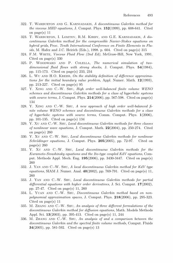
References 493
322. T. Warburton and G. Karniadakis, A discontinuous Galerkin method forthe viscous MHD equations, J. Comput. Phys. 152(1999), pp. 608-641. Citedon page(s) 11
323. T. Warburton, I. Lomtev, R.M. Kirby, and G.E. Karniadakis, A dis-continuous Galerkin method for the compressible Navier-Stokes equations onhybrid grids, Proc. Tenth International Conference on Finite Elements in Flu-ids, M. Hafez and J.C. Heirich (Eds.), 1998. p. 604. Cited on page(s) 315
324. F.M. White, Viscous Fluid Flow (2nd Ed), McGraw-Hill, New York, 1991.Cited on page(s) 330
325. P. Woodward and P. Colella, The numerical simulation of two-dimensional fluid flows with strong shocks, J. Comput. Phys. 54(1984),pp. 115-173. Cited on page(s) 233, 234
326. L. Wu and H.O. Kreiss, On the stability definition of difference approxima-tions for the initial boundary value problem, Appl. Numer. Math. 12(1993),pp. 213-227. Cited on page(s) 95
327. Y. Xing and C.-W. Shu, High order well-balanced finite volume WENOschemes and discontinuous Galerkin methods for a class of hyperbolic systemswith source terms, J. Comput. Phys. 214(2006), pp. 567-598. Cited on page(s)134
328. Y. Xing and C.-W. Shu, A new approach of high order well-balanced fi-nite volume WENO schemes and discontinuous Galerkin methods for a classof hyperbolic systems with source terms, Comm. Comput. Phys. 1(2006),pp. 101-135. Cited on page(s) 134
329. Y. Xu and C.-W. Shu, Local discontinuous Galerkin methods for three classesof nonlinear wave equations, J. Comput. Math. 22(2004), pp. 250-274. Citedon page(s) 260
330. Y. Xu and C.-W. Shu, Local discontinuous Galerkin methods for nonlinearSchrodinger equations, J. Comput. Phys. 205(2005), pp. 72-97. Cited onpage(s) 260
331. Y. Xu and C.-W. Shu, Local discontinuous Galerkin methods for theKuramoto-Sivashinsky equations and the Ito-type coupled KdV equations, Com-put. Methods Appl. Mech. Eng. 195(2006), pp. 3430-3447. Cited on page(s)260
332. J. Yan and C.-W. Shu, A local discontinuous Galerkin method for KdV typeequations, SIAM J. Numer. Anal. 40(2002), pp. 769-791. Cited on page(s) 11,260
333. J. Yan and C.-W. Shu, Local discontinuous Galerkin methods for partialdifferential equations with higher order derivatives, J. Sci. Comput. 17(2002),pp. 27-47. Cited on page(s) 11, 260
334. L. Yuan and C.-W. Shu, Discontinuous Galerkin method based on non-polynomial approximation spaces, J. Comput. Phys. 218(2006), pp. 295-323.Cited on page(s) 11
335. M. Zhang and C.-W. Shu, An analysis of three different formulations of thediscontinuous Galerkin method for diffusion equations, Math. Models MethodsAppl. Sci. 13(2003), pp. 395-413. Cited on page(s) 11, 244
336. M. Zhang and C.-W. Shu, An analysis of and a comparison between thediscontinuous Galerkin and the spectral finite volume methods, Comput. Fluids34(2005), pp. 581-592. Cited on page(s) 13
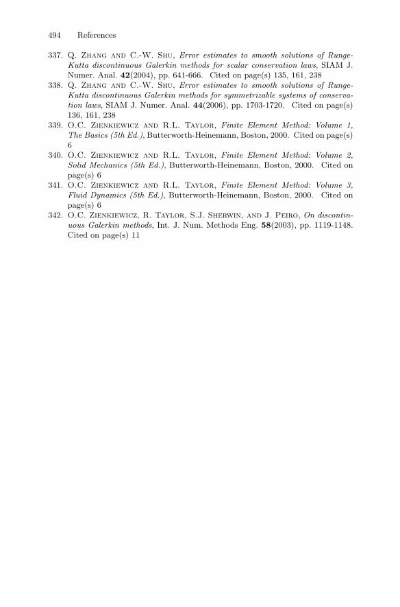
494 References
337. Q. Zhang and C.-W. Shu, Error estimates to smooth solutions of Runge-Kutta discontinuous Galerkin methods for scalar conservation laws, SIAM J.Numer. Anal. 42(2004), pp. 641-666. Cited on page(s) 135, 161, 238
338. Q. Zhang and C.-W. Shu, Error estimates to smooth solutions of Runge-Kutta discontinuous Galerkin methods for symmetrizable systems of conserva-tion laws, SIAM J. Numer. Anal. 44(2006), pp. 1703-1720. Cited on page(s)136, 161, 238
339. O.C. Zienkiewicz and R.L. Taylor, Finite Element Method: Volume 1,The Basics (5th Ed.), Butterworth-Heinemann, Boston, 2000. Cited on page(s)6
340. O.C. Zienkiewicz and R.L. Taylor, Finite Element Method: Volume 2,Solid Mechanics (5th Ed.), Butterworth-Heinemann, Boston, 2000. Cited onpage(s) 6
341. O.C. Zienkiewicz and R.L. Taylor, Finite Element Method: Volume 3,Fluid Dynamics (5th Ed.), Butterworth-Heinemann, Boston, 2000. Cited onpage(s) 6
342. O.C. Zienkiewicz, R. Taylor, S.J. Sherwin, and J. Peiro, On discontin-uous Galerkin methods, Int. J. Num. Methods Eng. 58(2003), pp. 1119-1148.Cited on page(s) 11
Index
Adams-Bashforth method, 301Adaptivity, 386, 396ADER-DG, 110, 112Adjoint problem, 137, 291Affine mapping, 44, 171, 172, 410Aliasing, 81, 125, 211, 254
instability, 125, 127, 211stabilization, 127
Barycentric coordinates, 171, 409Basis function, 5
orthonormal, 78three-dimensional, 411, 449two-dimensional, 173, 449
BCType matrix, 199, 451, 457, 458Blending function, 177, 413Boundary conditions
Dirichlet, 25, 26, 248, 274inhomogeneous, 249, 273Neumann, 249, 275
Boundeduniform, 145
Burgers’ equation, 117, 141, 143, 154,159
viscous, 255
CFL condition, 66, 97, 98Coercivity, 287, 292
central flux, 294internal penalty flux, 294LDG flux, 294
Condition number, 44, 269, 271Conservation
global, 120local, 119
Conservation lawconservation, 119convergence of DG-FEM, 161convex flux, 117multidimensional, 34nonconvex flux, 118scalar, 1, 31, 115, 120strong DG-FEM form, 119system, 33three dimensions, 407two dimensions, 169weak DG-FEM form, 119
Consistency, 77, 291adjoint, 292
Continuity, 294Convection-diffusion equation, 255Convergence, 76Cubature, 212, 379
implementation, 212Curvilinear element, 212, 213, 373
mapping, 375operators, 378
DG average ·, 20, 288DG jump [[·]], 20, 288Differentiation matrix, 52, 184, 185,
419, 420Discontinuous Galerkin finite element
method (DG-FEM), 7, 23Dispersion analysis, 88
central flux, 92resolution, 92upwind flux, 91
496 Index
Dispersion relationcentral flux, 90exact, 88, 89numerical, 89upwind flux, 90
Dispersive equation, 257, 259DistMesh, 453Divergence free basis, 356
E-flux, 32, 122Elliptic problem, 261Energy method, 24, 25, 84, 247Entropy
condition, 117convex, 117, 121discrete cell condition, 122flux, 117, 121Lax condition, 118
Equivalence theorem, 77Error equation, 76, 86Error estimate
heat equationcentral flux, 251LDG flux, 253
Laplace eigenvalues, 337Laplace eigenvectors, 338linear hyperbolic problem, 85, 88, 236multidimensional, 236nonlinear conservation law, 135, 238nonlinear conservation laws, 160Poisson equation, 296
Error estimationa posteriori methods, 386adjoint method, 386smoothness indicator, 387superconvergence, 386
EToE matrix, 59, 193, 427, 457EToF matrix, 59, 193, 428EToV matrix, 56, 190, 451Euler equations
conservation form, 207Couette flow, 216, 233forward facing step, 233isentropic vortex, 209one-dimensional, 161scramjet inlet flow, 234Sod’s problem, 165two-dimensional, 206
FactorizationCholesky, 215, 298LU, 297
Filter, 211exponential, 129, 139function, 129, 130matrix, 130, 186Pade based, 143parameter choice, 132physical space, 143
Finite difference method (FDM), 1Finite element method (FEM), 6Finite volume method (FVM), 3, 32Flux-Jacobian, 169FToF matrix, 58, 192FToV matrix, 58, 192
Galerkin orthogonality, 86Galerkin scheme, 5, 23Geometry conforming grid, 72Gibbs phenomenon, 137
Hamilton-Jacobi equation, 134, 135Heat equation, 243, 245, 260Helmholtz equation, 280, 307, 342High-order problems, 245Higher-order equation, 257, 260History of DG-FEM, 10
Interpolation, 81Iterative methods, 299
Jacobian, 57, 172, 191, 379, 410, 426
Lagrange polynomialone dimension, 5, 47three dimensions, 409two dimensions, 171
Laplace equationeigenvalue problem, 334, 335interor penalty, 337
Lebesque constant, 47, 49, 178, 414Lifting operator, 289, 290Limiter, 145, 148
generalized slope limiter, 152gradient limiter, 225hierarchic modal slope limiter, 156MUSCL, 150slope limiter, 148, 152, 224two dimensions, 224
Linear hyperbolic system, 37
Index 497
Mapping metric, 57Mass matrix
edge, 187, 421global, 6local, 9, 23, 24, 52, 183, 418
Matlab scriptAdvec1D.m, 66AdvecDriver1D.m, 67AdvecRHS1D.m, 65BuildBCMaps2D.m, 200BuildCurvedOPS2D.m, 380BuildHNonCon2D.m, 390BuildMaps1D.m, 60BuildMaps2D.m, 194BuildMaps3D.m, 428BuildPNonCon2D.m, 398BurgersRHS1D.m, 255Connect1D.m, 59Connect2D.m, 193ConstructMap.m, 459CorrectBCTable.m, 458Cubature2D.m, 212Curl2D.m, 190Curl3D.m, 424CurvedCNSRHS2D.m, 320CurvedDGDiv2D.m, 318CurvedDGGrad2D.m, 316CurvedDGJump2D.m, 319CurvedEulerRHS2D.m, 213, 214CurvedINS2D.m, 305, 307CurvedINSViscous2D.m, 307CurvedPoissonIPDG2D.m, 283CurvedPoissonIPDGDriver2D.m, 286DispersiveLDGRHS1D.m, 258Div2D.m, 189Div3D.m, 423Dmatrices2D.m, 185Dmatrices3D.m, 420Dmatrix1D.m, 53dtscale2D.m, 199Euler1D.m, 163EulerDriver1D.m, 163EulerFluxes2D.m, 207EulerHLL2D.m, 223EulerLF2D.m, 214EulerLimiter2D.m, 226EulerRHS1D.m, 162EulerRHS2D.m, 208EulerRoe2D.m, 220
evalshift.m, 412Filter1D.m, 130Filter2D.m, 186GeometricFactors1D.m, 57GeometricFactors2D.m, 191GeometricFactors3D.m, 425Globals1D.m, 62Globals2D.m, 195Globals3D.m, 430Grad2D.m, 189Grad3D.m, 423GradJacobiP.m, 52GradSimplex2DP.m, 184GradSimplex3DP.m, 419GradVandermonde1D.m, 52GradVandermonde2D.m, 184GradVandermonde3D.m, 420Heat1D.m, 249HeatCRHS1D.m, 248HeatCstabRHS1D.m, 263HeatDriver1D.m, 250HeatLDGRHS1D.m, 252Hrefine2D.m, 388INSAdvection2D.m, 303INSLiftDrag2D.m, 313INSPressure2D.m, 305JacobiGL.m, 47, 448JacobiGQ.m, 46, 447JacobiP.m, 45, 446Lift1D.m, 56Lift2D.m, 188Lift3D.m, 422MakeCylinder2D.m, 376Maxwell1D.m, 70Maxwell2D.m, 203MaxwellCurvedRHS2D.m, 384MaxwellDriver1D.m, 70MaxwellDriver2D.m, 204MaxwellHNonConRHS2D.m, 394MaxwellPNonConRHS2D.m, 403MaxwellRHS1D.m, 68MaxwellRHS2D.m, 202MaxwellRHS3D.m, 435MeshGen1D.m, 451MeshGenDistMesh1D.m, 455MeshGenDistMesh2D.m, 456MeshReaderGambit1D.m, 452minmod.m, 150minmodB.m, 153
498 Index
Nodes2D.m, 179Nodes3D.m, 414Normals1D.m, 57Normals2D.m, 191Normals3D.m, 426PlotAdaptiveContour2D.m, 467PlotAdaptiveContour3D.m, 469PlotContour2D.m, 466PlotContour3D.m, 468PlotDomain2D.m, 465PlotField2D.m, 465PlotMesh2D.m, 465PlotSlice3D.m, 470Poisson2D.m, 276PoissonCDriver1D.m, 267PoissonCstab1D.m, 266PoissonCstabRHS1D.m, 265PoissonDriver2D.m, 277PoissonIPDG2D.m, 278PoissonIPDG3D.m, 438PoissonIPstabRHS1D.m, 270PoissonRHS2D.m, 275rstoab.m, 173rsttoabc.m, 411Simplex2DP.m, 173, 449Simplex3DP.m, 411, 450SlopeLimit1.m, 151SlopeLimitLin.m, 150SlopeLimitN.m, 152SpectralCNSDriver2D.m, 327StartUp1D.m, 61StartUp2D.m, 195StartUp3D.m, 430tiConnect3D.m, 428Vandermonde1D.m, 50Vandermonde2D.m, 183Vandermonde3D.m, 417Warpfactor.m, 177WarpShiftFace3D.m, 412xytors.m, 181xyztorst.m, 416
Maxwell’s equationscavity solution, 71, 205, 436curl-curl form, 331, 342
stabilized, 369curvilinear elements, 383eigenvalues, 342frequency domain, 342general flux, 348
nonconforming elements, 394numerical flux, 68, 202, 433one dimension, 38, 67Sobolev spaces, 349spurious modes, 331
central flux, 344upwind flux, 344, 370
stabilized, 371three dimensions, 342, 432
eigenvalues, 367two dimensions, 200
eigenvalues, 346, 348, 364Metric, 172, 410Minmod function, 149
variation bounded, 153Modal form, 20, 22, 44
Navier-Stokes equationscompressible, 314, 319
pressure pulse, 326shear flow, 326stress tensor, 320
incompressible, 300benchmarks, 308drag, 313Kovasznay flow, 308lift, 313Vortex flow, 310
Nodal form, 21, 23, 46, 50, 181Nodes
tetrahedron, 412triangle, 174
Nonconforming discretizations, 386element refinement, 388intersection test, 391nonconforming elements
Maxwell’s equations, 394operators, 390refinement, 387
nonconforming order, 396Maxwell’s equations, 400
Nonconservative form, 134Norm
broken, 19, 75discontinuous Galerkin, 292global, 19local, 19semi, 76
Index 499
Sobolev, 75total variation, 146
Normal vector, 191, 426Notation, 19, 75Numerical flux, 8, 22, 24, 32, 217, 246
approximate Riemann solver, 218central, 26, 65, 84, 86, 205, 246, 258consistent, 32dispersive equation, 258E-flux, 32, 122exact Riemann solver, 218flux splitting, 136heat equation, 246HLL, 222HLLC, 224internal penalty, 269, 275, 290, 337Lax-Friedrichs, 32, 34, 119, 303
global, 32local, 33, 170, 208, 408
linear scalar problem, 25, 26linear system, 34llinear Roe, 222local discontinuous Galerkin (LDG),
252, 258, 267Maxwell’s equations, 348monotone, 32penalty term, 263Roe condition, 219Roe linearization, 219stabilized, 263, 267, 335upwind, 26, 35, 65, 84, 205
Penalty parameter, 270, 293, 335, 369central flux, 271internal penalty, 294internal penalty flux, 272LDG flux, 272Maxwell’s equations, 348spectral impact, 338, 340
Phase error, 92Poisson equation, 261, 266, 287, 297,
305spectrum, 334three dimensions, 437two-dimensional, 275
Polynomialcanonical basis, 44, 173, 411Gegenbauer, 145Jacobi, 45, 445
Legendre, 45, 47, 49, 78, 445orthonormal three-dimensional, 411orthonormal two-dimensional, 173symmetric Jacobi, 49
Preconditioner, 281, 299block-Jacobi, 282incomplete Cholesky, 282, 299incomplete LU, 282Jacobi, 282
Pressure projection, 302Projection, 44, 78
Quadrature, 447Gauss, 46, 447Gauss-Lobatto, 47, 49Gauss-Radau, 88
Rankine-Hugoniot condition, 36, 117,218
Recurrence, 45, 445Reexpansion
Gegenbauer, 145Pade, 143
Reference element, 44, 171, 409Residual, 2, 7, 21Reverse Cuthill-McKee bandwidth
minimization, 298Riemann problem, 36, 218
linearized, 219Roe linearization, 219
Runge phenomenon, 49Runge-Kutta method, 157
explicit, 63, 93, 101linear problem, 101low storage, 64strong stability preserving (SSP-RK),
158total variation diminishing (TVD-
RK), 158
Semidiscrete scheme, 76, 119Shock, 116Simultaneous approximation term
(SAT) schemes, 13Space-time DG-FEM, 112Sparsity, 268Spectral method, 79Spectral penalty method, 13, 24Spectral properties, 331
500 Index
Maxwell’s equations, 367divergence free basis, 356polynomial basis, 350
penalty parameter, 338spurious modes, 331, 333, 337, 344,
368Stability, 77, 83
central flux, 294dispersive equation, 258heat equation, 247, 251internal penalty flux, 294LDG flux, 294linear system, 84linear wave equation, 25nonlinear, 121, 122
Stability region, 93Stiffly stable timeintegration, 301Stiffness matrix
global, 6local, 9, 23, 24, 52, 53, 185, 246, 420
Strong DG-FEM form, 8, 9, 22, 23, 34,119, 170, 246, 408
Sturm-Liouville problem, 78, 129Surface integral, 55, 187, 188, 421, 422Symmetry, 264, 290
Test function, 5, 21Timestep
compressible Navier-Stokes equations,325
heat equation, 250hyperbolic system, 97local, 108three dimensions, 432
two dimensions, 199wave equation, 97, 197
Total variationbounded in the mean (TVBM), 153diminishing in the mean (TVDM),
148norm, 146
Trace inequality, 87, 94, 292Truncation error, 76
Vandermonde matrix, 46, 50, 173, 182,410, 417
Variational crime, 210Vertex
coordinates, 56, 190, 425, 451map mapI , 457map mapO, 457map vmapB, 194, 199, 428map vmapI , 200map vmapM , 60, 194, 228, 428map vmapO, 200map vmapP , 60, 194, 228, 428renumbering, 389
Viscosity solution, 117
Warp function, 175, 178, 412, 414Wave equation, 20, 64, 148, 153Weak curl operator
Dirichlet boundary conditions, 343Neumann boundary conditions, 343
Weak DG-FEM form, 8, 9, 22, 23, 31,34, 119, 170, 246, 408
Weak solution, 116, 120, 133Well-posedness, 76
Texts in Applied Mathematics(continued from page ii)
28. Gustafson/Wilcox: Analytical and Computational Methods of AdvancedEngineering Mathematics (1998).
29. Tveito/Winther: Introduction to Partial Differential Equations:A Computational Approach (1998).
30. Gasquet/Witomski: Fourier Analysis and Applications: Filtering,Numerical Computation, Wavelets (1998).
31. Bremaud: Markov Chains: Gibbs Fields, Monte Carlo Simulation,and Queues (1999).
32. Durran: Numerical Methods for Wave Equations in Geophysical FluidDynamics (1998).
33. Thomas: Numerical Partial Differential Equations: ConservationLaws and Elliptic Equations (1999).
34. Chicone: Ordinary Differential Equations with Applications (1999)(second edition, 2005).
35. Kevorkian: Partial Differential Equations: Analytical SolutionTechniques, 2nd ed. (1999).
36. Dullerud/Paganini: A Course in Robust Control Theory:A Convex Approach (2000).
37. Quarteroni/Sacco/Saleri: Numerical Mathematics (2000).38. Gallier: Geometric Methods and Applications: For Computer Science
and Engineering (2000).39. Atkinson/Han: Theoretical Numerical Analysis: A Functional Analysis
Framework (2001) (second edition, 2005).40. Brauer/Castillo-Chavez: Mathematical Models in Population Biology
and Epidemiology (2001).41. Davies: Integral Transforms and Their Applications, 3rd ed. (2002).42. Deuflhard/Bornemann: Scientific Computing with Ordinary
Differential Equations (2002).43. Deuflhard/Hohmann: Numerical Analysis in Modern Scientific
Computing: An Introduction, 2nd ed. (2003).44. Knabner/Angerman: Numerical Methods for Elliptic and Parabolic Partial
Differential Equations (2003).45. Larsson/Thomee: Partial Differential Equations
with Numerical Methods (2003).46. Pedregal: Introduction to Optimization (2003).47. Ockendon/Ockendon: Waves and Compressible Flow (2004).48. Hinrichsen/Pritchard: Mathematical Systems Theory I (2004).49. Bullo: Geometric Control of Mechanical Systems (2004).50. Verhulst: Methods and Applications of Singular Perturbations (2005).
(second edition, 2007).51. Bondeson: Computational Electromagnetics (2005).52. Holmes: Introduction to Numerical Methods in Differential Equations (2006).53. Stuart/Pavliotis: Multiscale Methods: Averaging and Homogenization (2007).54.55. Allaire/Kaber: Numerical Linear Algebra (2007).
Hesthaven/Warburton: Nodal Discontinuous Galerkin Methods (2008).


![ON THE DENSENESS OF JACOBI POLYNOMIALS · 2019. 8. 1. · ON THE DENSENESS OF JACOBI POLYNOMIALS 1457 has also been solved in [18]. The best possible cases of general order khave](https://static.fdocument.org/doc/165x107/60e87109eca03f6bf25acc4f/on-the-denseness-of-jacobi-polynomials-2019-8-1-on-the-denseness-of-jacobi.jpg)