
9.QuantumChromodynamics - pdg.lbl.govpdg.lbl.gov/2018/reviews/rpp2018-rev-qcd.pdf ·...
52
9. Quantum chromodynamics 1 9. Quantum Chromodynamics Revised September 2017 by S. Bethke (Max-Planck-Institute of Physics, Munich), G. Dissertori (ETH Zurich), and G.P. Salam (CERN). 1 This update retains the 2016 summary of α s values, as few new results were available at the deadline for this Review. Those and further new results will be included in the next update. 9.1. Basics Quantum Chromodynamics (QCD), the gauge field theory that describes the strong interactions of colored quarks and gluons, is the SU(3) component of the SU(3)×SU(2)×U(1) Standard Model of Particle Physics. The Lagrangian of QCD is given by L = q ¯ ψ q,a (iγ μ ∂ μ δ ab − g s γ μ t C ab A C μ − m q δ ab )ψ q,b − 1 4 F A μν F A μν , (9.1) where repeated indices are summed over. The γ μ are the Dirac γ -matrices. The ψ q,a are quark-field spinors for a quark of flavor q and mass m q , with a color-index a that runs from a = 1 to N c = 3, i.e. quarks come in three “colors.” Quarks are said to be in the fundamental representation of the SU(3) color group. The A C μ correspond to the gluon fields, with C running from 1 to N 2 c − 1 = 8, i.e. there are eight kinds of gluon. Gluons transform under the adjoint representation of the SU(3) color group. The t C ab correspond to eight 3 × 3 matrices and are the generators of the SU(3) group (cf. the section on “SU(3) isoscalar factors and representation matrices” in this Review, with t C ab ≡ λ C ab /2). They encode the fact that a gluon’s interaction with a quark rotates the quark’s color in SU(3) space. The quantity g s is the QCD coupling constant. Finally, the field tensor F A μν is given by F A μν = ∂ μ A A ν − ∂ ν A A μ − g s f ABC A B μ A C ν [t A ,t B ]= if ABC t C , (9.2) where the f ABC are the structure constants of the SU(3) group. Neither quarks nor gluons are observed as free particles. Hadrons are color-singlet (i.e. color-neutral) combinations of quarks, anti-quarks, and gluons. Ab-initio predictive methods for QCD include lattice gauge theory and perturbative expansions in the coupling. The Feynman rules of QCD involve a quark-antiquark- gluon (q ¯ qg ) vertex, a 3-gluon vertex (both proportional to g s ), and a 4-gluon vertex (proportional to g 2 s ). A full set of Feynman rules is to be found for example in Ref. 1. Useful color-algebra relations include: t A ab t A bc = C F δ ac , where C F ≡ (N 2 c − 1)/(2N c )= 4/3 is the color-factor (“Casimir”) associated with gluon emission from a quark; 1 On leave from LPTHE, UMR 7589, CNRS, Paris, France M. Tanabashi et al. (Particle Data Group), Phys. Rev. D 98, 030001 (2018) June 5, 2018 19:47
Transcript of 9.QuantumChromodynamics - pdg.lbl.govpdg.lbl.gov/2018/reviews/rpp2018-rev-qcd.pdf ·...
9. Quantum chromodynamics 1
9. Quantum Chromodynamics
Revised September 2017 by S. Bethke (Max-Planck-Institute of Physics, Munich),G. Dissertori (ETH Zurich), and G.P. Salam (CERN).1
This update retains the 2016 summary of αs values, as few new results were availableat the deadline for this Review. Those and further new results will be included in thenext update.
9.1. Basics
Quantum Chromodynamics (QCD), the gauge field theory that describes thestrong interactions of colored quarks and gluons, is the SU(3) component of theSU(3)×SU(2)×U(1) Standard Model of Particle Physics.
The Lagrangian of QCD is given by
L =∑
q
ψq,a(iγµ∂µδab − gsγµtCabAC
µ − mqδab)ψq,b −1
4FA
µνFA µν , (9.1)
where repeated indices are summed over. The γµ are the Dirac γ-matrices. The ψq,a arequark-field spinors for a quark of flavor q and mass mq, with a color-index a that runsfrom a = 1 to Nc = 3, i.e. quarks come in three “colors.” Quarks are said to be in thefundamental representation of the SU(3) color group.
The ACµ correspond to the gluon fields, with C running from 1 to N2
c − 1 = 8, i.e.
there are eight kinds of gluon. Gluons transform under the adjoint representation of theSU(3) color group. The tCab correspond to eight 3 × 3 matrices and are the generators ofthe SU(3) group (cf. the section on “SU(3) isoscalar factors and representation matrices”in this Review, with tCab ≡ λC
ab/2). They encode the fact that a gluon’s interaction witha quark rotates the quark’s color in SU(3) space. The quantity gs is the QCD couplingconstant. Finally, the field tensor FA
µν is given by
FAµν = ∂µAA
ν − ∂νAAµ − gs fABCAB
µ ACν [tA, tB] = ifABCtC , (9.2)
where the fABC are the structure constants of the SU(3) group.
Neither quarks nor gluons are observed as free particles. Hadrons are color-singlet (i.e.color-neutral) combinations of quarks, anti-quarks, and gluons.
Ab-initio predictive methods for QCD include lattice gauge theory and perturbativeexpansions in the coupling. The Feynman rules of QCD involve a quark-antiquark-gluon (qqg) vertex, a 3-gluon vertex (both proportional to gs), and a 4-gluon vertex(proportional to g2
s). A full set of Feynman rules is to be found for example in Ref. 1.
Useful color-algebra relations include: tAabtAbc = CF δac, where CF ≡ (N2
c − 1)/(2Nc) =4/3 is the color-factor (“Casimir”) associated with gluon emission from a quark;
1 On leave from LPTHE, UMR 7589, CNRS, Paris, France
M. Tanabashi et al. (Particle Data Group), Phys. Rev. D 98, 030001 (2018)June 5, 2018 19:47
2 9. Quantum chromodynamics
fACDfBCD = CAδAB where CA ≡ Nc = 3 is the color-factor associated with gluonemission from a gluon; tAabt
Bab = TRδAB , where TR = 1/2 is the color-factor for a gluon to
split to a qq pair.
The fundamental parameters of QCD are the coupling gs (or αs =g2s
4π) and the quark
masses mq.
There is freedom for an additional CP-violating term to be present in the QCD
Lagrangian, θαs
8πFA
µν FA µν , where FA µν is the dual of the gluon field tensor,1
2ǫµνσρFA σρ,
where ǫµνσρ is the fully antisymmetric Levi-Cevita symbol. Experimental limits on theneutron electric dipole moment [2] constrain the coefficient of this contribution to satisfy|θ| . 10−10. Further discussion is to be found in Ref. 3 and in the Axions section in theListings of this Review.
This section will concentrate mainly on perturbative aspects of QCD as they relateto collider physics. Related textbooks and reviews include Refs. 1,4–8. Aspects specificto Monte Carlo event generators are reviewed in the dedicated section 41. Lattice QCDis also reviewed in a section of its own, Sec. 17, with further discussion of perturbativeand non-perturbative aspects to be found in the sections on “Quark Masses”, “TheCKM quark-mixing matrix”, “Structure Functions”, “Fragmentation Functions”, and“Heavy-Quark and Soft-Collinear Effective Theory” in this Review. For an overviewof some of the QCD issues and recent results in heavy-ion physics, see for exampleRefs. [9–11].
9.1.1. Running coupling :
In the framework of perturbative QCD (pQCD), predictions for observables areexpressed in terms of the renormalized coupling αs(µ
2R), a function of an (unphysical)
renormalization scale µR. When one takes µR close to the scale of the momentumtransfer Q in a given process, then αs(µ
2R ≃ Q2) is indicative of the effective strength of
the strong interaction in that process.
The coupling satisfies the following renormalization group equation (RGE):
µ2R
dαs
dµ2R
= β(αs) = −(b0α2s + b1α
3s + b2α
4s + · · ·) (9.3)
where b0 = (11CA − 4nfTR)/(12π) = (33 − 2nf )/(12π) is referred to as the 1-loop β-
function coefficient, the 2-loop coefficient is b1 = (17C2A − nfTR(10CA + 6CF ))/(24π2) =
(153 − 19nf )/(24π2), and the 3-loop coefficient is b2 = (2857 − 50339 nf + 325
27 n2f )/(128π3)
for the SU(3) values of CA and CF . The 4-loop coefficient, b3, is to be found in Refs. 12,13, while the 5-loop coefficient, b4, is in Refs. 14–16. The coefficients b2 and b3 (andbeyond) are renormalization-scheme-dependent, and given here in the modified minimalsubtraction (MS) scheme [17], by far the most widely used scheme in QCD.
The minus sign in Eq. (9.3) is the origin of Asymptotic Freedom [18,19], i.e. the factthat the strong coupling becomes weak for processes involving large momentum transfers(“hard processes”). For momentum transfers in the 100 GeV – TeV range, αs ∼ 0.1,while the theory is strongly interacting for scales around and below 1 GeV.
June 5, 2018 19:47
9. Quantum chromodynamics 3
The β-function coefficients, the bi, are given for the coupling of an effective theory inwhich nf of the quark flavors are considered light (mq ≪ µR), and in which the remainingheavier quark flavors decouple from the theory. One may relate the coupling for thetheory with nf + 1 light flavors to that with nf flavors through an equation of the form
α(nf +1)s (µ2
R) = α(nf )s (µ2
R)
(
1 +∞∑
n=1
n∑
ℓ=0
cnℓ [α(nf )s (µ2
R)]n lnℓ µ2R
m2h
)
, (9.4)
where mh is the mass of the (nf +1)th flavor, and the first few cnℓ coefficients are
c11 = 16π , c10 = 0, c22 = c211, c21 = 19
24π2 , and c20 = − 1172π2 when mh is the MS mass at
scale mh (c20 = 724π2 when mh is the pole mass — mass definitions are discussed below
and in the review on “Quark Masses”). Terms up to c4ℓ are to be found in Refs. 20, 21.Numerically, when one chooses µR = mh, the matching is a modest effect, owing to thezero value for the c10 coefficient. Relations between nf and (nf +2) flavors where the twoheavy flavors are close in mass are given to three loops in Ref. 22.
Working in an energy range where the number of flavors is taken constant, a simpleexact analytic solution exists for Eq. (9.3) only if one neglects all but the b0 term, givingαs(µ
2R) = (b0 ln(µ2
R/Λ2))−1. Here Λ is a constant of integration, which corresponds to thescale where the perturbatively-defined coupling would diverge. Its value is indicative ofthe energy range where non-perturbative dynamics dominates. A convenient approximateanalytic solution to the RGE that includes the terms up to b4 is given by the iterativesolution of Eq. (9.3)
αs(µ2R) ≃ 1
b0t
(
1 − b1
b20
ℓ
t+
b21(ℓ2 − ℓ − 1) + b0b2
b40t2
+
+b31
(
−2ℓ3 + 5ℓ2 + 4ℓ − 1)
− 6b0b2b1ℓ + b20b3
2b60t3
+
+18b0b2b
21
(
2ℓ2−ℓ−1)
+b41(
6ℓ4−26ℓ3−9ℓ2+24ℓ+7)
6b80t4
+−b20b3b1(12ℓ+1)+2b20
(
5b22+b0b4)
6b80t4
)
, (9.5)
with t ≡ lnµ2
R
Λ2and ℓ = ln t, again parametrized in terms of a constant Λ. Note that
Eq. (9.5) is one of several possible approximate 4-loop solutions for αs(µ2R), and that a
value for Λ only defines αs(µ2R) once one knows which particular approximation is being
used. An alternative to the use of formulas such as Eq. (9.5) is to solve the RGE exactly,numerically (including the discontinuities, Eq. (9.4), at flavor thresholds). In such casesthe quantity Λ does directly arise (though it can be defined, cf. Eqs. (1–3) of Ref.24).For these reasons, in determinations of the coupling, it has become standard practice to
June 5, 2018 19:47
4 9. Quantum chromodynamics
quote the value of αs at a given scale (typically the mass of the Z boson, MZ) ratherthan to quote a value for Λ.
The value of the coupling, as well as the exact forms of the b2, c10 (and higher-order)coefficients, depend on the renormalization scheme in which the coupling is defined,i.e. the convention used to subtract infinities in the context of renormalization. Thecoefficients given above hold for a coupling defined in the MS scheme.
A discussion of determinations of the coupling and a graph illustrating its scaledependence (“running”) are to be found in Section 9.4. The RunDec package [25,26,27]is often used to calculate the evolution of the coupling. For a discussion of electroweakeffects in the evolution of the QCD coupling, see Ref. 28 and references therein.
9.1.2. Quark masses :
Free quarks have never been observed, which is understood as a result of a long-distance, confining property of the strong QCD force: up, down, strange, charm, andbottom quarks all hadronize, i.e. become part of a meson or baryon, on a timescale∼ 1/Λ; the top quark instead decays before it has time to hadronize. This means thatthe question of what one means by the quark mass is a complex one, which requires thatone adopts a specific prescription. A perturbatively defined prescription is the pole mass,mq, which corresponds to the position of the divergence of the propagator. This is closeto one’s physical picture of mass. However, when relating it to observable quantities, itsuffers from substantial non-perturbative ambiguities (see e.g. Ref. 29). An alternative isthe MS mass, mq(µ
2R), which depends on the renormalization scale µR.
Results for the masses of heavier quarks are often quoted either as the pole mass or asthe MS mass evaluated at a scale equal to the mass, mq(m
2q); light quark masses are often
quoted in the MS scheme at a scale µR ∼ 2 GeV. The pole and MS masses are related
by a slowly converging series that starts mq = mq(m2q)(1 +
4αs(m2q)
3π+ O(α2
s)), while the
scale-dependence of MS masses is given by
µ2R
dmq(µ2R)
dµ2R
=
[
−αs(µ2R)
π+ O(α2
s)
]
mq(µ2R) . (9.6)
More detailed discussion is to be found in a dedicated section of the Review, “QuarkMasses.”, with detailed formulas also in Ref. 30 and references therein.
In perturbative QCD calculations of scattering processes, it is common to work in anapproximation in which one neglects (i.e. sets to zero) the masses of all quarks whosemass is significantly smaller than the momentum transfer in the process.
June 5, 2018 19:47
9. Quantum chromodynamics 5
9.2. Structure of QCD predictions
9.2.1. Fully inclusive cross sections :
The simplest observables in perturbative QCD are those that do not involve initial-statehadrons and that are fully inclusive with respect to details of the final state. One exampleis the total cross section for e+e− → hadrons at center-of-mass energy Q, for which onecan write
σ(e+e− → hadrons, Q)
σ(e+e− → µ+µ−, Q)≡ R(Q) = REW(Q)(1 + δQCD(Q)) , (9.7)
where REW(Q) is the purely electroweak prediction for the ratio and δQCD(Q) is thecorrection due to QCD effects. To keep the discussion simple, we can restrict ourattention to energies Q ≪ MZ , where the process is dominated by photon exchange(REW = 3
∑
q e2q , neglecting finite-quark-mass corrections, where the eq are the electric
charges of the quarks),
δQCD(Q) =∞∑
n=1
cn ·(
αs(Q2)
π
)n
+ O(
Λ4
Q4
)
. (9.8)
The first four terms in the αs series expansion are then to be found in Ref. 31,
c1 = 1 , c2 = 1.9857 − 0.1152nf , (9.9a)
c3 = −6.63694 − 1.20013nf − 0.00518n2f − 1.240η , (9.9b)
c4 = −156.61 + 18.775nf − 0.7974n2f + 0.0215n3
f − (17.828− 0.575nf )η , (9.9c)
with η = (∑
eq)2/(3
∑
e2q). For corresponding expressions including also Z exchange and
finite-quark-mass effects, see Refs. [32–34].
A related series holds also for the QCD corrections to the hadronic decay width of theτ lepton, which essentially involves an integral of R(Q) over the allowed range of invariantmasses of the hadronic part of the τ decay (see e.g. Ref. 35). The series expansions forQCD corrections to Higgs-boson hadronic (partial) decay widths are summarized in Refs.36, 37, 38.
One characteristic feature of Eqs. (9.8) and (9.9) is that the coefficients of αns increase
order by order: calculations in perturbative QCD tend to converge more slowly thanwould be expected based just on the size of αs
††. Another feature is the existence of anextra “power-correction” term O(Λ4/Q4) in Eq. (9.8), which accounts for contributionsthat are fundamentally non-perturbative. All high-energy QCD predictions involve suchcorrections, though the exact power of Λ/Q depends on the observable. For many
†† The situation is significantly worse near thresholds, e.g. the tt production threshold.An overview of some of the methods used in such cases is to be found for example inRef. 39.
June 5, 2018 19:47
6 9. Quantum chromodynamics
processes and observables, it is possible to introduce an operator product expansionand associate power suppressed terms with specific higher-dimension (non-perturbative)operators.
Scale dependence. In Eq. (9.8) the renormalization scale for αs has been chosenequal to Q. The result can also be expressed in terms of the coupling at an arbitraryrenormalization scale µR,
δQCD(Q) =∞∑
n=1
cn
(
µ2R
Q2
)
·(
αs(µ2R)
π
)n
+ O(
Λ4
Q4
)
, (9.10)
where c1(µ2R/Q2) ≡ c1, c2(µ
2R/Q2) = c2 + πb0c1 ln(µ2
R/Q2), c3(µ2R/Q2) = c3 + (2b0c2π +
b1c1π2) ln(µ2
R/Q2) + b20c1π2 ln2(µ2
R/Q2), etc. Given an infinite number of terms in the αs
expansion, the µR dependence of the cn(µ2R/Q2) coefficients will exactly cancel that of
αs(µ2R), and the final result will be independent of the choice of µR: physical observables
do not depend on unphysical scales.∗∗
With just terms up to some finite n = N , a residual µR dependence will remain, whichimplies an uncertainty on the prediction of R(Q) due to the arbitrariness of the scalechoice. This uncertainty will be O(αN+1
s ), i.e. of the same order as the neglected terms.For this reason it is customary to use QCD predictions’ scale dependence as an estimateof the uncertainties due to neglected terms. One usually takes a central value for µR ∼ Q,in order to avoid the poor convergence of the perturbative series that results from thelarge lnn−1(µ2
R/Q2) terms in the cn coefficients when µR ≪ Q or µR ≫ Q. Uncertaintiesare then commonly determined by varying µR by a factor of two up and down around thecentral scale choice, as discussed in more detail below in Section 9.2.4.
9.2.2. Processes with initial-state hadrons :
Deep Inelastic Scattering. To illustrate the key features of QCD cross sections inprocesses with initial-state hadrons, let us consider deep-inelastic scattering (DIS),ep → e + X , where an electron e with four-momentum k emits a highly off-shell photon(momentum q) that interacts with the proton (momentum p). For photon virtualitiesQ2 ≡ −q2 far above the squared proton mass (but far below the Z mass), the differentialcross section in terms of the kinematic variables Q2, x = Q2/(2p · q) and y = (q · p)/(k · p)is
d2σ
dxdQ2=
4πα2
2xQ4
[
(1 + (1 − y)2)F2(x, Q2) − y2FL(x, Q2)]
, (9.11)
∗∗ There is an important caveat to this statement: at sufficiently high orders, perturba-tive series generally suffer from “renormalon” divergences αn
s n! (reviewed in Ref. 29). Thisphenomenon is not usually visible with the limited number of perturbative terms availabletoday. However it is closely connected with non-perturbative contributions and sets a limiton the possible precision of perturbative predictions. The cancellation of scale dependencewill also ultimately be affected by this renormalon-induced breakdown of perturbationtheory.
June 5, 2018 19:47
9. Quantum chromodynamics 7
where α is the electromagnetic coupling and F2(x, Q2) and FL(x, Q2) are proton structurefunctions, which encode the interaction between the photon (in given polarization states)and the proton. In the presence of parity-violating interactions (e.g. νp scattering) anadditional F3 structure function is present. For an extended review, including equationsfor the full electroweak and polarized cases, see Sec. 18 of this Review.
Structure functions are not calculable in perturbative QCD, nor is any other crosssection that involves initial-state hadrons. To zeroth order in αs, the structure functionsare given directly in terms of non-perturbative parton (quark or gluon) distributionfunctions (PDFs),
F2(x, Q2) = x∑
q
e2qfq/p(x) , FL(x, Q2) = 0 , (9.12)
where fq/p(x) is the PDF for quarks of type q inside the proton, i.e. the number densityof quarks of type q inside a fast-moving proton that carry a fraction x of its longitudinalmomentum (the quark flavor index q, here, is not to be confused with the photonmomentum q in the lines preceding Eq. (9.11)). PDFs are non-perturbative, and onlyjust starting to be extracted in lattice QCD in a phenomenologically relevant way [40]and there is also some debate about the underlying methods [41]. Accordingly, for allpractical uses, they are determined from data (cf. Sec. 18 of this Review and also Ref. 42).
The above result, with PDFs fq/p(x) that are independent of the scale Q, correspondsto the “quark-parton model” picture in which the photon interacts with point-like freequarks, or equivalently, one has incoherent elastic scattering between the electron andindividual constituents of the proton. As a consequence, in this picture also F2 and FL
are independent of Q [43]. When including higher orders in pQCD, Eq. (9.12) becomes
F2(x, Q2) = x∞∑
n=0
αns (µ2
R)
(2π)n
∑
i=q,g
∫ 1
x
dz
zC
(n)2,i (z, Q2, µ2
R, µ2F ) fi/p
(x
z, µ2
F
)
+ O(Λ2
Q2
)
. (9.13)
Just as in Eq. (9.10), we have a series in powers of αs(µ2R), each term involving a
coefficient C(n)2,i that can be calculated using Feynman graphs. An important difference is
the additional integral over z. The parton that comes from the proton can emit a gluon
before it interacts with the photon. As a result, the C(n)2,i coefficients are functions that
depend on the ratio, z, of the parton’s momentum before and after the gluon emission,and one must integrate over that ratio. For the electromagnetic component of DIS with
light quarks and gluons, the zeroth order coefficient functions are C(0)2,q = e2
qδ(1 − z) and
C(0)2,g = 0. Corrections are known up to O(α3
s) (next-to-next-next-to-leading order, N3LO)
for both electromagnetic [44] and weak currents [45,46]. For heavy-quark productionthey are known to O(α2
s) [47] (next-to-leading order, NLO, insofar as the series starts atO(αs)), with ongoing work towards NNLO summarized in Ref. 48.
June 5, 2018 19:47
8 9. Quantum chromodynamics
The majority of the emissions that modify a parton’s momentum are collinear (parallel)to that parton, and don’t depend on the fact that the parton is destined to interactwith a photon. It is natural to view these emissions as modifying the proton’s structurerather than being part of the coefficient function for the parton’s interaction with thephoton. Technically, one uses a procedure known as collinear factorization to give awell-defined meaning to this distinction, most commonly through the MS factorizationscheme, defined in the context of dimensional regularization. The MS factorizationscheme involves an arbitrary choice of factorization scale, µF , whose meaning can beunderstood roughly as follows: emissions with transverse momenta above µF are included
in the C(n)2,q (z, Q2, µ2
R, µ2F ); emissions with transverse momenta below µF are accounted
for within the PDFs, fi/p(x, µ2F ). While collinear factorization is generally believed to be
valid for suitable (sufficiently inclusive) observables in processes with hard scales, Ref. 49,which reviews the factorization proofs in detail, is cautious in the statements it makesabout their exhaustivity, notably for the hadron-collider processes that we shall discussbelow. Further discussion is to be found in Refs. 50,51.
The PDFs’ resulting dependence on µF is described by the Dokshitzer-Gribov-Lipatov-Altarelli-Parisi (DGLAP) equations [52], which to leading order (LO) read∗
µ2F
∂fi/p(x, µ2F )
∂µ2F
=∑
j
αs(µ2F )
2π
∫ 1
x
dz
zP
(1)i←j(z)fj/p
(x
z, µ2
F
)
, (9.14)
with, for example, P(1)q←g(z) = TR(z2 + (1 − z)2). The other LO splitting functions
are listed in Sec. 18 of this Review, while results up to NLO, α2s, and NNLO, α3
s ,are given in Refs. 53 and 54 respectively. A significant part (“non-singlet”) of theN3LO results is given in Ref. 55. Splitting functions for polarized PDFs are givenin Ref. 56. Beyond LO, the coefficient functions are also µF dependent, for example
C(1)2,i (x, Q2, µ2
R, µ2F ) = C
(1)2,i (x, Q2, µ2
R, Q2) − ln(µ2
F
Q2
)∑
j
∫ 1x
dzz C
(0)2,j (x
z )P(1)j←i(z). In certain
contexts, higher-order QED and mixed QED-QCD corrections to the splitting functionsare also needed [57].
As with the renormalization scale, the choice of factorization scale is arbitrary, butif one has an infinite number of terms in the perturbative series, the µF -dependencesof the coefficient functions and PDFs will compensate each other fully. Given only Nterms of the series, a residual O(αN+1
s ) uncertainty is associated with the ambiguity in
∗ LO is generally taken to mean the lowest order at which a quantity is non-zero. Thisdefinition is nearly always unambiguous, the one major exception being for the case of thehadronic branching ratio of virtual photons, Z, τ , etc., for which two conventions exist:LO can either mean the lowest order that contributes to the hadronic branching fraction,i.e. the term “1” in Eq. (9.7); or it can mean the lowest order at which the hadronicbranching ratio becomes sensitive to the coupling, n = 1 in Eq. (9.8), as is relevant whenextracting the value of the coupling from a measurement of the branching ratio. Becauseof this ambiguity, we avoid use of the term “LO” in that context.
June 5, 2018 19:47
9. Quantum chromodynamics 9
the choice of µF . As with µR, varying µF provides an input in estimating uncertaintieson predictions. In inclusive DIS predictions, the default choice for the scales is usuallyµR = µF = Q.
As is the case for the running coupling, in DGLAP evolution one can introduce flavorthresholds near the heavy quark masses: below a given heavy quark’s mass, that quarkis not considered to be part of the proton’s structure, while above it is considered tobe part of the proton’s structure and evolves with massless DGLAP splitting kernels.With appropriate parton distribution matching terms at threshold, such a variable flavornumber scheme (VFNS), when used with massless coefficient functions, gives the fullheavy-quark contributions at high Q2 scales. For scales near the threshold, it is insteadnecessary to appropriately adapt the standard massive coefficient functions to account forthe heavy-quark contribution already included in the PDFs [58,59,60].
Hadron-hadron collisions. The extension to processes with two initial-state hadronscan be illustrated with the example of the total (inclusive) cross section for W bosonproduction in collisions of hadrons h1 and h2, which can be written as
σ(h1h2 → W + X) =∞∑
n=0
αns (µ2
R)∑
i,j
∫
dx1dx2 fi/h1
(
x1, µ2F
)
fj/h2
(
x2, µ2F
)
× σ(n)ij→W+X
(
x1x2s, µ2R, µ2
F
)
+ O(
Λ2
M4W
)
, (9.15)
where s is the squared center-of-mass energy of the collision. At LO, n = 0, the
hard (partonic) cross section σ(0)ij→W+X(x1x2s, µ
2R, µ2
F ) is simply proportional to
δ(x1x2s − M2W ), in the narrow W -boson width approximation (see Sec. 49 of this Review
for detailed expressions for this and other hard scattering cross sections). It is non-zeroonly for choices of i, j that can directly give a W , such as i = u, j = d. At higherorders, n ≥ 1, new partonic channels contribute, such as gq, and there is no restrictionx1x2s = M2
W .
Equation (9.15) involves a collinear factorization between the hard cross section andthe PDFs, just like Eq. (9.13). As long as the same factorization scheme is used in DISand pp or pp (usually the MS scheme), then PDFs extracted in DIS can be directly usedin pp and pp predictions [61,49] (with the anti-quark distributions in an anti-proton beingthe same as the quark distributions in a proton).
Fully inclusive hard cross sections are known to NNLO, i.e. corrections up torelative order α2
s, for Drell-Yan (DY) lepton-pair and vector-boson production [62,63],Higgs-boson production in association with a vector boson [64], Higgs-boson productionvia vector-boson fusion [65] (in an approximation that factorizes the production of the twovector bosons), Higgs-pair production [66], top-antitop production [67] and vector-bosonpair production [68,69]. † Recently, inclusive Higgs production through gluon fusion and
† Processes with jets or photons in the final state have divergent cross sections unlessone places cut on the jet or photon momentum. Accordingly they are discussed below inSection 9.2.3.2.
June 5, 2018 19:47
10 9. Quantum chromodynamics
vector-boson fusion were calculated at N3LO [70,71]. A discussion of many other Higgsresults is to be found in Ref. 72.
Photoproduction. γp (and γγ) collisions are similar to pp collisions, with the subtletythat the photon can behave in two ways: there is “direct” photoproduction, in whichthe photon behaves as a point-like particle and takes part directly in the hard collision,with hard subprocesses such as γg → qq; there is also resolved photoproduction, in whichthe photon behaves like a hadron, with non-perturbative partonic substructure and acorresponding PDF for its quark and gluon content, fi/γ(x, Q2).
While useful to understand the general structure of γp collisions, the distinctionbetween direct and resolved photoproduction is not well defined beyond leading order, asdiscussed for example in Ref. 73.
The high-energy (BFKL) limit. In situations in which the total center-of-mass energy√s is much larger than all other momentum-transfer scales in the problem (e.g. Q in
DIS, mb for bb production in pp collisions, etc.), each power of αs beyond LO can beaccompanied by a power of ln(s/Q2) (or ln(s/m2
b), etc.). This is variously referred toas the high-energy, small-x or Balitsky-Fadin-Kuraev-Lipatov (BFKL) limit [74–76].Currently it is possible to account for the dominant and first subdominant [77,78] powerof ln s at each order of αs, and also to estimate further subdominant contributions thatare numerically large (see Refs. 79–82 and references therein). Progress towards NNLOis discussed in Ref. 83.
Physically, the summation of all orders in αs can be understood as leading to a growthwith s of the gluon density in the proton. At sufficiently high energies this impliesnon-linear effects (commonly referred to as parton saturation), whose treatment has beenthe subject of intense study (see for example Refs. 84, 85 and references thereto). Notethat it is not straightforward to relate these results to the genuinely non-perturbativetotal, elastic and diffractive cross sections for hadron-hadron scattering (experimentalresults for which are summarized in section 51 of this Review).
9.2.3. Non fully inclusive cross sections :
QCD final states always consist of hadrons, while perturbative QCD calculationsdeal with partons. Physically, an energetic parton fragments (“showers”) into manyfurther partons, which then, on later timescales, undergo a transition to hadrons(“hadronization”). Fixed-order perturbation theory captures only a small part of thesedynamics.
This does not matter for the fully inclusive cross sections discussed above: theshowering and hadronization stages are approximately unitary, i.e. they do notsubstantially change the overall probability of hard scattering, because they occur longafter it has taken place (they introduce at most a correction proportional to a powerof the ratio of timescales involved, i.e. a power of Λ/Q, where Q is the hard scatteringscale).
Less inclusive measurements, in contrast, may be affected by the extra dynamics. Forthose sensitive just to the main directions of energy flow (jet rates, event shapes, cf.
Sec. 9.3.1) fixed order perturbation theory is often still adequate, because showering andhadronization don’t substantially change the overall energy flow. This means that one
June 5, 2018 19:47
9. Quantum chromodynamics 11
can make a prediction using just a small number of partons, which should correspondwell to a measurement of the same observable carried out on hadrons. For observablesthat instead depend on distributions of individual hadrons (which, e.g., are the inputsto detector simulations), it is mandatory to account for showering and hadronization.The range of predictive techniques available for QCD final states reflects this diversity ofneeds of different measurements.
While illustrating the different methods, we shall for simplicity mainly use expressionsthat hold for e+e− scattering. The extension to cases with initial-state partons willbe mostly straightforward (space constraints unfortunately prevent us from addressingdiffraction and exclusive hadron-production processes; extensive discussion is to be foundin Refs. 86, 87).
9.2.3.1. Soft and collinear limits:
Before examining specific predictive methods, it is useful to be aware of a generalproperty of QCD matrix elements in the soft and collinear limits. Consider a squaredtree-level matrix element |M2
n(p1, . . . , pn)| for the process e+e− → n partons withmomenta p1, . . . , pn, and a corresponding phase-space integration measure dΦn. Ifparticle n is a gluon, and additionally it becomes collinear (parallel) to another particlei and its momentum tends to zero (it becomes “soft”), the matrix element simplifies asfollows,
limθin→0, En→0
dΦn|M2n(p1, . . . , pn)|
= dΦn−1|M2n−1(p1, . . . , pn−1)|
αsCi
π
dθ2in
θ2in
dEn
En, (9.16)
where Ci = CF (CA) if i is a quark (gluon). This formula has non-integrable divergencesboth for the inter-parton angle θin → 0 and for the gluon energy En → 0, which aremirrored also in the structure of divergences in loop diagrams. These divergences areimportant for at least two reasons: firstly, they govern the typical structure of events(inducing many emissions either with low energy or at small angle with respect tohard partons); secondly, they will determine which observables can be calculated withinperturbative QCD.
9.2.3.2. Fixed-order predictions:
Let us consider an observable O that is a function On(p1, . . . , pn) of the four-momentaof the n final-state particles in an event (whether partons or hadrons). In what follows,we shall consider the cross section for events weighted with the value of the observable,σO. As examples, if On ≡ 1 for all n, then σO is just the total cross section; ifOn ≡ τ(p1, . . . , pn) where τ is the value of the Thrust for that event (see Sec. 9.3.1.2),then the average value of the Thrust is 〈τ〉 = σO/σtot; if On ≡ δ(τ − τ(p1, . . . , pn)) thenone gets the differential cross section as a function of the Thrust, σO ≡ dσ/dτ .
In the expressions below, we shall omit to write the non-perturbative power correctionterm, which for most common observables is proportional to a single power of Λ/Q.
June 5, 2018 19:47
12 9. Quantum chromodynamics
LO. If the observable O is non-zero only for events with at least n final-state particles,then the LO QCD prediction for the weighted cross section in e+e− annihilation is
σO,LO = αn−2s (µ2
R)
∫
dΦn|M2n(p1, . . . , pn)| On(p1, . . . , pn) , (9.17)
where the squared tree-level matrix element, |M2n(p1, . . . , pn)|, includes relevant symmetry
factors, has been summed over all subprocesses (e.g. e+e− → qqqq, e+e− → qqgg) andhas had all factors of αs extracted in front. In processes other than e+e− collisions, thecenter-of-mass energy of the LO process is generally not fixed, and so the powers of thecoupling are often brought inside the integrals, with the scale µR chosen event by event,as a function of the event kinematics.
Other than in the simplest cases (see the review on Cross Sections in this Review),the matrix elements in Eq. (9.17) are usually calculated automatically with programssuch as CompHEP [88], MadGraph [89], Alpgen [90], Comix/Sherpa [91], andHelac/Phegas [92]. Some of these (CompHEP, MadGraph) use formulas obtainedfrom direct evaluations of Feynman diagrams. Others (Alpgen, Helac/Phegas andComix/Sherpa) use methods designed to be particularly efficient at high multiplicities,such as Berends-Giele recursion [93], which builds up amplitudes for complex processesfrom simpler ones (see also the reviews and discussion in Refs. [94–96]).
The phase-space integration is usually carried out by Monte Carlo sampling, in orderto deal with the sometimes complicated cuts that are used in corresponding experimentalmeasurements. Because of the divergences in the matrix element, Eq. (9.16), the integralconverges only if the observable vanishes for kinematic configurations in which one of then particles is arbitrarily soft or it is collinear to another particle. As an example, thecross section for producing any configuration of n partons will lead to an infinite integral,whereas a finite result will be obtained for the cross section for producing n deposits ofenergy (or jets, see Sec. 9.3.1.1), each above some energy threshold and well separatedfrom each other in angle.
LO calculations can be carried out for 2 → n processes with n . 6 − 10. The exactupper limit depends on the process, the method used to evaluate the matrix elements(recursive methods are more efficient), and the extent to which the phase-space integrationcan be optimized to work around the large variations in the values of the matrix elements.
NLO. Given an observable that is non-zero starting from n final-state particles,its prediction at NLO involves supplementing the LO result, Eq. (9.17), with the2 → (n + 1)-particle squared tree-level matrix element (|M2
n+1|), and the interference ofan 2 → n tree-level and 2 → n 1-loop amplitude (2Re(MnM∗
n,1−loop)),
σNLOO = σLO
O + αn−1s (µ2
R)
∫
dΦn+1|M2n+1(p1, . . . , pn+1)| On+1(p1, . . . , pn+1)
+ αn−1s (µ2
R)
∫
dΦn 2Re [ Mn(p1, . . . , pn)
M∗n,1−loop(p1, . . . , pn) ] On(p1, . . . , pn) . (9.18)
June 5, 2018 19:47
9. Quantum chromodynamics 13
Relative to LO calculations, two important issues appear in the NLO calculations.Firstly, the extra complexity of loop-calculations relative to tree-level calculations meansthat their automation has been achieved only in recent years (see below). Secondly, loopamplitudes are infinite in 4 dimensions, while tree-level amplitudes are finite, but theirintegrals are infinite, due to the divergences of Eq. (9.16). These two sources of infinitieshave the same soft and collinear origins and cancel after the integration only if theobservable O satisfies the property of infrared and collinear safety,
On+1(p1, . . . , ps, . . . , pn) → On(p1, . . . , pn) if ps → 0
On+1(p1, . . . , pa, pb, . . . , pn) → On(p1, . . . , pa + pb, . . . , pn)
if pa || pb . (9.19)
Examples of infrared-safe quantities include event-shape distributions and jet crosssections (with appropriate jet algorithms, see below). Unsafe quantities include thedistribution of the momentum of the hardest QCD particle (which is not conserved undercollinear splitting), observables that require the complete absence of radiation in someregion of phase space (e.g. rapidity gaps or 100% isolation cuts, which are affected by softemissions), or the particle multiplicity (affected by both soft and collinear emissions). Thenon-cancellation of divergences at NLO due to infrared or collinear unsafety compromisesthe usefulness not only of the NLO calculation, but also that of a LO calculation, sinceLO is only an acceptable approximation if one can prove that higher-order terms aresmaller. Infrared and collinear unsafety usually also imply large non-perturbative effects.
As with LO calculations, the phase-space integrals in Eq. (9.18) are usually carried outby Monte Carlo integration, so as to facilitate the study of arbitrary observables. Variousmethods exist to obtain numerically efficient cancellation among the different infinities.These include notably dipole [97], FKS [98] and antenna [99] subtraction.
NLO calculations exist for a wide range of processes. Historically, many calculationshave been performed process by process and are available in dedicated packages, amongthem NLOJet++ [100] for e+e−, DIS, and hadron-hadron processes involving just lightpartons in the final state, MCFM [101] for hadron-hadron processes with Higgs or vectorbosons and/or heavy quarks in the final state, VBFNLO for vector-boson fusion, di- andtri-boson processes [102], and the Phox family [103] for processes with photons in thefinal state. Many of these programs are still widely used today.
Recent years have seen very active development of automated NLO calculationaltools, and a number of programs are available publicly: Madgraph5 aMC@NLO [89] andHelac-NLO [104] provide full frameworks for NLO calculations; GoSam [105], Njet [106],OpenLoops [107] and Recola [108] calculate just the 1-loop part and are typicallyinterfaced with an external tool such as Sherpa [109] for combination with the appropriatetree-level amplitudes. Another tool, BlackHat [110] is available publicly in a pre-releaseform, and many of its results can be accessed in the form of ntuples [111] to which a rangeof cuts, and histogramming options, as well as PDF and scale-changes, can be applied a
posteriori; an alternative approach for a posteriori PDF and scale change represents NLO(or NNLO) results, for a given set of cuts and binning, as an effective coefficient functionon a grid in parton momentum fractions and factorization scales [112–115].
June 5, 2018 19:47
14 9. Quantum chromodynamics
In some cases the above programs (or development versions of them) can be usedto calculate also NLO electroweak or beyond-standard-model corrections [116–119].Electroweak corrections are especially important for transverse momenta significantlyabove the W and Z masses, because they are enhanced by two powers of ln pt/MW foreach power of the electroweak coupling.
The above tools rely in part on a wide array of developments reviewed in Refs. 95,120.Examples of the most complex processes for which NLO QCD corrections have beenobtained so far include e+e− → 7 jets [121], pp → W +5 jets [122] and pp → 5 jets [123].
NNLO. Conceptually, NNLO and NLO calculations are similar, except that one mustadd a further order in αs, consisting of: the squared (n + 2)-parton tree-level amplitude,the interference of the (n + 1)-parton tree-level and 1-loop amplitudes, the interference ofthe n-parton tree-level and 2-loop amplitudes, and the squared n-parton 1-loop amplitude.
Each of these elements involves large numbers of soft and collinear divergences,satisfying relations analogous to Eq. (9.16) that now involve multiple collinear or softparticles and higher loop orders (see e.g. Refs. [124–126]). Arranging for the cancellationof the divergences after numerical Monte Carlo integration has been one of the significantchallenges of NNLO calculations, as has the determination of the relevant 2-loopamplitudes. For the cancellations of divergences a wide range of methods has beendeveloped. Some of them [127–131] retain the approach, inherent in NLO methods, ofdirectly combining the separate loop and tree-level amplitudes. Others combine a suitablychosen, partially inclusive 2 → n NNLO calculation with a fully differential 2 → n + 1NLO calculation [132–135].
Quite a number of processes have been calculated differentially at NNLO sofar. The state of the art for e+e− collisions is e+e− → 3 jets [136–138]. For DeepInelastic Scattering, dijet production is known at NNLO [139]. For hadron colliders,all 2 → 1 processes are known, specifically vector boson [140,141] and Higgs bosonproduction [142,132]. For most of the above calculations there exist public codes(EERAD3 for e+e−, DYNNLO and FEWZ for W and Z production, fehipro and HNNLOfor Higgs production), links to which are to be found among the above references.Substantial progress has been made in the past couple of years for hadron-collider 2 → 2processes, with calculations having been performed for nearly all relevant processes:HH [66] (in large-top-mass approximation, see also the exact (two-loop) NLO result [143]), WH [144] and ZH [145], ZZ [69] WW [68] and WZ [146], γγ [147,148], Zγ [149] andWγ [150] (many of these colour singlet processes are available also in MCFM [151]),H+ jet [152,153,154,155], W+ jet [133], Z+ jet [156,157] and γ+ jet [158], t-channelsingle-top [159,160], tt production [161], and dijet production [162]. One 2 → 3 process isknown at NNLO, Higgs production through vector-boson fusion, using an approximationin which the two underlying DIS-like q → qV scatterings are factorised [135].
June 5, 2018 19:47
9. Quantum chromodynamics 15
9.2.3.3. Resummation:
Many experimental measurements place tight constraints on emissions in the finalstate. For example, in e+e− events, that (one minus) the Thrust should be less thansome value τ ≪ 1, or in pp → Z events that the Z-boson transverse momentum shouldbe much smaller than its mass, pZ
t ≪ MZ . A further example is the production of heavyparticles or jets near threshold (so that little energy is left over for real emissions) in DISand pp collisions.
In such cases, the constraint vetoes a significant part of the integral over the softand collinear divergence of Eq. (9.16). As a result, there is only a partial cancellationbetween real emission terms (subject to the constraint) and loop (virtual) contributions(not subject to the constraint), causing each order of αs to be accompanied by a largecoefficient ∼ L2, where e.g. L = ln τ or L = ln(MZ/pZ
t ). One ends up with a perturbativeseries whose terms go as ∼ (αsL
2)n. It is not uncommon that αsL2 ≫ 1, so that the
perturbative series converges very poorly if at all.∗∗ In such cases one may carry out a“resummation,” which accounts for the dominant logarithmically enhanced terms to allorders in αs, by making use of known properties of matrix elements for multiple softand collinear emissions, and of the all-orders properties of the divergent parts of virtualcorrections, following original works such as Refs. 163–172 and also through soft-collineareffective theory [173,174] (cf. also the section on “Heavy-Quark and Soft-CollinearEffective Theory” in this Review, as well as Ref. 175).
For cases with double logarithmic enhancements (two powers of logarithm per powerof αs), there are two classification schemes for resummation accuracy. Writing the crosssection including the constraint as σ(L) and the unconstrained (total) cross section asσtot, the series expansion takes the form
σ(L) ≃ σtot
∞∑
n=0
2n∑
k=0
Rnkαns (µ2
R)Lk, L ≫ 1 (9.20)
and leading log (LL) resummation means that one accounts for all terms with k = 2n,next-to-leading-log (NLL) includes additionally all terms with k = 2n− 1, etc. Often σ(L)(or its Fourier or Mellin transform) exponentiates ‡,
σ(L) ≃ σtot exp
[
∞∑
n=1
n+1∑
k=0
Gnkαns (µ2
R)Lk
]
, L ≫ 1 , (9.21)
∗∗ To be precise one should be aware of two causes of the divergence of perturbative series.That which interests us here is associated with the presence of a new large parameter (e.g.ratio of scales). It is distinct from the “renormalon” induced factorial divergences ofperturbation theory that were discussed above.
‡ Whether or not this happens depends on the quantity being resummed. A classicexample involves jet rates in e+e− collisions as a function of a jet-resolution parameterycut. The logarithms of 1/ycut exponentiate for the kt (Durham) jet algorithm [176], butnot [177] for the JADE algorithm [178] (both are discussed below in Sec. 9.3.1.1).
June 5, 2018 19:47
16 9. Quantum chromodynamics
where one notes the different upper limit on k (≤ n + 1) compared to Eq. (9.20). This isa more powerful form of resummation: the G12 term alone reproduces the full LL seriesin Eq. (9.20). With the form Eq. (9.21) one still uses the nomenclature LL, but this nowmeans that all terms with k = n + 1 are included, and NLL implies all terms with k = n,etc.
For a large number of observables, NLL resummations are available in the senseof Eq. (9.21) (see Refs. 179–181 and references therein). NNLL has been achieved forthe DY and Higgs-boson pt distributions [182–185] (also available in the CuTe [186],HRes [187] and ResBos [188] families of programs and also differentially in vector-bosondecay products [189]) and related variables [190], for the pt of vector-boson pairs [191],for the back-to-back energy-energy correlation in e+e− [192], the jet broadening in e+e−
collisions [193], the jet-veto survival probability in Higgs and Z boson production inpp collisions [194], an event-shape type observable known as the beam Thrust [195],hadron-collider jet masses in specific limits [196] (see also Ref. 197), the productionof top anti-top pairs near threshold [198–200] (and references therein), and high-pt
W and Z production [201]. Automation of NNLL jet-veto resummations for differentprocesses has been achieved in Ref. 202 (cf. also the NLL automation in Ref. 203), whileautomation for a certain class of e+e− observables has been achieved in Ref. 204. N3LLresummations are available for the Thrust variable, C-parameter and heavy-jet mass ine+e− annihilations [205–207] (confirmed for Thrust at NNLL in Ref. 208), for the Higgspt distribution [209] and for for Higgs- and vector-boson production near threshold [210].An extensive discussion of jet masses for heavy-quark induced jets has been givenin Ref. 211 (see also Ref. 212). Recently, there has also been progress in resummedcalculations for jet substructure, whose observables involve more complicated definitionsthan is the case for standard resummations [213–217]. The inputs and methods involvedin these various calculations are somewhat too diverse to discuss in detail here, so werecommend that the interested reader consult the original references for further details.
9.2.3.4. Fragmentation functions:
Since the parton-hadron transition is non-perturbative, it is not possible toperturbatively calculate quantities such as the energy-spectra of specific hadrons inhigh-energy collisions. However, one can factorize perturbative and non-perturbativecontributions via the concept of fragmentation functions. These are the final-stateanalogue of the parton distribution functions that are used for initial-state hadrons. Likeparton distribution functions, they depend on a (fragmentation) factorization scale andsatisfy a DGLAP evolution equation.
It should be added that if one ignores the non-perturbative difficulties and justcalculates the energy and angular spectrum of partons in perturbative QCD with somelow cutoff scale ∼ Λ (using resummation to sum large logarithms of
√s/Λ), then this
reproduces many features of the corresponding hadron spectra [218]. This is often takento suggest that hadronization is “local”, in the sense it mainly involves partons that areclose both in position and in momentum.
Section 19 of this Review provides further information (and references) on these topics,including also the question of heavy-quark fragmentation.
June 5, 2018 19:47
9. Quantum chromodynamics 17
9.2.3.5. Parton-shower Monte Carlo generators:
Parton-shower Monte Carlo (MC) event generators like PYTHIA [219–221],HERWIG [222–224] and SHERPA [109] provide fully exclusive simulations of QCDevents.† Because they provide access to “hadron-level” events, they are a crucial tool forall applications that involve simulating the response of detectors to QCD events. Here wegive only a brief outline of how they work and refer the reader to Sec. 41 and Ref. 226 fora full overview.
The MC generation of an event involves several stages. It starts with the randomgeneration of the kinematics and partonic channels of whatever hard scattering process
the user has requested at some high scale Q0 (for complex processes, this may becarried out by an external program). This is followed by a parton shower, usuallybased on the successive random generation of gluon emissions (or g → qq splittings).Each is generated at a scale lower than the previous emission, following a (soft andcollinear resummed) perturbative QCD distribution that depends on the momenta of allprevious emissions. Common choices of scale for the ordering of emissions are virtuality,transverse momentum or angle. Parton showering stops at a scale of order 1 GeV, atwhich point a hadronization model is used to convert the resulting partons into hadrons.One widely-used model involves stretching a color “string” across quarks and gluons,and breaking it up into hadrons [227,228]. Another breaks each gluon into a qq pairand then groups quarks and anti-quarks into colorless “clusters”, which then give thehadrons [222]. For pp and γp processes, modeling is also needed to treat the collisionbetween the two hadron remnants, which generates an underlying event (UE), usuallyimplemented via additional 2 → 2 scatterings (“multiple parton interactions”) at a scaleof a few GeV, following Ref. 229.
A deficiency of the soft and collinear approximations that underlie parton showers isthat they may fail to reproduce the full pattern of hard wide-angle emissions, important,for example, in many new physics searches. It is therefore common to use LO multi-partonmatrix elements to generate hard high-multiplicity partonic configurations as additionalstarting points for the showering, supplemented with some prescription (CKKW [230],MLM [231]) for consistently merging samples with different initial multiplicities.
MCs, as described above, generate cross sections for the requested hard process thatare correct at LO. A wide variety of processes are available in MC implementations thatare correct to NLO, using the MC@NLO [232] or POWHEG [233] prescriptions, notablythrough the Madgraph5 aMC@NLO [89], POWHEGBox [234] and Sherpa [91,235]programs. Techniques have also been developed recently to combine NLO plus showeraccuracy for different multiplicities of final-state jets [236]. Building in part on some ofthat work, several groups have also obtained NNLO plus shower accuracy for Drell-Yanand Higgs production [237] as well as a handful of other processes.
† The program ARIADNE [225] has also been widely used for simulating e+e− and DIScollisions.
June 5, 2018 19:47
18 9. Quantum chromodynamics
9.2.4. Accuracy of predictions :
Estimating the accuracy of perturbative QCD predictions is not an exact science. Itis often said that LO calculations are accurate to within a factor of two. This is basedon experience with NLO corrections in the cases where these are available. In processesinvolving new partonic scattering channels at NLO and/or large ratios of scales (suchas jet observables in processes with vector bosons, or the production of high-pt jetscontaining B-hadrons), the ratio of the NLO to LO predictions, commonly called the“K-factor”, can be substantially larger than 2.
For calculations beyond LO, a conservative approach to estimate the perturbativeuncertainty is to take it to be the last known perturbative order; a more widelyused method is to estimate it from the change in the prediction when varying therenormalization and factorization scales around a central value Q that is taken close tothe physical scale of the process. A conventional range of variation is Q/2 < µR, µF < 2Q.This should not be assumed to always estimate the full uncertainty from missing higherorders, but it does indicate the size of one important known source of higher-orderambiguity.‡‡
There does not seem to be a broad consensus on whether µR and µF should be keptidentical or varied independently. One common option is to vary them independentlywith the restriction 1
2µR < µF < 2µR [245]. This limits the risk of misleadingly smalluncertainties due to fortuitous cancellations between the µF and µR dependence whenboth are varied together, while avoiding the appearance of large logarithms of µ2
R/µ2F
when both are varied completely independently.
Calculations that involve resummations usually have an additional source of uncertainty
associated with the choice of argument of the logarithms being resummed, e.g. ln(2pZt
MZ)
as opposed to ln(12
pZt
MZ). In addition to varying renormalization and factorization scales,
it is therefore also advisable to vary the argument of the logarithm by a suitable factor ineither direction with respect to the “natural” argument.
The accuracy of QCD predictions is limited also by non-perturbative corrections,which typically scale as a power of Λ/Q. For measurements that are directly sensitiveto the structure of the hadronic final state, the corrections are usually linear in Λ/Q.The non-perturbative corrections are further enhanced in processes with a significantunderlying event (i.e. in pp and pp collisions) and in cases where the perturbative crosssections fall steeply as a function of pt or some other kinematic variable, for example ininclusive jet spectra or dijet mass spectra.
Non-perturbative corrections are commonly estimated from the difference betweenMonte Carlo events at the parton level and after hadronization. An issue to be aware ofwith this procedure is that “parton level” is not a uniquely defined concept. For example,
‡‡ A number of prescriptions also exist for setting the scale automatically, e.g. Refs.238–241, eliminating uncertainties from scale variation, though not from the truncationof the perturbative series itself. Recently, there have also been studies of how to estimateuncertainties from missing higher orders that go beyond scale variations [242,243,244].
June 5, 2018 19:47
9. Quantum chromodynamics 19
in an event generator it depends on a (somewhat arbitrary and tunable) internal cutoffscale that separates the parton showering from the hadronization. In contrast no suchcutoff scale exists in a NLO or NNLO partonic calculation. For this reason there arewidespread reservations as to the appropriateness of deriving hadronization correctionsfrom a Monte Carlo program and then applying them to NLO or NNLO predictions.There exist alternative methods for estimating hadronization corrections, which attemptto analytically deduce non-perturbative effects in one observable based on measurementsof other observables (see the reviews [29,246]). While they directly address the problemof different possible definitions of parton level, it should also be said that they are farless flexible than Monte Carlo programs and not always able to provide equally gooddescriptions of the data.
9.3. Experimental studies of QCD
Since we are not able to directly measure partons (quarks or gluons), but only hadronsand their decay products, a central issue for every experimental study of perturbativeQCD is establishing a correspondence between observables obtained at the partonic andthe hadronic level. The only theoretically sound correspondence is achieved by means ofinfrared and collinear safe quantities, which allow one to obtain finite predictions at anyorder of perturbative QCD.
As stated above, the simplest case of infrared- and collinear-safe observables are totalcross sections. More generally, when measuring fully inclusive observables, the final stateis not analyzed at all regarding its (topological, kinematical) structure or its composition.Basically the relevant information consists in the rate of a process ending up in a partonicor hadronic final state. In e+e− annihilation, widely used examples are the ratios ofpartial widths or branching ratios for the electroweak decay of particles into hadronsor leptons, such as Z or τ decays, (cf. Sec. 9.2.1). Such ratios are often favored overabsolute cross sections or partial widths because of large cancellations of experimentaland theoretical systematic uncertainties. The strong suppression of non-perturbativeeffects, O(Λ4/Q4), is one of the attractive features of such observables, however, at thesame time the sensitivity to radiative QCD corrections is small, which for example affectsthe statistical uncertainty when using them for the determination of the strong couplingconstant. In the case of τ decays not only the hadronic branching ratio is of interest, butalso moments of the spectral functions of hadronic tau decays, which sample differentparts of the decay spectrum and thus provide additional information. Other examples offully inclusive observables are structure functions (and related sum rules) in DIS. Theseare extensively discussed in Sec. 18 of this Review.
On the other hand, often the structure or composition of the final state are analyzedand cross sections differential in one or more variables characterizing this structure are ofinterest. Examples are jet rates, jet substructure, event shapes or transverse momentumdistributions of jets or vector bosons in hadron collisions. The case of fragmentationfunctions, i.e. the measurement of hadron production as a function of the hadronmomentum relative to some hard scattering scale, is discussed in Sec. 19 of this Review.
It is worth mentioning that, besides the correspondence between the parton and hadronlevel, also a correspondence between the hadron level and the actually measured quantities
June 5, 2018 19:47
20 9. Quantum chromodynamics
in the detector has to be established. The simplest examples are corrections for finiteexperimental acceptance and efficiencies. Whereas acceptance corrections essentially areof theoretical nature, since they involve extrapolations from the measurable (partial) tothe full phase space, other corrections such as for efficiency, resolution and response, areof experimental nature. For example, measurements of differential cross sections such asjet rates require corrections in order to relate, e.g. the energy deposits in a calorimeter tothe jets at the hadron level. Typically detector simulations and/or data-driven methodsare used in order to obtain these corrections. Care should be taken here in orderto have a clear separation between the parton-to-hadron level and hadron-to-detectorlevel corrections. Finally, for the sake of an easy comparison to the results of otherexperiments and/or theoretical calculations, it is suggested to provide, whenever possible,measurements corrected for detector effects and/or all necessary information related tothe detector response (e.g. the detector response matrix).
9.3.1. Hadronic final-state observables :
9.3.1.1. Jets:
In hard interactions, final-state partons and hadrons appear predominantly incollimated bunches, which are generically called jets. To a first approximation, a jet canbe thought of as a hard parton that has undergone soft and collinear showering andthen hadronization. Jets are used both for testing our understanding and predictions ofhigh-energy QCD processes, and also for identifying the hard partonic structure of decaysof massive particles like top quarks.
In order to map observed hadrons onto a set of jets, one uses a jet definition. Themapping involves explicit choices: for example when a gluon is radiated from a quark,for what range of kinematics should the gluon be part of the quark jet, or instead forma separate jet? Good jet definitions are infrared and collinear safe, simple to use intheoretical and experimental contexts, applicable to any type of inputs (parton or hadronmomenta, charged particle tracks, and/or energy deposits in the detectors) and lead tojets that are not too sensitive to non-perturbative effects.
An extensive treatment of the topic of jet definitions is given in Ref. 247 (for e+e−
collisions) and Refs. [248–250]. Here we briefly review the two main classes: conealgorithms, extensively used at older hadron colliders, and sequential recombinationalgorithms, more widespread in e+e− and ep colliders and at the LHC.
Very generically, most (iterative) cone algorithms start with some seed particle i, sumthe momenta of all particles j within a cone of opening-angle R, typically defined in termsof (pseudo-)rapidity and azimuthal angle. They then take the direction of this sum as anew seed and repeat until the cone is stable, and call the contents of the resulting stablecone a jet if its transverse momentum is above some threshold pt,min. The parameters Rand pt,min should be chosen according to the needs of a given analysis.
There are many variants of cone algorithm, and they differ in the set of seeds theyuse and the manner in which they ensure a one-to-one mapping of particles to jets,given that two stable cones may share particles (“overlap”). The use of seed particles
June 5, 2018 19:47
9. Quantum chromodynamics 21
is a problem w.r.t. infrared and collinear safety, and seeded algorithms are generallynot compatible with higher-order (or sometimes even leading-order) QCD calculations,especially in multi-jet contexts, as well as potentially subject to large non-perturbativecorrections and instabilities. Seeded algorithms (JetCLU, MidPoint, and various otherexperiment-specific iterative cone algorithms) are therefore to be deprecated. A modernalternative is to use a seedless variant, SISCone [251].
Sequential recombination algorithms at hadron colliders (and in DIS) are characterized
by a distance dij = min(k2pt,i , k
2pt,j)∆
2ij/R2 between all pairs of particles i, j, where ∆ij is
their separation in the rapidity-azimuthal plane, kt,i is the transverse momentum w.r.t.the incoming beams, and R is a free parameter. They also involve a “beam” distance
diB = k2pt,i . One identifies the smallest of all the dij and diB , and if it is a dij , then i and
j are merged into a new pseudo-particle (with some prescription, a recombination scheme,for the definition of the merged four-momentum). If the smallest distance is a diB , then iis removed from the list of particles and called a jet. As with cone algorithms, one usuallyconsiders only jets above some transverse-momentum threshold pt,min. The parameterp determines the kind of algorithm: p = 1 corresponds to the (inclusive-)kt algorithm[176,252,253], p = 0 defines the Cambridge-Aachen algorithm [254,255], while for p = −1we have the anti-kt algorithm [256]. All these variants are infrared and collinear safe toall orders of perturbation theory. Whereas the former two lead to irregularly shaped jetboundaries, the latter results in cone-like boundaries. The anti-kt algorithm has becomethe de-facto standard for the LHC experiments.
In e+e− annihilations the kt algorithm [176] uses yij = 2 min(E2i , E2
j )(1−cos θij)/Q2 asdistance measure and repeatedly merges the pair with smallest yij , until all yij distancesare above some threshold ycut, the jet resolution parameter. The (pseudo)-particles thatremain at this point are called the jets. Here it is ycut (rather than R and pt,min)that should be chosen according to the needs of the analysis. As mentioned earlier, thekt algorithm has the property that logarithms ln(1/ycut) exponentiate in resummationcalculations. This is one reason why it is preferred over the earlier JADE algorithm [178],which uses the distance measure yij = 2 Ei Ej (1 − cos θij)/Q2. Note that other variantsof sequential recombination algorithms for e+e− annhilations, using different definitionsof the resolution measure yij , exhibit much larger sensitivities to fragmentation andhadronization effects than the kt and JADE algorithms [257].
Efficient implementations of the above algorithms are available through the FastJet
package [258].
9.3.1.2. Event Shapes:
Event-shape variables are functions of the four momenta of the particles in the finalstate and characterize the topology of an event’s energy flow. They are sensitive to QCDradiation (and correspondingly to the strong coupling) insofar as gluon emission changesthe shape of the energy flow.
The classic example of an event shape is the Thrust [259,260] in e+e− annihilations,defined as
τ = max~nτ
∑
i |~pi · ~nτ |∑
i |~pi|, (9.22)
June 5, 2018 19:47
22 9. Quantum chromodynamics
where ~pi are the momenta of the particles or the jets in the final-state and themaximum is obtained for the Thrust axis ~nτ . In the Born limit of the production of aperfect back-to-back qq pair the limit τ → 1 is obtained, whereas a perfectly sphericalmany-particle configuration leads to τ → 1/2. Further event shapes of similar naturehave been extensively measured at LEP and at HERA, and for their definitions andreviews we refer to Refs. 1,4,246,261,262. The energy-energy correlation function [263],namely the energy-weighted angular distribution of produced hadron pairs, and itsassociated asymmetry are further shape variables that have been studied in detail ate+e− colliders. For hadron colliders the appropriate modification consists in only takingthe transverse momentum component [264]. More recently, the event shape N-jettiness
has been proposed [265], that measures the degree to which the hadrons in the final stateare aligned along N jet axes or the beam direction. It vanishes in the limit of exactly Ninfinitely narrow jets.
Phenomenological discussions of event shapes at hadron colliders can be foundin Refs. [265–267]. Measurements of hadronic event-shape distributions have beenpublished by CDF [268], ATLAS [269–273] and CMS [274–276].
Event shapes are used for many purposes. These include measuring the strongcoupling, tuning the parameters of Monte Carlo programs, investigating analytical modelsof hadronization and distinguishing QCD events from events that might involve decays ofnew particles (giving event-shape values closer to the spherical limit).
9.3.1.3. Jet substructure, quark vs. gluon jets:
Jet substructure, which can be resolved by finding subjets or by measuring jet shapes,is sensitive to the details of QCD radiation in the shower development inside a jet andhas been extensively used to study differences in the properties of quark and gluoninduced jets, strongly related to their different color charges. In general there is clearexperimental evidence that gluon jets have a softer particle spectrum and are “broader”than (light-) quark jets, when looking at observables such as the jet shape Ψ(r/R). Thisis the fractional transverse momentum contained within a sub-cone of cone-size r forjets of cone-size R. It is sensitive to the relative fractions of quark and gluon jets inan inclusive jet sample and receives contributions from soft-gluon initial-state radiationand the underlying event. Therefore, it has been widely employed for validation andtuning of Monte Carlo models. Furthermore, this quantity turns out to be sensitive tothe modification of the gluon radiation pattern in heavy ion collisions (see e.g. Ref. 277).
The most recent jet shape measurements using proton-proton collision data have beenpresented for inclusive jet samples [278–280] and for top-quark production [281]. Furtherdiscussions, references and recent summaries can be found in Refs. 262, 282, 283 and Sec.4 of Ref. 284.
The use of jet substructure has also been investigated in order to distinguish QCDjets from jets that originate from hadronic decays of boosted massive particles (high-pt
electroweak bosons, top quarks and hypothesized new particles). Recently, a considerablenumber of experimental studies have been carried out with Tevatron and LHC data,in order to investigate on the performance of the proposed algorithms for resolvingjet substructure and to apply them to searches for new physics, as well as to the
June 5, 2018 19:47
9. Quantum chromodynamics 23
reconstruction of boosted top quarks, vector bosons and the Higgs boson. For reviews ofthis rapidly growing field, see sec. 5.3 of Ref. 248, Ref. 250 and Refs. [284–289].
9.3.2. QCD measurements at colliders :
There exists a wealth of data on QCD-related measurements in e+e−, ep, pp, andpp collisions, to which a short overview like this would not be able to do any justice.Extensive reviews of the subject have been published in Refs. 261, 262 for e+e− collidersand in Ref. 290 for ep scattering, whereas for hadron colliders comprehensive overviewsare given in, e.g., Refs. 249, 283 and Refs. [291–293].
Below we concentrate our discussion on measurements that are most sensitive to hardQCD processes, with focus on jet production.
9.3.2.1. e+e− colliders: Analyses of jet production in e+e− collisions are mostly basedon data from the JADE experiment at center-of-mass energies between 14 and 44 GeV,as well as on LEP collider data at the Z resonance and up to 209 GeV. They cover themeasurements of (differential or exclusive) jet rates (with multiplicities typically up to 4,5 or 6 jets), the study of 3-jet events and particle production between the jets as a toolfor testing hadronization models, as well as 4-jet production and angular correlations in4-jet events.
Event-shape distributions from e+e− data have been an important input to the tuningof parton shower MC models, typically matched to matrix elements for 3-jet production.In general these models provide good descriptions of the available, highly precise data.Especially for the large LEP data sample at the Z peak, the statistical uncertainties aremostly negligible and the experimental systematic uncertainties are at the percent level oreven below. These are usually dominated by the uncertainties related to the MC modeldependence of the efficiency and acceptance corrections (often referred to as “detectorcorrections”).
Observables measured in e+e− collisions have been used for determinations of thestrong coupling constant (cf. Section 9.4 below) and for putting constraints on the QCDcolor factors (cf. Sec. 9.1 for their definitions), thus probing the non-abelian natureof QCD. Typically, cross sections can be expressed as functions of these color factors,for example σ = f(αsCF , CA/CF , nfTR/CF ). Angular correlations in 4-jet events givesensitivity at leading order. Some sensitivity to these color factors, although only atNLO, is also obtained from event-shape distributions. Scaling violations of fragmentationfunctions and the different subjet structure in quark and gluon induced jets also giveaccess to these color factors. In order to extract absolute values, e.g. for CF and CA,certain assumptions have to be made for other parameters, such as TR, nf or αs, sincetypically only combinations (ratios, products) of all the relevant parameters appearin the perturbative predictions. A compilation of results [262] quotes world averagevalues of CA = 2.89 ± 0.03(stat) ± 0.21(syst) and CF = 1.30 ± 0.01(stat) ± 0.09(syst),with a correlation coefficient of 82%. These results are in perfect agreement with theexpectations from SU(3) of CA = 3 and CF = 4/3.
June 5, 2018 19:47
24 9. Quantum chromodynamics
9.3.2.2. DIS and photoproduction: Multi-jet production in ep collisions at HERA, bothin the DIS and photoproduction regime, allows for tests of QCD factorization (oneinitial-state proton and its associated PDF versus the hard scattering which leads tohigh-pt jets) and NLO calculations which exist for 2- and 3-jet final states. Sensitivity isalso obtained to the product of the coupling constant and the gluon PDF. Experimentaluncertainties of the order of 5–10% have been achieved, mostly dominated by thejet energy scale, whereas statistical uncertainties are negligible to a large extent. Forcomparison to theoretical predictions, at large jet pt the PDF uncertainty dominates thetheoretical uncertainty (typically of order 5–10%, in some regions of phase space up to20%), therefore jet observables become useful inputs for PDF fits.
In general, the data are well described by NLO matrix-element calculations, combinedwith DGLAP evolution equations, in particular at large Q2 and central values of jetpseudo-rapidity. At low values of Q2 and x, in particular for large jet pseudo-rapidities,certain features of the data have been interpreted as requiring BFKL-type evolution,though the predictions for such schemes are still limited. It is worth noting that thereis lack of consensus throughout the community regarding this need of BFKL-evolutionat currently probed x, Q2 values, and an alternative approach [294] that implements themerging of LO matrix-element based event generation with a parton shower (using theSHERPA framework) successfully describes the data in all kinematical regions, includingthe low Q2, low x domain. At moderately small x values, it should perhaps not besurprising that the BFKL approach and fixed-order matrix-element merging with partonshowers may both provide adequate descriptions of the data, because some part of themulti-parton phase space that they model is common to both approaches.
In the case of photoproduction, a wealth of measurements with low pt jets wereperformed in order to constrain the photon PDFs. The uncertainties related to thesephoton PDFs play a minor role at high jet pt, which has allowed for precise tests ofpQCD calculations.
A few examples of recent measurements can be found in Refs. 295–303 for DIS and inRefs. 304–308 for photoproduction.
9.3.2.3. Hadron colliders: The spectrum of observables and the number of measurementsperformed at hadron colliders is enormous, probing many regions of phase space andcovering a huge range of cross sections, as illustrated in Fig. 9.1 for the case of theATLAS and CMS experiments at the LHC. For the sake of brevity, in the following onlycertain classes of those measurements will be discussed, that allow addressing particularaspects of the various QCD studies performed. Most of our discussion will focus on recentLHC results, which are available for center-of-mass energies of 2.76, 5, 7, 8 and 13 TeVwith integrated luminosities of up to 36 fb−1. Generally speaking, besides representinga general test of the standard model and QCD in particular, these measurementsserve several purposes, such as: (i) probing pQCD and its various approximations andimplementations in MC models, in order to quantify the order of magnitude of notyet calculated contributions and to gauge their precision when used as backgroundpredictions, or (ii) extracting/constraining model parameters such as the strong couplingconstant or PDFs.
June 5, 2018 19:47
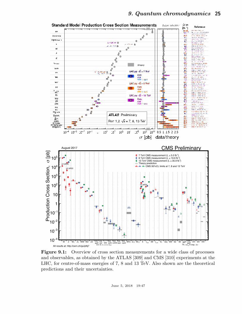
9. Quantum chromodynamics 25
RL dt
[fb�1] �e�erence
WZjj E�K 20.3 P�D 9�, �9���4 (���6)WWjj E�K 20.3 aXiv: �6�����4�8 �h p- x�Z�jj E�K 20.3 aXiv: �7�5���966 �h p- x�WW� 20.2 C��N-�P-���7-�96W�� 20.3 P�� ��5, ���8�� (���5)Z�� 20.3 P�D 9�, ������ (���6)Zjj E�K 20.3 JH�P �4, ��� (���4)3.2 C��N-�P-���7-��5Wjj E�K �.� aXiv:�7����4�6� �h p- x�20.2 aXiv:�7����4�6� �h p- x����� �.� P�D 9�, �7���7 (���5)
���Z 20.3 JH�P ��, �7� (���5)3.2 �PJC 77 (���7) 4����W 20.3 JH�P ��, �7� (���5)3.2 �PJC 77 (���7) 4��Zj 3�.� TOPQ-���6-�4WV �.� JH�P ��, �49 (���5)20.2 aXiv: �7�6���7�� �h p- x�Z� �.� P�D 87, ������ (����)20.3 P�D 9�, ������ (���6)W� �.� P�D 87, ������ (����)�s����� 20.3 P�B 756, ��8-�46 (���6)ZZ �.� JH�P ��, ��8 (����)20.3 JH�P ��, �99 (���7)3�.� AT�AS-CONF-���7-���WZ �.� �PJC 7�, ��7� (����)20.3 P�D 9�, �9���4 (���6)3.2 P�B 76� (���6) �W� 2.0 P�B 7�6, �4�-�59 (����)20.3 JH�P ��, �64 (���6)3.2 aXiv:�6����7��� �h p- x��� �.� JH�P ��, �86 (����)�� >!" #!!$ G%&
20.2 P�D 95 (���7) �����5�� >'* #+*$ G%&WW �.� P�D 87, ������ (����)20.3 P�B 76�, ��4 (���6)3.2 aXiv: �7����45�9 �h p- x��/����� �.� P�D 9�, �����6 (���4)20.3 aXiv:�7�����859 �h p- x�3.2 JH�P �4 (���7) �86
��� �.� �PJC 74: ���9 (���4)20.2 �PJC 74: ���9 (���4)3.2 P�B 76� (���6) ��6Z �.� JH�P �� (���7) ��720.2 JH�P �� (���7) ��73.2 JH�P �� (���7) ��7W �.� �PJC 77 (���7) �670.0;� P�B 759 (���6) 6���
�.� P�D 89, �5���4 (���4)< > =?? G%& 20.2 JH�P �6 (���6) ��5< > @I G%&3.2 P�B ���7 �4 �7�< > =@I G%&
MUjY�\ ^_`gk �.l JH�P �5, �59 (���4)3.2 AT�AS-CONF-���6-�9�mY�\ ^_`gk �.l JH�P ��, �5� (���5)20.2 aXiv: �7�6����9� �h p- x�3.2 AT�AS-CONF-���6-�9�
oo ;quwyz N{|}� Ph~�� B, 486-548 (���4)l0quwyz P�B 76� (���6) �58
� ����
���� ���� ���� ���� � ��� ��� ��� ��� ��� ��� ����
�����������
��� � ��� � ���
������
¡¢ ££¤¥ ¦ § ©ª
«¬¬®¯°¯®¯°¯ ± ®²®¯
¡¢ ££¤¥ ¦ ³ ©ª
«¬¬®¯°¯®¯°¯ ± ®²®¯
¡¢ ££¤¥ ¦ ´µ ©ª
«¬¬®¯°¯®¯°¯ ± ®²®¯
¶·¸¹º¸»º ¼½º¾¿ À»½ºÁ·ý¹ Ä»½ÅÅ ¶¾Â·Ã½¹ ¼¾¸ÅÁ»¾Æ¾¹·Å ǯ°¯È®É ÊÈ˲ ÌÍÎÏ
ÐÑÒÐÓ ÔÕÖ×ØÙØÚÛÕÜ
ÝÞÚ ßàáâ
ã ä åà æà ßç èéê
[p
b]
σP
rod
uctio
n C
ross S
ectio
n,
4−10
3−10
2−10
1−10
1
10
210
310
410
510
CMS PreliminaryAugust 2017
All results at: http://cern.ch/go/pNj7
W
n jet(s)≥
Z
n jet(s)≥
γW γZ WW WZ ZZ
µll, l=e,→, Zνl→EW: WqqWEW
qqZEW
WW
→γγ
γqqWEW
ssWW EW
γqqZEW
qqZZEW γWV γγZ γγW tt
=n jet(s)
t-cht tW
s-cht γtt tZq ttW ttZ tttt
σ∆ in exp. H
σ∆Th.
ggHqqHVBF VH ttH HH
CMS 95%CL limits at 7, 8 and 13 TeV
)-1 5.0 fb≤7 TeV CMS measurement (L )-1 19.6 fb≤8 TeV CMS measurement (L )-1 35.9 fb≤13 TeV CMS measurement (L
Theory prediction
Figure 9.1: Overview of cross section measurements for a wide class of processesand observables, as obtained by the ATLAS [309] and CMS [310] experiments at theLHC, for centre-of-mass energies of 7, 8 and 13 TeV. Also shown are the theoreticalpredictions and their uncertainties.
June 5, 2018 19:47
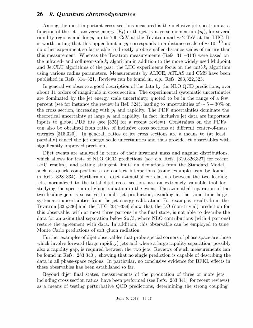
26 9. Quantum chromodynamics
Among the most important cross sections measured is the inclusive jet spectrum as afunction of the jet transverse energy (Et) or the jet transverse momentum (pt), for severalrapidity regions and for pt up to 700 GeV at the Tevatron and ∼ 2 TeV at the LHC. Itis worth noting that this upper limit in pt corresponds to a distance scale of ∼ 10−19 m:no other experiment so far is able to directly probe smaller distance scales of nature thanthis measurement. Whereas the Tevatron measurements (Refs. 311–313) were based onthe infrared- and collinear-safe kt algorithm in addition to the more widely used Midpointand JetCLU algorithms of the past, the LHC experiments focus on the anti-kt algorithmusing various radius parameters. Measurements by ALICE, ATLAS and CMS have beenpublished in Refs. 314–321. Reviews can be found in, e.g., Refs. 283,322,323.
In general we observe a good description of the data by the NLO QCD predictions, overabout 11 orders of magnitude in cross section. The experimental systematic uncertaintiesare dominated by the jet energy scale uncertainty, quoted to be in the range of a fewpercent (see for instance the review in Ref. 324), leading to uncertainties of ∼ 5− 30% onthe cross section, increasing with pt and rapidity. The PDF uncertainties dominate thetheoretical uncertainty at large pt and rapidity. In fact, inclusive jet data are importantinputs to global PDF fits (see [325] for a recent review). Constraints on the PDFscan also be obtained from ratios of inclusive cross sections at different center-of-massenergies [315,320]. In general, ratios of jet cross sections are a means to (at leastpartially) cancel the jet energy scale uncertainties and thus provide jet observables withsignificantly improved precision.
Dijet events are analyzed in terms of their invariant mass and angular distributions,which allows for tests of NLO QCD predictions (see e.g. Refs. [319,326,327] for recentLHC results), and setting stringent limits on deviations from the Standard Model,such as quark compositeness or contact interactions (some examples can be foundin Refs. 328–334). Furthermore, dijet azimuthal correlations between the two leadingjets, normalized to the total dijet cross section, are an extremely valuable tool forstudying the spectrum of gluon radiation in the event. The azimuthal separation of thetwo leading jets is sensitive to multi-jet production, avoiding at the same time largesystematic uncertainties from the jet energy calibration. For example, results from theTevatron [335,336] and the LHC [337–339] show that the LO (non-trivial) prediction forthis observable, with at most three partons in the final state, is not able to describe thedata for an azimuthal separation below 2π/3, where NLO contributions (with 4 partons)restore the agreement with data. In addition, this observable can be employed to tuneMonte Carlo predictions of soft gluon radiation.
Further examples of dijet observables that probe special corners of phase space are thosewhich involve forward (large rapidity) jets and where a large rapidity separation, possiblyalso a rapidity gap, is required between the two jets. Reviews of such measurements canbe found in Refs. [283,340], showing that no single prediction is capable of describing thedata in all phase-space regions. In particular, no conclusive evidence for BFKL effects inthese observables has been established so far.
Beyond dijet final states, measurements of the production of three or more jets,including cross section ratios, have been performed (see Refs. [283,341] for recent reviews),as a means of testing perturbative QCD predictions, determining the strong coupling
June 5, 2018 19:47
9. Quantum chromodynamics 27
constant (at NLO precision so far), and probing/tuning MC models, in particular thosecombining multi-parton matrix elements with parton showers.
In terms of precision achieved, measurements of inclusive vector boson (W, Z)production outperform the jet studies described above and provide the most preciselydetermined observables at hadron colliders so far. This is because the experimentalsignatures are based on leptons that are measured much more accurately than jets. Atthe LHC [342–348], the dominant uncertainty stems from the luminosity determination(∼2–4%), while other uncertainties (e.g. statistics, lepton efficiencies) are controlled atthe 1–3% level. The uncertainty from the acceptance correction of about 1–2% can bereduced by measuring so-called fiducial cross sections, ie. by applying kinematic cuts alsoto the particle level of the theoretical predictions. A further reduction or even completeelimination of particular uncertainties (e.g. luminosity) is achieved by measuring crosssection ratios (W/Z or W+/W−) or differential distributions that are normalised tothe inclusive cross section. On the theory side, as discussed earlier in this review, theproduction of these color-singlet states has been calculated up to NNLO accuracy. Sincethe dominant theoretical uncertainty is related to the choice of PDFs, these high-precisiondata provide useful handles for PDF determinations.
Further insights are obtained from measurements of differential vector bosonproduction, as a function of the invariant dilepton mass, the boson’s rapidity or itstransverse momentum. For example, the dilepton invariant mass distribution has beenmeasured [349–353] for masses between 15 and 2000 GeV, covering more than 8 orders ofmagnitude in cross section. NNLO QCD predictions, together with modern PDF sets andincluding higher-order electroweak and QED final-state radiation corrections, describethe data to within 5–10% over this large range, whereas NLO predictions show largerdeviations, unless matched to a parton shower.
Similar conclusions can be drawn from the observed rapidity distribution of the dileptonsystem (see e.g. [342,350]) or, in the case of W production, from the observed chargedlepton rapidity distribution and its charge asymmetry. The latter is particularly sensitiveto differences among PDF sets [342,354,355], also thanks to the high precision achievedby the ATLAS and CMS experiments for central rapidity ranges. These measurementsare nicely extended to the very forward region, up to 4.5 in lepton rapidity, by the LHCbexperiment.
An overview of this kind of measurements can be found in Ref. 283. There onecan also find a discussion of and references to LHC results from studies of the vectorboson’s transverse momentum distribution, pV
t (see also Refs. 356,357). This observableprobes different aspects of higher-order QCD effects and is sensitive to jet productionin association to the vector boson, without suffering from the large jet energy scaleuncertainties since there is no explicit jet reconstruction. Whereas in the pV
t region ofseveral tens to hundreds of GeV the NNLO predictions (that effectively are of NLOaccuracy for this variable) agree with the data to within about 10%, at transversemomentum below ∼5–10 GeV the fixed order predictions fail and soft-gluon resummationis needed to restore the agreement with data. Correspondingly, MC models implementingparton shower matching to LO or NLO matrix elements provide good predictions at lowand intermediate pV
t , but deviate up to 40% at high pVt .
June 5, 2018 19:47
28 9. Quantum chromodynamics
While in principle inclusive and differential photon production represents a similartool for studying effects as described above, the experimental results are less precisethan for W and Z production, related to the greater challenges encountered in photonreconstruction and purity determination compared to lepton final states.
In terms of complexity, probably the most challenging class of processes is vector boson(photon, W , Z) production together with jets. By now the amount of results obtainedboth at the Tevatron and at the LHC is so extensive that a comprehensive discussionwith a complete citation list would go much beyond the scope of this Review. We ratherrefer to recent summaries in Refs. 283,358 and to previous versions of this Review.
The measurements cover a very large phase space, e.g. with jet transverse momentabetween 30 GeV and ∼ 800 GeV and jet rapidities up to |y| < 4.4. Jet multiplicities ashigh as seven jets accompanying the vector boson have already been probed at the LHC,together with a substantial number of other kinematical observables, such as angularcorrelations among the various jets or among the jets and the vector boson, or the sumof jet transverse momenta, HT . Whereas the jet pt and HT distributions are dominatedby jet energy scale uncertainties at levels similar to those discussed above for inclusive jetproduction, angular correlations and jet multiplicity ratios have been measured with aprecision of ∼ 10%, see e.g. Refs. 359,275.
A general observation is that MC models, which implement a matching of matrix-element calculations with parton showers, provide a good description of the data withinuncertainties. Also NLO calculations for up to five jets [122] in addition to the vectorboson are in good agreement with the data over that phase space, where the calculationsare applicable; that is, one can not expect such predictions to work for, eg., the pt
distribution of the n + 1st jet with V + n jets calculated at NLO. However, with the highstatistics available to and the high precision achieved by the LHC experiments, some moredetailed observations can be made. MC models that implement parton shower matchingto LO matrix elements (LO+PS) tend to overpredict the data at large jet and/or bosonpt, while parton shower matching to NLO matrix elements gives better agreement. Theseproblems of LO+PS models are less acute when looking at angular correlations.
Also, electroweak corrections are expected to become more and more relevant nowthat the TeV energy range starts to be explored. For example, such corrections werefound [360] to be sizeable (tens of percent) when studying the ratio (dσγ/dpt)/(dσZ/dpt)in γ (Z)+jet production, pt being the boson’s transverse momentum, and might accountfor (some of) the differences observed in a CMS measurement [361] of this quantity.
The challenges get even more severe in the case of vector boson plus heavy quark(b, c) production, both because of theoretical issues (an additional scale is introduced bythe heavy quark mass and different schemes exist for the handling of heavy quarks andtheir mass effects in the initial and/or final state) and because of additional experimentaluncertainties related to the heavy-flavour tagging. A review of heavy quark productionat the LHC can be found in Ref. 362. There it is stated that studies of b-jet productionwith or without associated W and Z bosons reveal the di-b-jet pt and mass spectra to bewell modelled, within experimental and theoretical uncertainties, by most generators onthe market. However, sizeable differences between data and predictions are seen in themodelling of events with single b jets, particularly at large b-jet pt, where gluon splitting
June 5, 2018 19:47
9. Quantum chromodynamics 29
processes become dominant, as also confirmed by studies of b-hadron and b-jet angularcorrelations.
A number of interesting developments, in terms of probing higher-order QCD effects,have occurred in the sector of diboson production, in particular for the WW andγγ cases. Regarding the former, an early disagreement of about 10% between theLHC measurements and the NLO predictions had led to a number of speculations ofpossible new physics effects in this channel. However, more recent ATLAS and CMSmeasurements [363–365] are in agreement with the NNLO prediction [68].
In the case of diphoton production, ATLAS [366,367] and CMS [368] have providedaccurate measurements, in particular for phase-space regions that are sensitive to radiativeQCD corrections (multi-jet production), such as small azimuthal photon separation.While there are large deviations between data and NLO predictions in this region, acalculation [147] at NNLO accuracy manages to mostly fill this gap. This is an interestingexample where scale variations can not provide a reliable estimate of missing contributionsbeyond NLO, since at NNLO new channels appear in the initial state (gluon fusion inthis case).
In terms of heaviest particle involved, top-quark production at the LHC has becomean important tool for probing higher-order QCD calculations, thanks to very impressiveachievements both on the experimental and theoretical side, as extensively summarised inRef. 369. Regarding tt production, the most precise inclusive cross section measurementsare achieved using the dilepton (e µ) final state, with a total uncertainty of 4%. This is ofabout the same size as the uncertainty on the most advanced theoretical prediction [67],obtained at NNLO with additional soft-gluon resummation at NNLL accuracy. There isexcellent agreement between data and QCD prediction.
A large number of differential cross section measurements have been performed at7, 8 and 13 TeV centre-of-mass energy, studying distributions such as the top-quark pt
and rapidity, the transverse momentum and invariant mass of the tt system (probingscales up to the TeV range), or the number of additional jets. These measurements havebeen compared to a wide range of predictions, at fixed order up to NNLO as well asusing LO or NLO matrix elements matched to parton showers. While in general thereis good agreement observed with data, most MC simulations predict a somewhat hardertop-quark pt distribution than seen in data.
Thanks to both the precise measurements of and predictions for the inclusive top-paircross section, that is sensitive to the strong coupling constant and the top-quark mass,this observable has been used to measure the strong coupling constant at NNLO accuracyfrom hadron collider data [370,371] (cf. Section 9.4 below), as well as to obtain ameasurement of the top-quark’s pole mass without employing direct reconstructionmethods [370,372,373].
Finally, it is worth mentioning that steps are being undertaken towards using the newlyfound Higgs boson as a new tool for QCD studies, since Higgs production, dominatedby the gluon fusion process, is subject to very large QCD corrections. First studies offiducial and differential cross sections, using the ZZ, γγ and WW decay channels, havealready been performed [374–380], and the current experimental precision of ∼ 20% or
June 5, 2018 19:47
30 9. Quantum chromodynamics
more is expected to be substantially reduced with the future LHC data.
9.4. Determinations of the strong coupling constant
Beside the quark masses, the only free parameter in the QCD Lagrangian is the strongcoupling constant αs. The coupling constant in itself is not a physical observable, butrather a quantity defined in the context of perturbation theory, which enters predictionsfor experimentally measurable observables, such as R in Eq. (9.7).
Here, we retain the 2016 summary [381] of measurements of αs and extraction of theworld average value of αs(M
2Z), and leave an update of this section to a later version
of this Review ♯. This is done because only very few new results satisfying the selectioncriteria defined below were available at the deadline for this Review, while further newresults are expected to arrive (and actually have arrived) past-deadline.
Many experimental observables are used to determine αs. Considerations in suchdeterminations include:
• The observable’s sensitivity to αs as compared to the experimental precision.For example, for the e+e− cross section to hadrons (cf. R in Sec. 9.2.1), QCDeffects are only a small correction, since the perturbative series starts at orderα0
s ; 3-jet production or event shapes in e+e− annihilations are directly sensitiveto αs since they start at order αs; the hadronic decay width of heavy quarkonia,Γ(Υ → hadrons), is very sensitive to αs since its leading order term is ∝ α3
s .
• The accuracy of the perturbative prediction, or equivalently of the relation betweenαs and the value of the observable. The minimal requirement is generally consideredto be an NLO prediction. Some observables are predicted to NNLO (many inclusiveobservables, 3-jet rates and event shapes in e+e− collisions) or even N3LO (e+e−
hadronic cross section and τ branching fraction to hadrons). In certain cases,fixed-order predictions are supplemented with resummation. The precise magnitudeof theory uncertainties is usually estimated as discussed in Sec. 9.2.4.
• The size of non-perturbative effects. Sufficiently inclusive quantities, like the e+e−
cross section to hadrons, have small non-perturbative contributions ∼ Λ4/Q4.Others, such as event-shape distributions, have contributions ∼ Λ/Q.
• The scale at which the measurement is performed. An uncertainty δ on a measurementof αs(Q
2), at a scale Q, translates to an uncertainty δ′ = (α2s(M
2Z)/α2
s(Q2)) · δ on
αs(M2Z). For example, this enhances the already important impact of precise low-Q
measurements, such as from τ decays, in combinations performed at the MZ scale.
The selection of results from which to determine the world average value of αs(M2Z) is
restricted to those which are
- published in a peer-reviewed journal,
- based on the most complete perturbative QCD predictions, i.e. to those using NNLOor higher-order expansions.
♯ The time evolution of αs combinations can be followed by consulting Refs. [383–385]as well as earlier editions of this Review.
June 5, 2018 19:47
9. Quantum chromodynamics 31
This excludes e.g. results from jet production in DIS at HERA and at hadron colliderswhich are based on calculations at NLO only. These will nevertheless be discussed in thisreview, as they are important ingredients for the experimental evidence of the energydependence of αs, i.e. for Asymptotic Freedom, one of the key features of QCD. Notethat results which do not include reliable estimates of experimental, systematic andtheoretical uncertainties, which are based on not commonly accepted procedures like scaleoptimization, or which omit discussion or accounting of non-perturbative corrections andeffects, will not be referenced at all in this review.
In order to calculate the world average value of αs(M2Z), we apply an intermediate
step of pre-averaging results within certain sub-fields like e+e− annihilation, DIS andhadronic τ -decays, and calculate the overall world average from those pre-averages ratherthan from individual measurements. This is done because in most sub-fields one observesthat different determinations of the strong coupling from substantially similar datasetslead to values of αs that are only marginally compatible with each other, or with the finalworld average value, which presumably is a reflection of the challenges of evaluating andincluding appropriate systematic uncertainties.
So for each sub-field, the unweighted average of all selected results is taken as thepre-average value of αs(M
2Z), and the unweighted average of the quoted uncertainties
is assigned to be the respective overall error of this pre-average. However, if this errorappears to be smaller than the unweighted standard deviation - i.e. the spread - of theresults, the standard deviation is taken as the overall uncertainty instead. This is donein order to arrive at an unbiased estimator of the average value of αs(M
2Z) from this
sub-field, and to avoid that singular, optimistic estimates of systematic uncertaintiesdominate the field if these are not backed up by a broader consensus †.
Assuming that the resulting pre-averages are largely independent of each other, wedetermine the final world average value using the method of ‘χ2 averaging’, as proposed,e.g., in Ref. 386, in order to treat cases of possible (unknown) correlations as wellas possibly underestimated systematic uncertainties in a meaningful and well definedmanner: the central value is determined as the weighted average of the different inputvalues. An initial uncertainty of the central value is determined treating the uncertaintiesof all individual measurements as being uncorrelated and of Gaussian nature, and theoverall χ2 to the central value is calculated. If this initial χ2 is larger than the numberof degrees of freedom, then all individual uncertainties are enlarged by a common factorsuch that χ2/d.o.f. equals unity. If the initial value of χ2 is smaller than the numberof degrees of freedom, an overall correlation coefficient is introduced and determinedby requiring that the total χ2/d.o.f. equals unity. In both cases, the resulting overalluncertainty of αs is larger than the initial estimate of the uncertainty.
† In most practical cases, this procedure arrives at similar values as obtained from the‘range averaging’ method which we used in previous Reviews, while it avoids potentialshortcomings and biases of the latter.
June 5, 2018 19:47
32 9. Quantum chromodynamics
9.4.1. Hadronic τ decays :Based on complete N3LO predictions [35], analyses of the τ hadronic decay width andspectral functions have been performed, leading to precise determinations of αs at theenergy scale of M2
τ [35,387–393]. They are based on different approaches to treatperturbative and non-perturbative contributions, the impacts of which are a matter ofintense discussions, see e.g. [391] and [394].
In particular, there is a significant difference between results obtained using fixed-order(FOPT) or contour improved perturbation theory (CIPT), such that analyses based onCIPT generally arrive at about 7% larger values of αs(M
2τ ) than those based on FOPT.
When converted to αs(M2Z), the difference is about 2%. This uncertainty is about 5 times
larger than the typically achieved experimental precision. In addition, most recent resultsshow differences of up to 10% in αs(M
2τ ) (3% at MZ), between different groups using the
same data sets and perturbative calculations, most likely due to different treatments ofthe non-perturbative contributions, c.f. Ref. [393] with Refs. [391,392].
We determine the pre-average value of αs(M2Z) for this sub-field from studies which
employ both, FOPT and CIPT expansions, and which include the difference among these inthe quoted overall uncertainty: αs(M
2Z) = 0.1202±0.0019 [35], αs(M
2Z) = 0.1200±0.0015
[391], αs(M2Z) = 0.1199 ± 0.0015 [392], and αs(M
2Z) = 0.1165 ± 0.0019 [393].
We also include the result from τ decay and lifetime measurements, obtained inSec. Electroweak Model and constraints on New Physics of the 2013 edition of thisReview, αs(M
2Z) = 0.1193 ± 0.0023. All these are summarised in Fig. 9.2. Determining
the unweighted average of the central values and their overall uncertainties, we arrive atαs(M
2Z) = 0.1192 ± 0.0018 which we will use as the first input for determining the world
average value of αs(M2Z). This corresponds to αs(M
2τ ) = 0.325± 0.015 at the scale of the
τ -mass.
9.4.2. Lattice QCD :There are several current results on αs from lattice QCD, see also Sec. Lattice QCD
in this Review. The HPQCD collaboration [395] computes Wilson loops and similarshort-distance quantities with lattice QCD and analyzes them with NNLO perturbativeQCD. This yields a value for αs, but the lattice scale must be related to a physicalenergy/momentum scale. This is achieved with the Υ′-Υ mass difference, however, manyother quantities could be used as well [396]. HPQCD obtains αs(M
2Z) = 0.1184± 0.0006,
where the uncertainty includes effects from truncating perturbation theory, finite latticespacing and extrapolation of lattice data. An independent perturbative analysis of asubset of the same lattice-QCD data yields αs(M
2Z) = 0.1192 ± 0.0011 [397]. Using
another, independent methodology, the current-current correlator method, HPQCDobtains αs(M
2Z) = 0.1182 ± 0.0007 [395,398]. The analysis of Ref. 399, which uses
the Schroedinger functional scheme and avoids the staggered fermion treatment ofRef. 395, finds αs(M
2Z) = 0.1205 ± 0.0008 ± 0.0005 +0.0000
−0.0017, where the first uncertaintyis statistical and the others are from systematics. Since this approach uses a differentdiscretization of lattice fermions and a different general methodology, it providesan independent cross check of other lattice extractions of αs. A study of the ETMcollaboration [400] used lattice data with u, d, s and c quarks in the sea and examined the
June 5, 2018 19:47
9. Quantum chromodynamics 33
ghost-gluon coupling, obtaining αs(M2Z) = 0.1196 ± 0.0012. Finally, a determination of
αs from the QCD static potential [401] results in αs(M2Z) = 0.1166+0.0012
−0.0008. The JLQCDcollaboration, in an analysis of Adler functions, has recently corrected their initial resultof αs(M
2Z) = 0.1181+0.0014
−0.0012 downwards, by more than 5 standard deviations of their
assigned uncertainty, to αs(M2Z) = 0.1118+0.0016
−0.0017 [402]. For this and other reasonsdiscussed in [403], we do not include this result in our determination of the averagelattice result.
A summary of the results discussed above is given in Fig. 9.2. They average, applyingthe method of taking the unweighted averages of the central values and their quoteduncertainties at face value, to αs(M
2Z) = 0.1188 ± 0.0011, which we take as our second
result for the determination of the world average value of αs. This compares wellto a similar compilation and summary provided by the FLAG Working Group [403],suggesting αs(M
2Z) = 0.1184 ± 0.0012 as the overall average of lattice determinations of
αs. Both these error estimates are more conservative than the one (±0.0005) we used inour previous Review where we applied the χ2 averaging method.
9.4.3. Deep inelastic lepton-nucleon scattering (DIS) :Studies of DIS final states have led to a number of precise determinations of αs: acombination [404] of precision measurements at HERA, based on NLO fits to inclusivejet cross sections in neutral current DIS at high Q2, provides combined values of αs
at different energy scales Q, as shown in Fig. 9.3, and quotes a combined result ofαs(M
2Z) = 0.1198 ± 0.0032. A more recent study of multijet production [405], based on
improved reconstruction and data calibration, confirms the general picture, albeit witha somewhat smaller value of αs(M
2Z) = 0.1165 ± 0.0039, still in NLO. An evaluation of
inclusive jet production, including approximate NNLO contributions [406], reduces thetheoretical prediction for jet production in DIS, improves the description of the finalHERA data in particular at high photon virtuality Q2 and increases the central fit valueof the strong coupling constant.
Another class of studies, analyzing structure functions in NNLO QCD (and partlybeyond), provide results which serve as relevant inputs for the world average of αs. Mostof these studies do not, however, explicitly include estimates of theoretical uncertaintieswhen quoting fit results of αs. In such cases we add, in quadrature, half of the differencebetween the results obtained in NNLO and NLO to the quoted errors: A combinedanalysis of non-singlet structure functions from DIS [407], based on QCD predictionsup to N3LO in some of its parts, results in αs(M
2Z) = 0.1141 ± 0.0022 (BBG). Studies
of singlet and non-singlet structure functions, based on NNLO predictions, result inαs(M
2Z) = 0.1134 ± 0.0025 [408] (ABM) and in αs(M
2Z) = 0.1158 ± 0.0036 [409] (JR).
The MSTW group [410], also including data on jet production at the Tevatron,obtains, at NNLO♯♯, αs(M
2Z) = 0.1171 ± 0.0024. A recent update of this analysis,
also including hadron collider data, determined a new set of parton density functions(MMHT2014) [411], together with αs(M
2Z) = 0.1172 ± 0.0013. The NNPDF group [412]
♯♯ Note that for jet production at a hadron collider, only NLO predictions are available,while for the structure functions full NNLO was utilized.
June 5, 2018 19:47
34 9. Quantum chromodynamics
presented a result, αs(M2Z) = 0.1173 ± 0.0011, which is in line with the one from the
MMHT group, including rather small experimental and theoretical uncertainties of only6 and 9 per-mille, respectively.
We note that criticism has been expressed on some of the above extractions. Amongthe issues raised, we mention the neglect of singlet contributions at x ≥ 0.3 in purenon-singlet fits [413], the impact and detailed treatment of particular classes of data inthe fits [413,414], possible biases due to insufficiently flexible parametrizations of thePDFs [415] and the use of a fixed-flavor number scheme [416,417].
Summarizing the results from world data on structure functions, taking the unweighted
average of the central values and errors of all selected results, leads to a pre-average valueof αs(M
2Z) = 0.1156 ± 0.0021, see Fig. 9.2.
9.4.4. Heavy quarkonia decays :The latest extraction of the strong coupling constant from an analysis of radiative Υdecays [418] resulted in αs(M
2Z) = 0.119+0.006
−0.005. This determination is based on QCDat NLO only, so it will not be considered for the final extraction of the world averagevalue of αs; it is, however, an important ingredient for the demonstration of AsymptoticFreedom as given in Fig. 9.3.
9.4.5. Hadronic final states of e+
e− annihilations :
Re-analyses of event shapes in e+e− annihilation, measured around the Z peak andat LEP2 center-of-mass energies up to 209 GeV, using NNLO predictions matchedto NLL resummation and Monte Carlo models to correct for hadronization effects,resulted in αs(M
2Z) = 0.1224 ± 0.0039 (ALEPH) [419], with a dominant theoretical
uncertainty of 0.0035, and in αs(M2Z) = 0.1189 ± 0.0043 (OPAL) [420]. Similarly,
an analysis of JADE data [421] at center-of-mass energies between 14 and 46 GeVgives αs(M
2Z) = 0.1172 ± 0.0051, with contributions from hadronization model and from
perturbative QCD uncertainties of 0.0035 and 0.0030, respectively. Precise determinationsof αs from 3-jet production alone, in NNLO, resulted in αs(M
2Z) = 0.1175 ± 0.0025 [422]
from ALEPH data and in αs(M2Z) = 0.1199 ± 0.0059 [423] from JADE. These results are
summarized in the upper half of the e+e− sector of Fig. 9.2.
Another class of αs determinations is based on analytic calculations of non-perturbativeand hadronization effects, rather than on Monte Carlo models [424–427], using methodslike power corrections, factorization of soft-collinear effective field theory, dispersivemodels and low scale QCD effective couplings. In these studies, the world data on Thrustdistributions, or - most recently - C-parameter distributions, are analysed and fittedto perturbative QCD predictions in NNLO matched with resummation of leading logsup to N3LL accuracy, see Sec. 9.2.3.3. The results are αs(M
2Z) = 0.1164+0.0028
−0.0024 [424],
αs(M2Z) = 0.1135 ± 0.0011 [425] and αs(M
2Z) = 0.1137+0.0034
−0.0027 [426] from Thrust, and
αs(M2Z) = 0.1123 ± 0.0015 [427] from C-parameter. They are also displayed in Fig. 9.2.
Not to be included in the computation of the world average but worth mentioningare a computation of the NLO corrections to 5-jet production and comparison tothe measured 5-jet rates at LEP [428], giving αs(M
2Z) = 0.1156+0.0041
−0.0034, and acomputation of non-perturbative and perturbative QCD contributions to the scale
June 5, 2018 19:47
9. Quantum chromodynamics 35
evolution of quark and gluon jet multiplicities, including resummation, resulting inαs(M
2Z) = 0.1199 ± 0.0026 [429].
We note that there is criticism on both classes of αs extractions described above:those based on corrections of non-perturbative hadronization effects using QCD-inspiredMonte Carlo generators (since the parton level of a Monte Carlo simulation is not definedin a manner equivalent to that of a fixed-order calculation), as well as studies basedon non-perturbative analytic calculations, as their systematics have not yet been fullyverified. In particular, quoting rather small overall experimental, hadronization andtheoretical uncertainties of only 2, 5 and 9 per-mille, respectively [425,427], seemsunrealistic and has neither been met nor supported by other authors or groups.
In view of these open questions, the determination of the unweighted average anduncertainties is supposed to provide the most appropriate and unbiased estimate of theaverage value of αs(M
2Z) for this sub-field, which results in αs(M
2Z) = 0.1169 ± 0.0034.
9.4.6. Hadron collider results :Significant determinations of αs from data at hadron colliders, i.e. the Tevatron and theLHC, are obtained, however mostly still limited to QCD at NLO. At
√s = 1.96 TeV,
αs(M2Z) = 0.1161+0.0041
−0.0048 and
αs(M2Z) = 0.1191+0.0048
−0.0071
result from studies of inclusive jet cross sections [430] and from jet angular correla-tions [431], respectively. ATLAS data on inclusive jet production at
√s = 7 TeV [432]
lead to [433]αs(M
2Z) = 0.1151+0.0093
−0.0087 .
Here, experimental systematics, the choice of jet scale and the use of different PDFsdominate the large overall uncertainties. Determinations of αs from CMS data on theratio of inclusive 3-jet to 2-jet cross sections [434], from inclusive jet production [435]and from the 3-jet differential cross section [436] quoted values of
αs(M2Z) = 0.1148 ± 0.0014(exp.)+0.0053
−0.0023(theo.) ,
αs(M2Z) = 0.1185 ± 0.0019(exp.)+0.0060
−0.0037(theo.) and
αs(M2Z) = 0.1171 ± 0.0013(exp.)+0.0073
−0.0047(theo.) ,
respectively. Most recently, the ATLAS collaboration reported
αs(M2Z) = 0.1173 ± 0.0010(exp.)+0.0065
−0.0026(theo.) and
αs(M2Z) = 0.1195 ± 0.0018(exp.)+0.0062
−0.0022(theo.)
using the transverse energy-energy correlation function (TEEC) and its associatedazimuthal asymmetry (ATEEC), respectively [271]. All these results are at NLO only,however they provide valuable new values of αs at energy scales now extending up to1.4 TeV. Although not contributing to the overall world average of αs which we determine
June 5, 2018 19:47
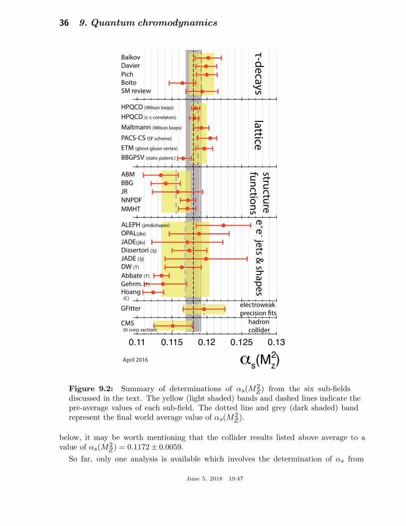
36 9. Quantum chromodynamics
τ-de
cays
lattice
structu
re
fun
ction
se
+e–
jets &
sha
pe
s
hadron
collider
electroweak
precision �ts
Baikov
ABM
BBG
JR
MMHT
NNPDF
Davier
Pich
Boito
SM review
HPQCD (Wilson loops)
HPQCD (c-c correlators)
Maltmann (Wilson loops)
Dissertori (3j)
JADE (3j)
DW (T)
Abbate (T)
Gehrm. (T)
CMS (tt cross section)
GFitter
Hoang (C)
JADE(j&s)
OPAL(j&s)
ALEPH (jets&shapes)
PACS-CS (SF scheme)
ETM (ghost-gluon vertex)
BBGPSV (static potent.)
April 2016
Figure 9.2: Summary of determinations of αs(M2Z) from the six sub-fields
discussed in the text. The yellow (light shaded) bands and dashed lines indicate thepre-average values of each sub-field. The dotted line and grey (dark shaded) bandrepresent the final world average value of αs(M
2Z).
below, it may be worth mentioning that the collider results listed above average to avalue of αs(M
2Z) = 0.1172 ± 0.0059.
So far, only one analysis is available which involves the determination of αs from
June 5, 2018 19:47
9. Quantum chromodynamics 37
hadron collider data in NNLO of QCD: from a measurement of the tt cross section at√s = 7 TeV, CMS [370] determined
αs(M2Z) = 0.1151+0.0028
−0.0027 ,
whereby the dominating contributions to the overall error are experimental (+0.0017−0.0018), from
parton density functions (+0.0013−0.0011) and the value of the top quark pole mass (±0.0013).
This latter result will enter our determination of the new world average of αs, andwill thereby open a new sub-field of αs determinations in this Review. We note, however,that so far there is only this one result in this sub-field. While there are more recentmeasurements of tt cross sections from ATLAS and from CMS, at
√s = 7, 8 and at
13 TeV, none quotes further extractions of αs. A more reliable result will thus be left tothe next Review, however we note that the most recent measurements of tt cross sectionsimply larger values of αs(M
2Z) than the one which we use, at this time, as result for this
sub-field.
9.4.7. Electroweak precision fit :The N3LO calculation of the hadronic Z decay width [35] was used in the latest updateof the global fit to electroweak precision data [437], resulting in
αs(M2Z) = 0.1196 ± 0.0030 ,
claiming a negligible theoretical uncertainty. We note that results from electroweakprecision data, however, strongly depend on the strict validity of Standard Modelpredictions and the existence of the minimal Higgs mechanism to implement electroweaksymmetry breaking. Any - even small - deviation of nature from this model could stronglyinfluence this extraction of αs.
9.4.8. Determination of the world average value of αs(M2Z) :
Obtaining a world average value for αs(M2Z) is a non-trivial exercise. A certain
arbitrariness and subjective component is inevitable because of the choice of measurementsto be included in the average, the treatment of (non-Gaussian) systematic uncertaintiesof mostly theoretical nature, as well as the treatment of correlations among the variousinputs, of theoretical as well as experimental origin.
We have chosen to determine pre-averages for sub-fields of measurements which areconsidered to exhibit a maximum of independence between each other, consideringexperimental as well as theoretical issues. The six pre-averages are summarized inFig. 9.2. We recall that these are exclusively obtained from extractions which are basedon (at least) full NNLO QCD predictions, and are published in peer-reviewed journals atthe time of completing this Review. These pre-averages are then combined to the finalworld average value of αs(M
2Z), using the χ2 averaging method and error treatment as
described above. From these, we determine the new world average value of
αs(M2Z) = 0.1181 ± 0.0011 , (9.23)
June 5, 2018 19:47
38 9. Quantum chromodynamics
with an uncertainty of 0.9 %.∗∗∗ This world average value is in reasonable agreementwith that from the 2013 version of this Review, which was αs(M
2Z) = 0.1185 ± 0.0006,
however at a somewhat decreased central value and with an overall uncertainty that hasalmost doubled. These changes are mainly due to the following developments:
- the uncertainty of the combined lattice result, now using the same averagingprocedure as applied to the other sub-fields, is more conservative than that used inour previous Review, leading to a larger final uncertainty of the new world average,and to a reduced fixing power towards the central average value;
- the relatively low value of αs from hadron collider results, which currently consistsof only one measurement of the tt cross section at
√s = 7 TeV [370] that is likely to
be a fluctuation to the low side.
For convenience, we also provide the values for ΛMS which correspond to the newworld average:
Λ(6)
MS= (89 ± 6) MeV, (9.24a)
Λ(5)
MS= (210 ± 14) MeV, (9.24b)
Λ(4)
MS= (292 ± 16) MeV, (9.24c)
Λ(3)
MS= (332 ± 17) MeV, (9.24d)
for nf = 6, 5, 4 and 3 quark flavors, which are determined using the 4-loop expressionfor the running of αs according to Eq. (9.5) and 3-loop matching at the charm-, bottom-and top-quark pole masses of 1.3, 4.2 and 173 GeV/c2, respectively. Note that for scalesbelow a few GeV, Eq. (9.5) starts to differ significantly from the exact solution of therenormalization group equation Eq. (9.3) and the latter is then to be preferred.
In order to further test and verify the sensitivity of the new average value of αs(M2Z)
to the different pre-averages and fields of αs determinations, we give each of the averagesobtained when leaving out one of the six input values, as well as the respective, initialvalue of χ2 :
αs(M2Z) = 0.1179± 0.0011 (w/o τ results; χ2
0/d.o.f. = 3.3/4), (9.25a)
αs(M2Z) = 0.1174± 0.0016 (w/o lattice results; χ2
0/d.o.f. = 2.9/4), (9.25b)
αs(M2Z) = 0.1185± 0.0013 (w/o DIS results; χ2
0/d.o.f. = 2.0/4), (9.25c)
αs(M2Z) = 0.1182± 0.0010 (w/o e+e− results; χ2
0/d.o.f. = 3.5/4), (9.25d)
αs(M2Z) = 0.1184± 0.0012 (w/o hadron collider; χ2
0/d.o.f. = 2.4/4) and (9.25e)
αs(M2Z) = 0.1180± 0.0010 (w/o e.w. precision fit; χ2
0/d.o.f. = 3.4/4). (9.25f)
∗∗∗ The weighted average, treating all inputs as uncorrelated measurements with Gaussianuncertainties, results in αs(M
2Z) = 0.11810 ± 0.00078 with χ2/d.o.f. = 3.7/5. Requiring
χ2/d.o.f. to reach unity calls for an overall correlation factor of 0.28, which increases theoverall uncertainty to ±0.00114.
June 5, 2018 19:47
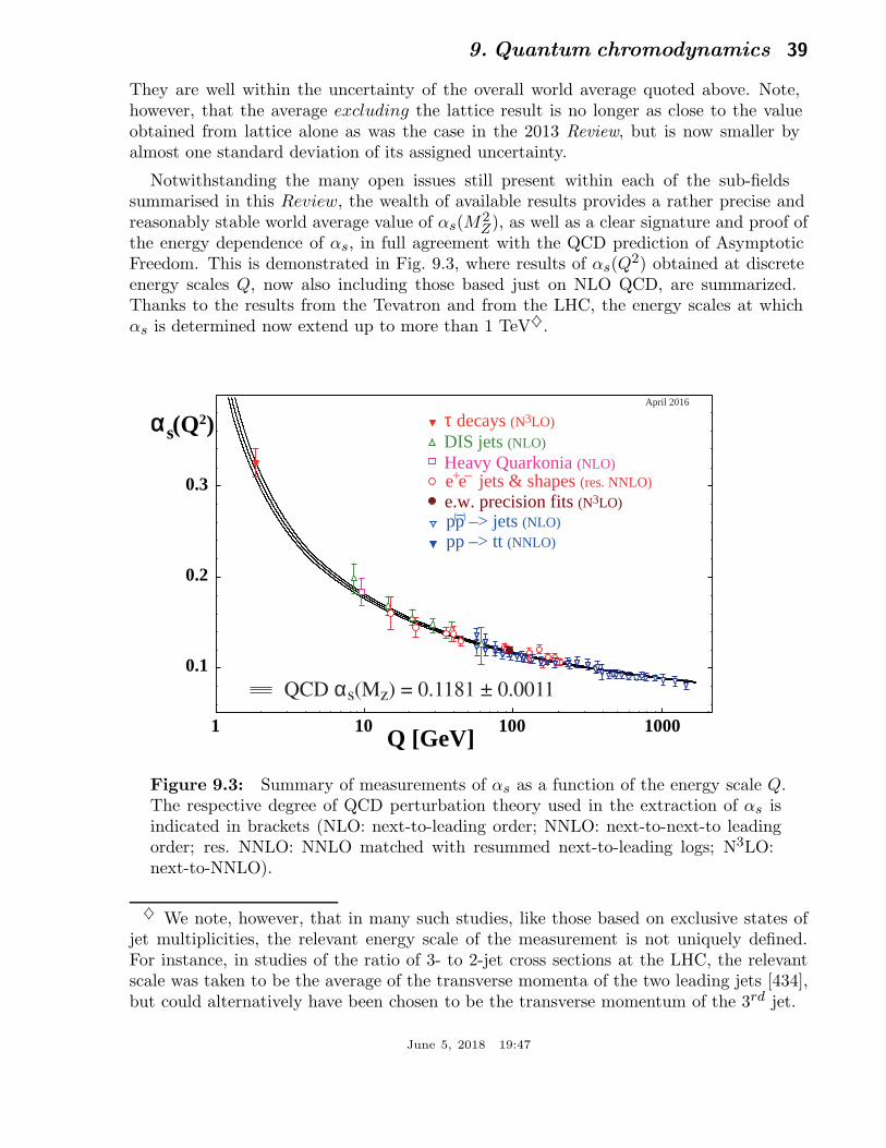
9. Quantum chromodynamics 39
They are well within the uncertainty of the overall world average quoted above. Note,however, that the average excluding the lattice result is no longer as close to the valueobtained from lattice alone as was the case in the 2013 Review, but is now smaller byalmost one standard deviation of its assigned uncertainty.
Notwithstanding the many open issues still present within each of the sub-fieldssummarised in this Review, the wealth of available results provides a rather precise andreasonably stable world average value of αs(M
2Z), as well as a clear signature and proof of
the energy dependence of αs, in full agreement with the QCD prediction of AsymptoticFreedom. This is demonstrated in Fig. 9.3, where results of αs(Q
2) obtained at discreteenergy scales Q, now also including those based just on NLO QCD, are summarized.Thanks to the results from the Tevatron and from the LHC, the energy scales at whichαs is determined now extend up to more than 1 TeV♦.
QCD αs(Mz) = 0.1181 ± 0.0011
pp –> jetse.w. precision fits (N3LO)
0.1
0.2
0.3
αs (Q2)
1 10 100Q [GeV]
Heavy Quarkonia (NLO)e+e– jets & shapes (res. NNLO)
DIS jets (NLO)
April 2016
τ decays (N3LO)
1000
(NLO
pp –> tt(NNLO)
)(–)
Figure 9.3: Summary of measurements of αs as a function of the energy scale Q.The respective degree of QCD perturbation theory used in the extraction of αs isindicated in brackets (NLO: next-to-leading order; NNLO: next-to-next-to leadingorder; res. NNLO: NNLO matched with resummed next-to-leading logs; N3LO:next-to-NNLO).
♦ We note, however, that in many such studies, like those based on exclusive states ofjet multiplicities, the relevant energy scale of the measurement is not uniquely defined.For instance, in studies of the ratio of 3- to 2-jet cross sections at the LHC, the relevantscale was taken to be the average of the transverse momenta of the two leading jets [434],but could alternatively have been chosen to be the transverse momentum of the 3rd jet.
June 5, 2018 19:47
40 9. Quantum chromodynamics
9.5. Acknowledgments
We are grateful to J.-F. Arguin, G. Altarelli, D. Britzger, J. Butterworth, M. Cacciari,L. del Debbio, D. d’Enterria, P. Gambino, C. Glasman Kuguel, N. Glover, M. Grazzini,A. Kronfeld, K. Kousouris, M. Luscher, Y. Ma, M. d’Onofrio, A. Ramos, S. Sharpe, R.Sommer, G. Sterman, D. Treille, N. Varelas, M. Wobisch, W.M. Yao, C.P. Yuan, and G.Zanderighi for discussions, suggestions and comments on this and earlier versions of thisReview.
References:
1. R.K. Ellis, W.J. Stirling, and B.R. Webber, “QCD and collider physics,” Camb.Monogr. Part. Phys. Nucl. Phys. Cosmol. 81 (1996).
2. C.A. Baker et al., Phys. Rev. Lett. 97, 131801 (2006).3. H.-Y. Cheng, Phys. Reports 158, 1 (1988).4. G. Dissertori, I.G. Knowles, and M. Schmelling, “High energy experiments and
theory,” Oxford, UK: Clarendon (2003).5. R. Brock et al., [CTEQ Collab.], Rev. Mod. Phys. 67, 157 (1995), see also
http://www.phys.psu.edu/~cteq/handbook/v1.1/handbook.pdf.6. A.S. Kronfeld and C. Quigg, Am. J. Phys. 78, 1081 (2010).7. T. Plehn, Lect. Notes Phys. 844, 1 (2012).8. J. Campbell, J. Huston, F. Krauss “The Black Book of Quantum Chromodynamics,
a Primer for the QCD Era,” Oxford University Press, UK (2017).9. R. Stock (Ed.), Relativistic Heavy Ion Physics, Springer-Verlag Berlin, Heidelberg,
2010.10. Proceedings of the XXIV International Conference on Ultrarelativistic Nucleus–
Nucleus Collisions, Quark Matter 2014, Nucl. Phys. A, volume 931.11. R. Hwa and X. N. Wang (Ed.), Quark Gluon Plasma 4, World Scientific Publishing
Company, 2010.12. T. van Ritbergen, J.A.M. Vermaseren, and S.A. Larin, Phys. Lett. B400, 379
(1997).13. M. Czakon, Nucl. Phys. B710, 485 (2005).14. P.A. Baikov, K.G. Chetyrkin, and J.H. Kuhn, Phys. Rev. Lett. 118, 082002 (2017).15. T. Luthe et al., JHEP 1607, 127 (2016).16. F. Herzog et al., JHEP 1702, 090 (2017).17. W.A. Bardeen et al., Phys. Rev. D18, 3998 (1978).
18. D.J. Gross and F. Wilczek, Phys. Rev. Lett. 30, 1343 (1973).19. H.D. Politzer, Phys. Rev. Lett. 30, 1346 (1973).20. Y. Schroder and M. Steinhauser, JHEP 0601, 051 (2006).21. K.G. Chetyrkin, J.H. Kuhn, and C. Sturm, Nucl. Phys. B744, 121 (2006).22. A.G. Grozin et al., JHEP 1109, 066 (2011).23. K.G. Chetyrkin, B.A. Kniehl, and M. Steinhauser, Nucl. Phys. B510, 61 (1998).24. M. Dalla Brida et al. [ALPHA Collaboration], Phys. Rev. Lett. 117, 182001 (2016).25. K.G. Chetyrkin, J.H. Kuhn, and M. Steinhauser, Comp. Phys. Comm. 133, 43
(2000).
June 5, 2018 19:47
9. Quantum chromodynamics 41
26. B. Schmidt and M. Steinhauser, Comp. Phys. Comm. 183, 1845 (2012)http://www.ttp.kit.edu/Progdata/ttp12/ttp12-02/.
27. F. Herren and M. Steinhauser, arXiv:1703.03751 [hep-ph].28. A.V. Bednyakov, Phys. Lett. B741, 262 (2015).29. M. Beneke, Phys. Reports 317, 1 (1999).30. P. Marquard et al., Phys. Rev. Lett. 114, 142002 (2015).31. P.A. Baikov et al., Phys. Lett. B714, 62 (2012).32. K.G. Chetyrkin, J.H. Kuhn, and A. Kwiatkowski, Phys. Reports 277, 189 (1996).33. Y. Kiyo et al., Nucl. Phys. B823, 269 (2009).34. P.A. Baikov et al., Phys. Rev. Lett. 108, 222003 (2012).35. P.A. Baikov, K.G. Chetyrkin, and J.H. Kuhn, Phys. Rev. Lett. 101, 012002 (2008).36. P.A. Baikov, K.G. Chetyrkin, and J.H. Kuhn, Phys. Rev. Lett. 96, 012003 (2006).37. P.A. Baikov and K.G. Chetyrkin, Phys. Rev. Lett. 97, 061803 (2006).38. F. Herzog et al., JHEP 1708, 113 (2017).39. D. Asner et al., arXiv:1307.8265 [hep-ex].40. H.W. Lin et al., Phys. Rev. D91, 054510 (2015);
C. Alexandrou et al., Phys. Rev. D92, 014502 (2015).41. G. C. Rossi and M. Testa, Phys. Rev. D96, 014507 (2017).42. J. Gao, L. Harland-Lang, and J. Rojo, arXiv:1709.04922 [hep-ph].43. J. D. Bjorken and E. A. Paschos, Phys. Rev. 185, 1975 (1969).44. J.A.M. Vermaseren, A. Vogt, and S. Moch, Nucl. Phys. B724, 3 (2005).45. S. Moch, J.A.M. Vermaseren, and A. Vogt, Nucl. Phys. B813, 220 (2009).46. J. Davies et al., PoS DIS 2016 (2016) 059.47. E. Laenen et al., Nucl. Phys. B392, 162 (1993);
S. Riemersma, J. Smith, and W.L. van Neerven, Phys. Lett. B347, 143 (1995).48. J. Blumlein, A. De Freitas, and C. Schneider, Nucl. Part. Phys. Proc. 261-262 185
Nucl. Part. Phys. Proc. 261-262 (2015) 185.49. J.C. Collins, D.E. Soper, and G.F. Sterman, Adv. Ser. Direct. High Energy Phys.
5, 1 (1988).50. J.C. Collins, Foundations of Perturbative QCD, Cambridge University Press, 2011.51. G.C. Nayak, J.-W. Qiu, and G.F. Sterman, Phys. Rev. D72, 114012 (2005).52. V.N. Gribov and L.N. Lipatov, Sov. J. Nucl. Phys. 15, 438 (1972);
L.N. Lipatov, Sov. J. Nucl. Phys. 20, 94 (1975);G. Altarelli and G. Parisi, Nucl. Phys. B126, 298 (1977);Yu.L. Dokshitzer, Sov. Phys. JETP 46, 641 (1977).
53. G. Curci, W. Furmanski, and R. Petronzio, Nucl. Phys. B175, 27 (1980);W. Furmanski and R. Petronzio, Phys. Lett. B97, 437 (1980).
54. A. Vogt, S. Moch, and J.A.M. Vermaseren, Nucl. Phys. B691, 129 (2004);S. Moch, J.A.M. Vermaseren, and A. Vogt, Nucl. Phys. B688, 101 (2004).
55. S. Moch et al., arXiv:1707.08315 [hep-ph].56. S. Moch, J.A.M. Vermaseren, and A. Vogt, Nucl. Phys. B889, 351 (2014).57. D. de Florian, G.F.R. Sborlini, and G. Rodrigo, Eur. Phys. J. C76, 282 (2016);
D. de Florian, G.F.R. Sborlini, and G. Rodrigo, JHEP 1610, 056 (2016).58. R.S. Thorne, Phys. Rev. D73, 054019 (2006).
June 5, 2018 19:47
42 9. Quantum chromodynamics
59. S. Forte et al., Nucl. Phys. B834, 116 (2010).60. M. Guzzi et al., Phys. Rev. D86, 053005 (2012).61. J.C. Collins, D.E. Soper, and G. Sterman, Nucl. Phys. B261, 104 (1985).62. R. Hamberg, W.L. van Neerven, and T. Matsuura, Nucl. Phys. B359, 343 (1991);
Erratum ibid., B 644 403, (2002).63. R.V. Harlander and W.B. Kilgore, Phys. Rev. Lett. 88, 201801 (2002).64. O. Brein, A. Djouadi, and R. Harlander, Phys. Lett. B579, 149 (2004).65. P. Bolzoni et al., Phys. Rev. Lett. 105, 011801 (2010).66. D. de Florian and J. Mazzitelli, Phys. Rev. Lett. 111, 201801 (2013).67. M. Czakon, P. Fiedler, and A. Mitov, Phys. Rev. Lett. 110, 252004 (2013).68. T. Gehrmann et al., Phys. Rev. Lett. 113, 21 (2014).69. F. Cascioli et al., Phys. Lett. B735, 311 (2014).70. C. Anastasiou et al., Phys. Rev. Lett. 114, 21 (2015);
C. Anastasiou et al., JHEP 1605, 058 (2016).71. F.A. Dreyer and A. Karlberg, Phys. Rev. Lett. 117, 072001 (2016).72. D. de Florian et al. [LHC Higgs Cross Section Working Group], arXiv:1610.07922
[hep-ph].73. M. Greco and A. Vicini, Nucl. Phys. B415, 386 (1994).74. L.N. Lipatov, Sov. J. Nucl. Phys. 23, 338 (1976) [Yad. Fiz. 23, 642 (1976)].75. E.A. Kuraev, L.N. Lipatov, and V.S. Fadin, Sov. Phys. JETP 45, 199 (1977) [Zh.
Eksp. Teor. Fiz. 72, 377 (1977)].76. I.I. Balitsky and L.N. Lipatov, Sov. J. Nucl. Phys. 28, 822 (1978) [Yad. Fiz. 28,
1597 (1978)].77. V.S. Fadin and L.N. Lipatov, Phys. Lett. B429, 127 (1998).78. M. Ciafaloni and G. Camici, Phys. Lett. B430, 329 (1998).79. G. Altarelli, R.D. Ball, and S. Forte, Nucl. Phys. B799, 199 (2008).80. M. Ciafaloni et al., JHEP 0708, 046 (2007).81. C.D. White and R.S. Thorne, Phys. Rev. D75, 034005 (2007).82. E. Iancu et al., Phys. Lett. B744, 293 (2015).83. N. Gromov, F. Levkovich-Maslyuk, and G. Sizov, arXiv:1507.04010 [hep-th];
V. N. Velizhanin, arXiv:1508.02857 [hep-th];S. Caron-Huot and M. Herranen, arXiv:1604.07417 [hep-ph].
84. I. Balitsky, Nucl. Phys. B463, 99 (1996).85. Y.V. Kovchegov, Phys. Rev. D60, 034008 (1999).86. A. Hebecker, Phys. Reports 331, 1 (2000).87. A.V. Belitsky and A.V. Radyushkin, Phys. Reports 418, 1 (2005).88. E. Boos et al., [CompHEP Collab.], Nucl. Instrum. Methods A534, 250 (2004)
http://comphep.sinp.msu.ru/.89. J. Alwall et al., JHEP 1407, 079 (2014), https://launchpad.net/mg5amcnlo.90. M.L. Mangano et al., JHEP 0307, 001 (2003), http://cern.ch/mlm/alpgen/.91. T. Gleisberg and S. Hoche, JHEP 0812, 039 (2008),
https://sherpa.hepforge.org/trac/wiki.92. A. Cafarella, C.G. Papadopoulos, and M. Worek, Comp. Phys. Comm. 180, 1941
(2009), http://cern.ch/helac-phegas/.
June 5, 2018 19:47
9. Quantum chromodynamics 43
93. F.A. Berends and W.T. Giele, Nucl. Phys. B306, 759 (1988).94. L.J. Dixon, arXiv:hep-ph/9601359.95. Z. Bern, L.J. Dixon, and D.A. Kosower, Ann. Phys. 322, 1587 (2007).96. S. Badger et al., Phys. Rev. D87, 3 (2013).97. S. Catani and M.H. Seymour, Nucl. Phys. B485, 291 (1997) [Erratum-ibid. B
510,503 (1998)].98. S. Frixione, Z. Kunszt, and A. Signer, Nucl. Phys. B467, 399 (1996).99. D.A. Kosower, Phys. Rev. D57, 5410 (1998);
J.M. Campbell, M.A. Cullen, and E.W.N. Glover, Eur. Phys. J. C9, 245 (1999);D.A. Kosower, Phys. Rev. D71, 045016 (2005).
100. Z. Nagy, Phys. Rev. D68, 094002 (2003), http://www.desy.de/~znagy/Site/
NLOJet++.html.101. J.M. Campbell and R.K. Ellis, Phys. Rev. D62, 114012 (2000).102. K. Arnold et al., arXiv:1107.4038 [hep-ph];
http://www-itp.particle.uni-karlsruhe.de/~vbfnloweb/.103. T. Binoth et al., Eur. Phys. J. C16, 311 (2000), http://lapth.in2p3.fr/
PHOX FAMILY/.104. G. Bevilacqua et al., Comp. Phys. Comm. 184, 986 (2013),
http://cern.ch/helac-phegas/.105. G. Cullen et al., Eur. Phys. J. C74, 8 (2014), http://gosam.hepforge.org/.106. S. Badger et al., Comp. Phys. Comm. 184, 1981 (2013),
https://bitbucket.org/njet/njet/wiki/Home.107. F. Cascioli, P. Maierhofer, and S. Pozzorini, Phys. Rev. Lett. 108, 111601 (2012),
https://openloops.hepforge.org/.108. S. Actis et al., Comp. Phys. Comm. 214, 140 (2017).109. T. Gleisberg et al., JHEP 0902, 007 (2009), http://projects.hepforge.org/
sherpa/.110. Z. Bern et al., PoS LL 2012,018 (2012).111. Z. Bern et al., Comp. Phys. Comm. 185, 1443 (2014).112. T. Kluge, K. Rabbertz, and M. Wobisch, arXiv:hep-ph/0609285,
http://fastnlo.hepforge.org/.113. T. Carli et al., Eur. Phys. J. C66, 503 (2010), https://applgrid.hepforge.org/.114. L. Del Debbio, N.P. Hartland, and S. Schumann, Comp. Phys. Comm. 185, 2115
(2014), http://mcgrid.hepforge.org/.115. V. Bertone et al., JHEP 1408, 166 (2014), https://amcfast.hepforge.org/.116. G. Cullen, N. Greiner, and G. Heinrich, Eur. Phys. J. C73, 4 (2013).117. S. Kallweit et al., JHEP 1504, 012 (2015).118. A. Denner et al., JHEP 1504, 018 (2015).119. S. Frixione et al., JHEP 1506, 184 (2015).120. R.K. Ellis et al., Phys. Reports 518, 141 (2012).121. S. Becker et al., Phys. Rev. Lett. 108, 032005 (2012).122. Z. Bern et al., Phys. Rev. D88, 014025 (2013).123. S. Badger et al., Phys. Rev. D89, 3 (2014).124. Z. Bern et al., Nucl. Phys. B425, 217 (1994).
June 5, 2018 19:47
44 9. Quantum chromodynamics
125. J.M. Campbell and E.W.N. Glover, Nucl. Phys. B527, 264 (1998).126. S. Catani and M. Grazzini, Phys. Lett. B446, 143 (1999).127. T. Binoth and G. Heinrich, Nucl. Phys. B585, 741 (2000).128. C. Anastasiou, K. Melnikov, and F. Petriello, Phys. Rev. D69, 076010 (2004).129. A. Gehrmann-De Ridder, T. Gehrmann, and E.W.N. Glover, JHEP 0509, 056
(2005).130. G. Somogyi, Z. Trocsanyi, and V. Del Duca, JHEP 0701, 070 (2007).131. M. Czakon, Phys. Lett. B693, 259 (2010).132. S. Catani and M. Grazzini, Phys. Rev. Lett. 98, 222002 (2007),
http://theory.fi.infn.it/grazzini/codes.html.133. R. Boughezal et al., Phys. Rev. Lett. 115, 6 (2015).134. J. Gaunt et al., arXiv:1505.04794 [hep-ph].135. M. Cacciari et al., arXiv:1506.02660 [hep-ph].136. A. Gehrmann-De Ridder et al., Phys. Rev. Lett. 99, 132002 (2007);
JHEP 0712, 094 (2007);Phys. Rev. Lett. 100, 172001 (2008).
137. A. Gehrmann-De Ridder et al., Comp. Phys. Comm. 185, 3331 (2014),https://eerad3.hepforge.org/.
138. S. Weinzierl, Phys. Rev. Lett. 101, 162001 (2008);JHEP 0906, 041 (2009).
139. J. Currie, T. Gehrmann, and J. Niehues, Phys. Rev. Lett. 117, 042001 (2016).140. K. Melnikov and F. Petriello, Phys. Rev. D74, 114017 (2006), http://gate.hep.
anl.gov/fpetriello/FEWZ.html.141. S. Catani et al., Phys. Rev. Lett. 103, 082001 (2009), http://theory.fi.infn.it/
grazzini/dy.html.142. C. Anastasiou, K. Melnikov, and F. Petriello, Nucl. Phys. B724, 197 (2005),
http://www.phys.ethz.ch/~pheno/fehipro/.143. S. Borowka et al., Phys. Rev. Lett. 117, 012001 (2016) Erratum:[Phys. Rev. Lett.
117, 079901 (2016).144. G. Ferrera, M. Grazzini, and F. Tramontano, Phys. Rev. Lett. 107, 152003 (2011).145. G. Ferrera, M. Grazzini, and F. Tramontano, Phys. Lett. B740, 51 (2015).146. M. Grazzini et al., JHEP 1705, 139 (2017).147. S. Catani et al., Phys. Rev. Lett. 108, 072001 (2012).148. J.M. Campbell et al., JHEP 1607, 148 (2016).149. M. Grazzini et al., Phys. Lett. B731, 204 (2014).150. M. Grazzini, S. Kallweit, and D. Rathlev, JHEP 1507, 085 (2015).151. R. Boughezal et al., Eur. Phys. J. C77, 7 (2017).152. R. Boughezal et al., arXiv:1504.07922 [hep-ph].153. R. Boughezal et al., Phys. Lett. B748, 5 (2015).154. F. Caola, K. Melnikov and M. Schulze, Phys. Rev. D92, 074032 (2015).155. X. Chen et al., JHEP 1610, 066 (2016).156. A. Gehrmann-De Ridder et al., Phys. Rev. Lett. 117, 022001 (2016).157. R. Boughezal et al., Phys. Rev. Lett. 116, 152001 (2016).158. J.M. Campbell, R.K. Ellis, and C. Williams, Phys. Rev. Lett. 118, 222001 (2017).
June 5, 2018 19:47
9. Quantum chromodynamics 45
159. M. Brucherseifer, F. Caola, and K. Melnikov, Phys. Lett. B736, 58 (2014).160. E.L. Berger et al., Phys. Rev. D94, 071501 (2016).161. M. Czakon, P. Fiedler, and A. Mitov, Phys. Rev. Lett. 115, 5 (2015).162. J. Currie, E.W.N. Glover, and J. Pires, Phys. Rev. Lett. 118, 072002 (2017).163. Y.L. Dokshitzer, D.Diakonov, and S.I. Troian, Phys. Reports 58, 269 (1980).164. G. Parisi and R. Petronzio, Nucl. Phys. B154, 427 (1979).165. G. Curci, M. Greco, and Y. Srivastava, Nucl. Phys. B159, 451 (1979).166. A. Bassetto, M. Ciafaloni, and G. Marchesini, Nucl. Phys. B163, 477 (1980).167. J.C. Collins and D.E. Soper, Nucl. Phys. B193, 381 (1981) [Erratum-ibid. B213,
545 (1983)].168. J.C. Collins and D.E. Soper, Nucl. Phys. B197, 446 (1982).169. J. Kodaira and L. Trentadue, Phys. Lett. B112, 66 (1982).170. J. Kodaira and L. Trentadue, Phys. Lett. B123, 335 (1983).171. J.C. Collins, D.E. Soper, and G. Sterman, Nucl. Phys. B250, 199 (1985).172. S. Catani et al., Nucl. Phys. B407, 3 (1993).173. C. W. Bauer et al., Phys. Rev. D63, 114020 (2001).174. C.W. Bauer, D. Pirjol, and I.W. Stewart, Phys. Rev. D65, 054022 (2002).175. T. Becher, A. Broggio, and A. Ferroglia, Lect. Notes Phys. 896 (2015) pp.1
arXiv:1410.1892 [hep-ph].176. S. Catani et al., Phys. Lett. B269, 432 (1991).177. N. Brown and W.J. Stirling, Phys. Lett. B252, 657 (1990).178. W. Bartel et al., [JADE Collab.], Z. Phys. C33, 23 (1986).179. N. Kidonakis, G. Oderda, and G. Sterman, Nucl. Phys. B531, 365 (1998).180. R. Bonciani et al., Phys. Lett. B575, 268 (2003).181. A. Banfi, G.P. Salam, and G. Zanderighi, JHEP 0503, 073 (2005).182. D. de Florian and M. Grazzini, Phys. Rev. Lett. 85, 4678 (2000).183. G. Bozzi et al., Nucl. Phys. B737, 73 (2006), http://theory.fi.infn.it/
grazzini/codes.html.184. G. Bozzi et al., Phys. Lett. B696, 207 (2011).185. T. Becher and M. Neubert, Eur. Phys. J. C71, 1665 (2011).186. T. Becher, M. Neubert, and D. Wilhelm, http://cute.hepforge.org/.187. D. de Florian et al., JHEP 1206, 132 (2012), http://theory.fi.infn.it/
grazzini/codes.html.188. C. Balazs and C.P. Yuan, Phys. Rev. D56, 5558 (1997).189. S. Catani et al., arXiv:1507.06937 [hep-ph].190. A. Banfi et al., Phys. Lett. B715, 152 (2012).191. M. Grazzini et al., arXiv:1507.02565 [hep-ph].192. D. de Florian and M. Grazzini, Nucl. Phys. B704, 387 (2005).193. T. Becher and G. Bell, JHEP 1211, 126 (2012).194. A. Banfi et al., Phys. Rev. Lett. 109, 202001 (2012);
T. Becher, M. Neubert, and L. Rothen, JHEP 1310, 125 (2013);I.W. Stewart et al., Phys. Rev. D89, 5 (2014).
195. I.W. Stewart, F.J. Tackmann, and W.J. Waalewijn, Phys. Rev. Lett. 106, 032001(2011).
June 5, 2018 19:47
46 9. Quantum chromodynamics
196. Y.-T. Chien et al., Phys. Rev. D87, 014010 (2013);T.T. Jouttenus et al., Phys. Rev. D88, 054031 (2013).
197. M. Dasgupta et al., JHEP 1210, 126 (2012).198. V. Ahrens et al., JHEP 1009, 097 (2010).199. M. Aliev et al., Comp. Phys. Comm. 182, 1034 (2011).200. N. Kidonakis, Phys. Rev. D82, 114030 (2010).201. T. Becher, C. Lorentzen, M. D. Schwartz, Phys. Rev. Lett. 108, 012001 (2012).202. T. Becher et al., Eur. Phys. J. C75, 4 (2015).203. E. Gerwick et al., JHEP 1502, 106 (2015).204. A. Banfi et al., JHEP 1505, 102 (2015).205. T. Becher and M.D. Schwartz, JHEP 0807, 034 (2008).206. A. H. Hoang et al., Phys. Rev. D91, 9 (2015).207. Y.-T. Chien and M.D. Schwartz, JHEP 1008, 058 (2010).208. P.F. Monni, T. Gehrmann, and G. Luisoni, JHEP 1108, 010 (2011).209. W. Bizon et al., arXiv:1705.09127 [hep-ph].210. S. Catani et al., Nucl. Phys. B888, 75 (2014).211. S. Fleming et al., Phys. Rev. D77, 074010 (2008).212. A.H. Hoang, P. Pietrulewicz, and D. Samitz, Phys. Rev. D93, 034034 (2016).213. I. Feige et al., Phys. Rev. Lett. 109, 092001 (2012).214. M. Dasgupta et al., JHEP 1309, 029 (2013).215. A.J. Larkoski et al., JHEP 1405, 146 (2014).216. M. Dasgupta, A. Powling, and A. Siodmok, arXiv:1503.01088 [hep-ph].217. A.J. Larkoski, I. Moult, and D. Neill, arXiv:1507.03018 [hep-ph].218. Yu.L. Dokshitzer et al., “Basics of perturbative QCD,” Gif-sur-Yvette, France:
Editions frontieres (1991), see also http://www.lpthe.jussieu.fr/~yuri/
BPQCD/cover.html.219. T. Sjostrand et al., Comp. Phys. Comm. 135, 238 (2001).220. T. Sjostrand, S. Mrenna, and P. Skands, JHEP 0605, 026 (2006),
http://projects.hepforge.org/pythia6/.221. T. Sjostrand et al., Comp. Phys. Comm. 191, 159 (2015),
http://home.thep.lu.se/~torbjorn/Pythia.html.222. B.R. Webber, Nucl. Phys. B238, 492 (1984).223. G. Corcella et al., JHEP 0101, 010 (2001), http://www.hep.phy.cam.ac.uk/
theory/webber/Herwig/.224. M. Bahr et al., Eur. Phys. J. C58, 639 (2008), http://projects.hepforge.org/
herwig/.225. L. Lonnblad, Comp. Phys. Comm. 71, 15, (1992).226. A. Buckley et al., Phys. Rept. 504, 145-233 (2011).227. B. Andersson et al., Phys. Reports 97, 31 (1983).228. T. Sjostrand, Nucl. Phys. B248, 469 (1984).229. T. Sjostrand and M. van Zijl, Phys. Rev. D36, 2019 (1987).230. S. Catani et al., JHEP 0111, 063 (2001).231. J. Alwall et al., Eur. Phys. J. C53, 473 (2008).232. S. Frixione and B.R. Webber, JHEP 0206, 029 (2002).
June 5, 2018 19:47
9. Quantum chromodynamics 47
233. P. Nason, JHEP 0411, 040 (2004).234. S. Alioli et al., JHEP 1006, 043 (2010), http://powhegbox.mib.infn.it/.235. S. Hoche et al., JHEP 1209, 049 (2012).236. S. Hoche et al., JHEP 1304, 027 (2013);
R. Frederix and S. Frixione, JHEP 1212, 061 (2012);S. Platzer, JHEP 1308, 114 (2013);L. Lonnblad and S. Prestel, JHEP 1303, 166 (2013);K. Hamilton et al., JHEP 1305, 082 (2013).
237. K. Hamilton et al., JHEP 1310, 222 (2013);A. Karlberg, E. Re, and G. Zanderighi, JHEP 1409, 134 (2014);S. Hoche, Y. Li and S. Prestel, Phys. Rev. D91, 074015 (2015);S. Hoche, Y. Li and S. Prestel, Phys. Rev. D90, 054011 (2014);S. Alioli et al., Phys. Rev. D92, 094020 (2015).
238. P.M. Stevenson, Phys. Lett. B100, 61 (1981).239. P.M. Stevenson, Phys. Rev. D23, 2916 (1981).240. G. Grunberg, Phys. Rev. D29, 2315 (1984).241. S.J. Brodsky, G.P. Lepage, and P.B. Mackenzie, Phys. Rev. D28, 228 (1983).242. M. Cacciari and N. Houdeau, JHEP 1109, 039 (2011).243. A. David and G. Passarino, Phys. Lett. B726, 266 (2013).244. E. Bagnaschi et al., JHEP 1502, 133 (2015).245. M. Cacciari et al., JHEP 0404, 068 (2004).246. M. Dasgupta and G.P. Salam, J. Phys. G30, R143 (2004).247. S. Moretti, L. Lonnblad, and T. Sjostrand, JHEP 9808, 001 (1998).248. G.P. Salam, Eur. Phys. J. C67, 637 (2010).249. S.D. Ellis et al., Prog. in Part. Nucl. Phys. 60, 484 (2008).250. M. Cacciari, Int. J. Mod. Phys. A30, 1546001 (2015).251. G.P. Salam and G. Soyez, JHEP 0705, 086 (2007).252. S. Catani et al., Nucl. Phys. B406, 187 (1993).253. S.D. Ellis and D.E. Soper, Phys. Rev. D48, 3160 (1993).254. Y.L. Dokshitzer et al., JHEP 9708, 001 (1997).255. M. Wobisch and T. Wengler, arXiv:hep-ph/9907280.256. M. Cacciari, G.P. Salam, and G. Soyez, JHEP 0804, 063 (2008).257. S. Bethke et al., Nucl. Phys. B370, 310 (1992), Nucl. Phys. B523, 681 (1998).258. M. Cacciari and G.P. Salam, Phys. Lett. B641, 57 (2006);
M. Cacciari, G.P. Salam, and G. Soyez, Eur. Phys. J. C72, 1896 (2012)http://fastjet.fr/.
259. S. Brandt et al., Phys. Lett. 12, 57 (1964).260. E. Farhi, Phys. Rev. Lett. 39, 1587 (1977).261. O. Biebel, Phys. Reports 340, 165 (2001).262. S. Kluth, Rept. on Prog. in Phys. 69, 1771 (2006).263. C.L. Basham et al., Phys. Rev. Lett. 41, 1585 (1978).264. A. Ali, E. Pietarinen, and W. J. Stirling, Phys. Lett. B141, 447 (1984).265. I. W. Stewart, F. J. Tackmann, and W. J. Waalewijn, Phys. Rev. Lett. 105, 092002
(2010).
June 5, 2018 19:47
48 9. Quantum chromodynamics
266. A. Banfi, G.P. Salam, and G. Zanderighi, JHEP 0408, 062 (2004).267. A. Banfi, G.P. Salam, and G. Zanderighi, JHEP 1006, 038 (2010).268. T. Aaltonen et al., [CDF Collab.], Phys. Rev. D83, 112007 (2011).269. G. Aad et al., [ATLAS Collab.], Eur. Phys. J. C72, 2211 (2012).270. G. Aad et al., [ATLAS Collab.], Phys. Rev. D88, 032004 (2013).271. G. Aad et al., [ATLAS Collab.], Phys. Lett. B750, 427 (2015).272. G. Aad et al., [ATLAS Collab.], Eur. Phys. J. C76, 375 (2016).273. M. Aaboud et al., [ATLAS Collab.], arXiv:1707.02562 [hep-ex].274. V. Khachatryan et al., [CMS Collab.], Phys. Lett. B699, 48 (2011).275. S. Chatrchyan et al., [CMS Collab.], Phys. Lett. B722, 238 (2013).276. V. Khachatryan et al., [CMS Collab.], JHEP 1410, 87 (2014).277. S. Chatrchyan et al., [CMS Collab.], Phys. Lett. B730, 243 (2014).278. G. Aad et al., [ATLAS Collab.], Phys. Rev. D83, 052003 (2011).279. S. Chatrchyan et al., [CMS Collab.], JHEP 1206, 160 (2012).280. B. B. Abelev et al., [ALICE Collab.], Phys. Rev. D91, 112012 (2015).281. G. Aad et al., [ATLAS Collab.], Eur. Phys. J. C73, 2676 (2013).282. C. Glasman [H1 Collab. and ZEUS Collab.], Nucl. Phys. (Proc. Supp.) 191, 121
(2009).283. T. Carli, K. Rabbertz, and S. Schumann, arXiv:1506.03239 [hep-ex].284. A. Abdesselam et al., Eur. Phys. J. C71, 1661 (2011).285. A. Altheimer et al., J. Phys. G39, 063001 (2012).286. A. Altheimer et al., Eur. Phys. J. C74, 2792 (2014).287. S. Schaetzel, Eur. Phys. J. C75, 9 (2015).288. A. J. Larkoski, I. Moult, and B. Nachman, arXiv:1709.04464 [hep-ph].289. D. Adams et al., Eur. Phys. J. C75, 409 (2015).290. T. Schorner-Sadenius, Eur. Phys. J. C72, 2060 (2012).291. J.M. Campbell, J.W. Huston, and W.J. Stirling, Rept. on Prog. in Phys. 70, 89
(2007).292. M.L. Mangano, Phys. Usp. 53, 109 (2010).293. J.M. Butterworth, G. Dissertori, and G.P. Salam, Ann. Rev. Nucl. and Part. Sci.
62, 387 (2012).294. T. Carli, T. Gehrmann, and S. Hoche, Eur. Phys. J. C67, 73 (2010).295. F.D. Aaron et al., [H1 Collab.], Eur. Phys. J. C65, 363 (2010).296. F.D. Aaron et al., [H1 Collab.], Eur. Phys. J. C54, 389 (2008).297. S. Chekanov et al., [ZEUS Collab.], Eur. Phys. J. C52, 515 (2007).298. S. Chekanov et al., [ZEUS Collab.], Phys. Rev. D78, 032004 (2008).299. H. Abramowicz et al., [ZEUS Collab.], Eur. Phys. J. C70, 965 (2010).300. H. Abramowicz et al., [ZEUS Collab.], Phys. Lett. B691, 127 (2010).301. S. Chekanov et al., [ZEUS Collab.], Phys. Rev. D85, 052008 (2012).302. F.D. Aaron et al., [H1 Collab.], Eur. Phys. J. C67, 1 (2010).303. V. Andreev et al., [H1 Collab.], Eur. Phys. J. C75, 2 (2015).304. S. Chekanov et al., [ZEUS Collab.], Nucl. Phys. B792, 1 (2008).305. S. Chekanov et al., [ZEUS Collab.], Phys. Rev. D76, 072011 (2007).306. A. Aktas et al., [H1 Collab.], Phys. Lett. B639, 21 (2006).
June 5, 2018 19:47
9. Quantum chromodynamics 49
307. H. Abramowicz et al., [ZEUS Collab.], Eur. Phys. J. C71, 1659 (2011).308. H. Abramowicz et al., [ZEUS Collab.], Nucl. Phys. B864, 1 (2012).309. http://atlas.web.cern.ch/Atlas/GROUPS/PHYSICS/
CombinedSummaryPlots/SM.310. http://twiki.cern.ch/twiki/bin/view/CMSPublic/PhysicsResultsCombined.311. A. Abulencia et al., [CDF - Run II Collab.], Phys. Rev. D75, 092006 (2007)
[Erratum-ibid. 119901].312. V.M. Abazov et al., [D0 Collab.], Phys. Rev. Lett. 101, 062001 (2008).313. V.M. Abazov et al., [D0 Collab.], Phys. Rev. D85, 052006 (2012).314. B. Abelev et al., [ALICE Collab.], Phys. Lett. B722, 262 (2013).315. G. Aad et al., [ATLAS Collab.], Eur. Phys. J. C73, 2509 (2013).316. G. Aad et al., [ATLAS Collab.], JHEP 1502, 153 (2015), erratum JHEP 1509, 141
(2015).317. M. Aaboud et al., [ATLAS Collab.], JHEP 1709, 020 (2017).318. V. Khachatryan et al., [CMS Collab.], Eur. Phys. J. C76, 265 (2016).319. S. Chatrchyan et al., [CMS Collab.], Phys. Rev. D87, 112002 (2013).320. V. Khachatryan et al., [CMS Collab.], JHEP 1703, 156 (2017).321. V. Khachatryan et al., [CMS Collab.], Eur. Phys. J. C76, 451 (2016).322. M. Wobisch et al., [fastNLO Collab.], arXiv:1109.1310 [hep-ph].323. P. Francavilla, Int. J. Mod. Phys. A30, 1546003 (2015).324. A. Schwartzman, Int. J. Mod. Phys. A30, 1546002 (2015).325. J. Rojo, Int. J. Mod. Phys. A30, 1546005 (2015).326. G. Aad et al., [ATLAS Collab.], JHEP 1405, 059 (2014).327. A. M. Sirunyan et al., [CMS Collab.], arXiv:1705.02628 [hep-ex].328. T. Aaltonen et al., [CDF Collab.], Phys. Rev. D79, 112002 (2009).329. V.M. Abazov et al., [D0 Collab.], Phys. Rev. Lett. 103, 191803 (2009).330. S. Chatrchyan et al., [CMS Collab.], JHEP 1205, 055 (2012).331. V. Khachatryan et al., [CMS Collab.], Phys. Lett. B746, 79 (2015).332. A.M. Sirunyan et al., [CMS Collab.], JHEP 1707, 013 (2017).333. G. Aad et al., [ATLAS Collab.], JHEP 1301, 029 (2013).334. M. Aaboud et al., [ATLAS Collab.], arXiv:1703.09127 [hep-ex].335. V.M. Abazov et al., [D0 Collab.], Phys. Rev. Lett. 94, 221801 (2005).336. V.M. Abazov et al., [D0 Collab.], Phys. Lett. B721, 212 (2013).337. G. Aad et al., [ATLAS Collab.], Phys. Rev. Lett. 106, 172002 (2011).338. V. Khachatryan et al., [CMS Collab.], Phys. Rev. Lett. 106, 122003 (2011).339. V. Khachatryan et al., [CMS Collab.], Eur. Phys. J. C76, 536 (2016).340. M. Campanelli, Int. J. Mod. Phys. A30, 1546006 (2015).341. P. Kokkas, Int. J. Mod. Phys. A30, 1546004 (2015).342. M. Aaboud et al., [ATLAS Collab.], Eur. Phys. J. C77, 367 (2017).343. G. Aad et al. et al., [ATLAS Collab.], Phys. Lett. B759, 601 (2016).344. S. Chatrchyan et al., [CMS Collab.], JHEP 1110, 132 (2011).345. S. Chatrchyan et al., [CMS Collab.], Phys. Rev. Lett. 112, 191802 (2014).346. R. Aaij et al., [LHCb Collab.], JHEP 1206, 058 (2012).347. R. Aaij et al., [LHCb Collab.], JHEP 1601, 155 (2016).
June 5, 2018 19:47
50 9. Quantum chromodynamics
348. R. Aaij et al., [LHCb Collab.], JHEP 1609, 136 (2016).349. S. Chatrchyan et al., [CMS Collab.], JHEP 1110, 007 (2011).350. V. Khachatryan et al., [CMS Collab.], Eur. Phys. J. C75, 147 (2015).351. G. Aad et al., [ATLAS Collab.], Phys. Lett. B725, 223 (2013).352. G. Aad et al., [ATLAS Collab.], JHEP 1406, 112 (2014).353. G. Aad et al., [ATLAS Collab.], JHEP 1608, 009 (2016).354. S. Chatrchyan et al., [CMS Collab.], Phys. Rev. D90, 3 (2014).355. V. Khachatryan et al., [CMS Collab.], Eur. Phys. J. C76, 469 (2016).356. G. Aad et al., [ATLAS Collab.], Eur. Phys. J. C76, 291 (2016).357. V. Khachatryan et al., [CMS Collab.], JHEP 1702, 096 (2017).358. U. Blumenschein, Int. J. Mod. Phys. A30, 1546007 (2015).359. G. Aad et al., [ATLAS Collab.], JHEP 1307, 032 (2013).360. J. H. Kuhn et al., JHEP 0603, 059 (2006).361. V. Khachatryan et al., [CMS Collab.], JHEP 1510, 128 (2015), erratum JHEP
1604, 010 (2016).362. M. Voutilainen, Int. J. Mod. Phys. A30, 1546008 (2015).363. G. Aad et al., [ATLAS Collab.], JHEP 1609, 029 (2016).364. M. Aaboud et al., [ATLAS Collab.], Phys. Lett. B773, 354 (2017).365. V. Khachatryan et al., [CMS Collab.], Eur. Phys. J. C76, 401 (2016).366. G. Aad et al., [ATLAS Collab.], JHEP 1301, 086 (2013).367. M. Aaboud et al., [ATLAS Collab.], Phys. Rev. D95, 112005 (2017).368. S. Chatrchyan et al., [CMS Collab.], Eur. Phys. J. C74, 3129 (2014).369. K. Kroninger, A. B. Meyer, and P. Uwer, arXiv:1506.02800 [hep-ex].370. S. Chatrchyan et al., [CMS Collab.], Phys. Lett. B728, 496 (2014), Phys. Lett.
B728, 526 (2014).371. T. Klijnsma, S. Bethke, G. Dissertori, and G. P. Salam, arXiv:1708.07495
[hep-ph].372. G. Aad et al., [ATLAS Collab.], Eur. Phys. J. C74, 10 (2014).373. A.M. Sirunyan et al., [CMS Collab.], JHEP 1709, 051 (2017).374. G. Aad et al., [ATLAS Collab.], Phys. Rev. Lett. 115, 091801 (2015).375. G. Aad et al., [ATLAS Collab.], JHEP 1608, 104 (2016).376. M. Aaboud et al., [ATLAS Collab.], arXiv:1708.02810 [hep-ex].377. S. Chatrchyan et al., [CMS Collab.], Phys. Rev. D89, 9 (2014).378. V. Khachatryan et al., [CMS Collab.], Eur. Phys. J. C76, 13 (2016).379. V. Khachatryan et al., [CMS Collab.], JHEP 1604, 005 (2016).380. V. Khachatryan et al., [CMS Collab.], JHEP 1703, 032 (2017).381. S. Bethke, G. Dissertori and G.P. Salam in [382].382. C. Patrignani et al., [Particle Data Group Collaboration], Chin. Phys. C40 (2016)
100001.383. S. Bethke, Prog. in Part. Nucl. Phys. 58, 351 (2007).384. S. Bethke, Eur. Phys. J. C64, 689 (2009).385. S. Bethke, J. Phys. G26, R27 (2000).386. M. Schmelling, Phys. Scripta 51, 676 (1995).387. M. Beneke and M. Jamin, JHEP 0809, 044 (2008).
June 5, 2018 19:47
9. Quantum chromodynamics 51
388. K. Maltman and T. Yavin, Phys. Rev. D78, 094020 (2008).389. S. Narison, Phys. Lett. B673, 30 (2009).390. I. Caprini and J. Fischer, Eur. Phys. J. C64, 35 (2009).391. A. Pich, Prog. in Part. Nucl. Phys. 75, 41 (2014).392. M. Davier et al., Eur. Phys. J. C74, 2803 (2014).393. D. Boito et al., Phys. Rev. D 91,034003(2015).394. G. Altarelli, PoS Corfu 2012 (2013) 002.395. C. McNeile et al., [HPQCD Collab.], Phys. Rev. D82, 034512 (2010).396. C.T.H. Davies et al., [HPQCD Collab., UKQCD Collab., and MILC Collab.], Phys.
Rev. Lett. 92, 022001 (2004).397. K. Maltman et al., Phys. Rev. D78, 114504 (2008).398. B. Chakraborty et al., [HPQCD Collab.], Phys. Rev. D91, 054508 (2015).399. S. Aoki et al., [PACS-CS Collab.], JHEP 0910, 053 (2009).400. B. Blossier et al., [ETM Collab.], Phys. Rev. Lett. 108, 262002 (2012), Phys. Rev.
D89, 014507 (2014).401. A. Bazavov et al., [BBGPSV], Phys. Rev. D90, 074038 (2014).402. E. Shintani et al., [JLQCD Collab.], Phys. Rev. D82, 074505 (2010), erratum Phys.
Rev. D89, 099903 (2014).403. S. Aoki et al., Eur. Phys. J. C74, 2890 (2014).404. C. Glasman [H1 Collab. and ZEUS Collab.], J. Phys. Conf. Ser. 110 022013 (2008).405. V. Andreev et al., (H1 Collab.), Eur. Phys. J. C75, 65 (2015).406. T. Biekotter, M. Klasen and G. Kramer, Phys. Rev. D92, 074037 (2015).407. J. Blumlein, H. Bottcher, and A. Guffanti, Nucl. Phys. B774, 182 (2007).408. S. Alekhin, J. Blumlein, and S. Moch, Phys. Rev. D86, 054009 (2012).409. P. Jimenez-Delgado and E. Reya, Phys. Rev. D79, 074023 (2009).410. A. D. Martin et al., Eur. Phys. J. C64, 653 (2009).411. L. A. Harland-Lang et al., Eur. Phys. J. C75, 435 (2015).412. R.D. Ball et al., Phys. Lett. B707, 66 (2012).413. R.S. Thorne and G. Watt, JHEP 1108, 100 (2011).414. S. Alekhin, J. Blumlein, and S.Moch, Eur. Phys. J. C71, 1723 (2011).415. R.D. Ball et al., Phys. Lett. B704, 36 (2011).416. R.D. Ball et al., Phys. Lett. B723, 330 (2013).417. R.S. Thorne et al., PoS DIS 2013 (2013) 042.418. N. Brambilla et al., Phys. Rev. D75, 074014 (2007).419. G. Dissertori et al., JHEP 0908, 036 (2009).420. G. Abbiendi et al., Eur. Phys. J. C71, 1733 (2011).421. S. Bethke et al., [JADE Collab.], Eur. Phys. J. C64, 351 (2009).422. G. Dissertori et al., Phys. Rev. Lett. 104, 072002 (2010).423. J. Schieck et al., Eur. Phys. J. C73, 2332 (2013).424. R.A. Davison and B.R. Webber, Eur. Phys. J. C59, 13 (2009).425. R. Abbate et al., Phys. Rev. D83, 074021 (2011).426. T. Gehrmann et al., Eur. Phys. J. C73, 2265 (2013).427. A.H. Hoang et al., Phys. Rev. D91, 094018 (2015).428. R. Frederix et al., JHEP 1011, 050 (2010).
June 5, 2018 19:47
52 9. Quantum chromodynamics
429. P. Bolzoni, B.A. Kniehl, and A.V. Kotikov, Nucl. Phys. B875, 18 (2013).430. M. Abazov et al., [D0 Collab.], Phys. Rev. D80, 111107 (2009).431. M. Abazov et al., [D0 Collab.], Phys. Lett. B718, 56 (2012).432. G. Aad et al., [ATLAS Collab.], Phys. Rev. D86, 014022 (2012).433. B. Malaescu and P. Starovoitov, Eur. Phys. J. C72, 2041 (2012).434. S. Chatrchyan et al., [CMS Collab.], Eur. Phys. J. C73, 2604 (2013).435. V. Khachatryan et al., [CMS Collab.], Eur. Phys. J. C75, 288 (2015).436. V. Khachatryan et al., [CMS Collab.], Eur. Phys. J. C75, 186 (2015).437. M. Baak et al., [Gfitter group], Eur. Phys. J. C74, 3046 (2014).
June 5, 2018 19:47


![arXiv:math/0110288v1 [math.NT] 26 Oct 2001 · The calculation of the singular Fourier coefficients uses extensively ideas from [10], where the case of n= pwas considered. However,](https://static.fdocument.org/doc/165x107/5fc3b3f1199f32581a09655e/arxivmath0110288v1-mathnt-26-oct-2001-the-calculation-of-the-singular-fourier.jpg)