9 Pulse Measurement
55
ETH Zurich Ultrafast Laser Physics Ursula Keller / Lukas Gallmann ETH Zurich, Physics Department, Switzerland www.ulp.ethz.ch Chapter 9: Pulse measurement Ultrafast Laser Physics
-
Upload
alexander-sukhov -
Category
Documents
-
view
234 -
download
0
Transcript of 9 Pulse Measurement

ETH Zurich Ultrafast Laser Physics
Ursula Keller / Lukas Gallmann
ETH Zurich, Physics Department, Switzerland www.ulp.ethz.ch
Chapter 9: Pulse measurement
Ultrafast Laser Physics

Ultrashort optical pulse
E(t ) = A(t)eiϕ ( t)e−iω 0t E(ω) = A(ω )eiϕ (ω )Time-domain! Frequency-domain!
Fourier transforms!
-1.0
-0.5
0.0
0.5
1.0
-30 -20 -10 0 10 20 30Time (fs)
1.0
0.8
0.6
0.4
0.2
0.0
-30 -20 -10 0 10 20 30Time (fs)
τp
I( t) = E(t)2 I(ω ) = E(ω )2
τ p ∝1Δω
Δω ∝ 1τ p
1.0
0.8
0.6
0.4
0.2
0.0
3.02.82.62.42.22.01.8Frequency (fs-1)
Δω

Cables and connectors
Connector type Frequency region Compatibility
BNC (Bayonet Navy Connector) DC – 2 GHz
SMC (Sub-Miniature C) DC – 7 GHz
APC-7 (Amphenol Precision Connector) DC – 18 GHz
Type N (Navy) 50 DC – 18 GHz
SMA (Sub-Miniature A) DC – 24 GHz 3.5 mm, 2.92 mm, Wiltron K
3.5 mm DC – 34 GHz SMA, 2.92 mm, Wiltron K
2.92 mm or Wiltron K DC – 40 GHz SMA, 3.5 mm
2.4 mm DC – 50 GHz 1.85 mm, Wiltron V
1.85 mm or Wiltron V DC – 65 GHz 2.4 mm
BNC
Type N
K connector trademarked by Wiltron Corporation (1983), now part of Anritsu Corporation

SMA connector
coaxial RF connector
SMA: DC to 18 GHz
When turning the nut, it is very important that the remainder of the connector does not rotate, otherwise premature wear of the connector will result.
The connector should be carefully inspected before each use, and any debris cleaned with compressed air.
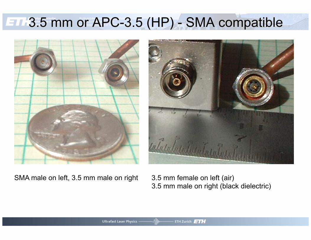
3.5 mm or APC-3.5 (HP) - SMA compatible
SMA male on left, 3.5 mm male on right 3.5 mm female on left (air) 3.5 mm male on right (black dielectric)
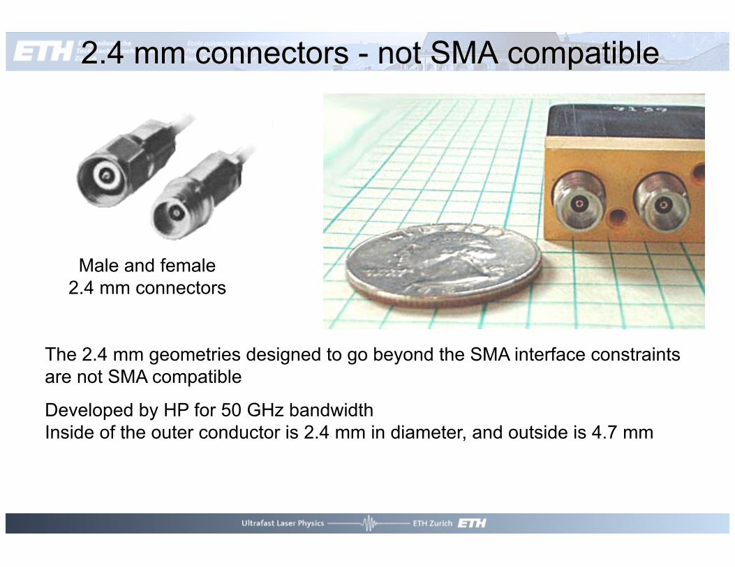
2.4 mm connectors - not SMA compatible
Male and female 2.4 mm connectors
The 2.4 mm geometries designed to go beyond the SMA interface constraints are not SMA compatible
Developed by HP for 50 GHz bandwidth Inside of the outer conductor is 2.4 mm in diameter, and outside is 4.7 mm

Fast photodiode
Rs
J Cp
Equivalent circuit of an ideal photodiode: Ideal current source with a series resistor and a capacitor in parallel
Electrical current generated in photodiode
J =qηPopthν
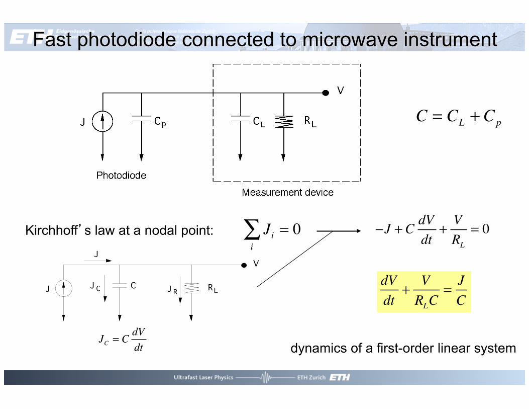
Fast photodiode connected to microwave instrument
Kirchhoff’s law at a nodal point:
Jii∑ = 0
J RL
V
C J RJ C
J
JC = C dVdt
−J + C dVdt
+ VRL
= 0
dVdt
+ VRLC
= JC
dynamics of a first-order linear system
C = CL + Cp

Fast photodiode connected to microwave instrument
dVdt
+ VRLC
= JC
dynamics of a first-order linear system general form in the time domain frequency domain
with the transfer function of the linear system:
τ y + y = xy t( ) = V t( )x t( ) = RLJ t( )τ = RLC = const. τ iω y + y = x
h ω( ) = y
x= 11+ iωτ
C = CL + Cp

Impulse response of microwave test system
3dB bandwidth of measurement system: impulse response (Fourier transform of the transfer function):
h ω( ) = y
x= 11+ iωτ
H ω( ) = h ω( ) 2 = 11+ ωτ( )2
H ω 3dB( ) = 1
2Max H ω( ) ⇒ ω 3dB = 1
τ
h t( ) = 1τe− t /τ ∝ e− t /RLC τ = RLC , f3dB = ω 3dB
2π= 12πRLC

Impulse response of microwave test system
impulse response:
h t( ) = 1τe− t /τ ∝ e− t /RLC
Popt t( )
J t( ) = qηPopt t( )hν
V t( ) = h t( )∗ J t( ) = h t '( ) J t − t '( )∫ dt ' = 1Ce− t '/RLC J t − t '( )∫ dt '
τ = RLC , f3dB = ω 3dB
2π= 12πRLC

Step response of microwave test system
Step response Popt t( )
J t( ) = qηPopt t( )hν
τ = RLC , f3dB = ω 3dB
2π= 12πRLC
V t( ) ∝ 1− e−t τ⎡⎣ ⎤⎦
10% to 90% of the maximum value rise time:
Example: 60 GHz photo detector has a step response of 5.8 ps (i.e. 10%-90% rise time)
Δt ps[ ] = ln9 × τ ps[ ] = 2.2 × τ ps[ ] = 2.2 × 12π f3dB
ps[ ] ≈ 350 GHzf3dB[GHz]
ps[ ]

Gaussian impulse response approximation
impulse response Popt t( )
J t( ) = qηPopt t( )hν
τ = RLC , f3dB = ω 3dB
2π= 12πRLC
h t( ) = exp −t 2 τ 2( )
htot ω( ) = exp − ω2τ1
2
4⎛⎝⎜
⎞⎠⎟exp − ω
2τ 22
4⎛⎝⎜
⎞⎠⎟... = exp −
ω 2 τ12 + τ 2
2 + ...( )4
⎛
⎝⎜
⎞
⎠⎟ = exp − ω
2τ tot2
4⎛⎝⎜
⎞⎠⎟
τ tot = τ12 + τ 2
2 + τ 32 + ... τ FWHM f3dB = 2ln2
π= 0.312
τ FWHM ps[ ] ≈ 312 GHzf3dB[GHz]
ps[ ]p. 6-7, full derivation, example

ideal photodiode:
Electrical current generated in photodiode
Example: GaAs
dielectric constant:
drift velocity:
transit time (should be short): 1 ps
thickness of insulating layer:
Fast photodiode
Rs
J Cp
J =qηPopthν
C = εε0A
d
RL = 50 Ω
ε = 13υs ≈ 10
7 cm / s
d = υsτ trans ≈ 1 µm

ideal photodiode:
Electrical current generated in photodiode
Example: GaAs
dielectric constant:
drift velocity:
transit time (should be short): 1 ps
thickness of insulating layer:
Rs
J Cp
Why do fast photodiodes have a small active area?
C = εε0A
d
RL = 50 Ω
ε = 13υs ≈ 10
7 cm / s
d = υsτ trans ≈ 1 µm
Example: 60 GHz in 50 Ω
τ = RLC , f3dB = ω 3dB
2π= 12πRLC
C ≈ 50 fF
⇒ A ≈ π 12 µm( )2 (r = 12 µm)

Sampling Oscilloscope
Δt
Trigger-Signal für N=1
Δt
N
V(t)
V(t)
Δt(N)1 2 ...

Sampling scope measurement
τtot = τ12+τ22+τ32+...
τFWHM ps⎡
⎣ ⎢ ⎢
⎤
⎦ ⎥ ⎥ ≈ 312 GHz
f3dB [GHz]
0.4ps⎛
⎝ ⎜
⎞
⎠ ⎟
2+ 7.8ps⎛
⎝ ⎜
⎞
⎠ ⎟
2+ 15.6ps⎛
⎝ ⎜ ⎜
⎞
⎠ ⎟ ⎟
2=17.5ps
45.645.545.445.345.245.145.0Sampling timeΔt, ns
laser pulse FWHM ≈ 400 fssampling head: 20 GHzdetector: 40 GHz
19 ps!

Time
Ultrafast Signal Waveform @ f
Sampling Pulses @ f+ Δf
Sampled Waveform @ Δf
Equivalent time sampling

Intensity autocorrelation
I2ω τ( ) ∝ E1 t( )E2 t − τ( ) 2 dt−∞
+∞
∫ E1=E2=E⎯ →⎯⎯⎯ ∝ E t( )E t − τ( ) 2 dt−∞
+∞
∫
I2ω τ( ) ∝ I t( ) I t − τ( )−∞
+∞
∫ dt

Autocorrelation
Nichtlinearer Kristall
λ
λλ/2
• Frequency doubling: blue light intensity depends on the temporal overlap of the two short pulses (in red):
• Delay of the two pulses due to time of flight in a mechanical delay line:
• Signal:
16
0
-40 -20 0 20 40
Verzögerung (fs)
10
Sutter et al.: Spektrum der Wissenschaft,Dossier: Laser (1998)
I2ω Δt( ) = Iω t − Δ t
2( )Iω t + Δ t2( )
−∞
+∞
∫ dt
crystal
Nonlinear crystal
Focusing mirror
Beam splitter
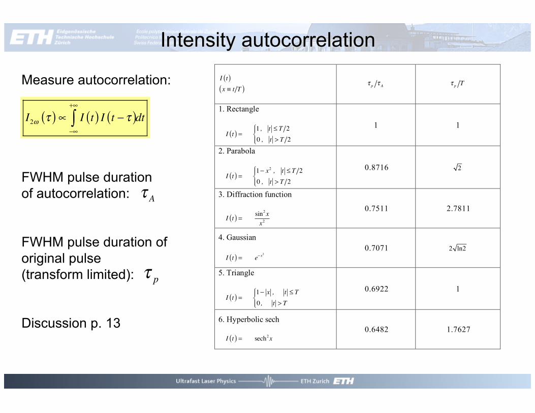
Measure autocorrelation:
FWHM pulse duration of autocorrelation:
FWHM pulse duration of original pulse (transform limited):
Discussion p. 13
Intensity autocorrelation
I2ω τ( ) ∝ I t( ) I t − τ( )−∞
+∞
∫ dt
I t( ) x ≡ t T( )
τ p τ A τ p T
1. Rectangle
I t( ) = 1 , t ≤ T 20 , t > T 2
⎧⎨⎪
⎩⎪
1 1
2. Parabola
I t( ) = 1− x2 , t ≤ T 2
0 , t > T 2
⎧⎨⎪
⎩⎪
0.8716 2
3. Diffraction function
I t( ) = sin2xx2
0.7511 2.7811
4. Gaussian I t( ) = e− x2
0.7071 2 ln2
5. Triangle
I t( ) = 1− x , t ≤ T0, t > T
⎧⎨⎪
⎩⎪
0.6922 1
6. Hyperbolic sech I t( ) = sech2x
0.6482 1.7627
τ A
τ p

Translation stage:
True time shift of one of the pulse:
Measured time shift of autocorrelation signal on oscilloscope:
Time calibration:
Calibration of intensity autocorrelation
I2ω τ( ) ∝ I t( ) I t − τ( )−∞
+∞
∫ dt
Δz0
Δttrue =2Δz0c
Δz0
Δttrue ⇔ ΔτΔτ
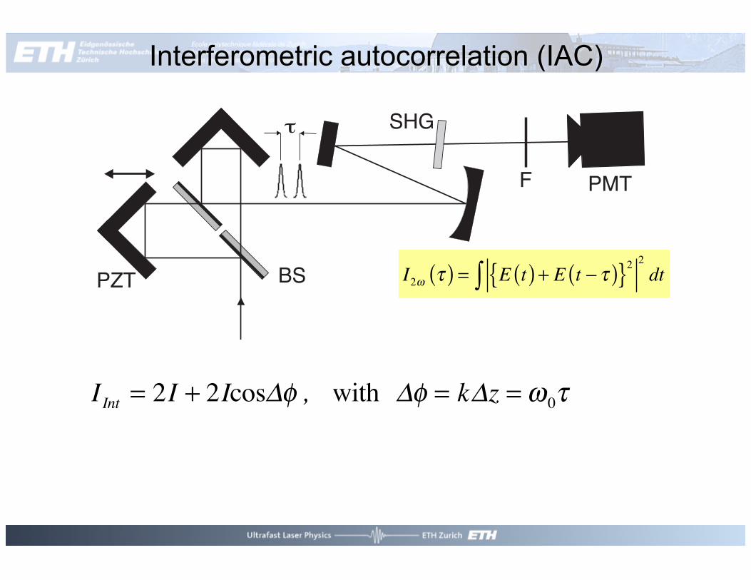
Interferometric autocorrelation (IAC)
IInt = 2I + 2IcosΔφ , with Δφ = kΔz = ω0τ
I2ω τ( ) = E t( ) + E t − τ( ) 22dt∫
Appl. Phys. B 65, 175 (‘97)
Appl. Phys. B 65, 189 (‘97)
Appl. Phys. Lett. 74, 2268 (‘99)
Opt. Lett. 24, 631 (‘99)
8
6
4
2
0
IAC
(a.u
.)
-20 -10 0 10 20
Delay (fs)
8
6
4
2
0
-20 -10 0 10 20
A B
C D
OPA COMP.I
COMP.II LASER
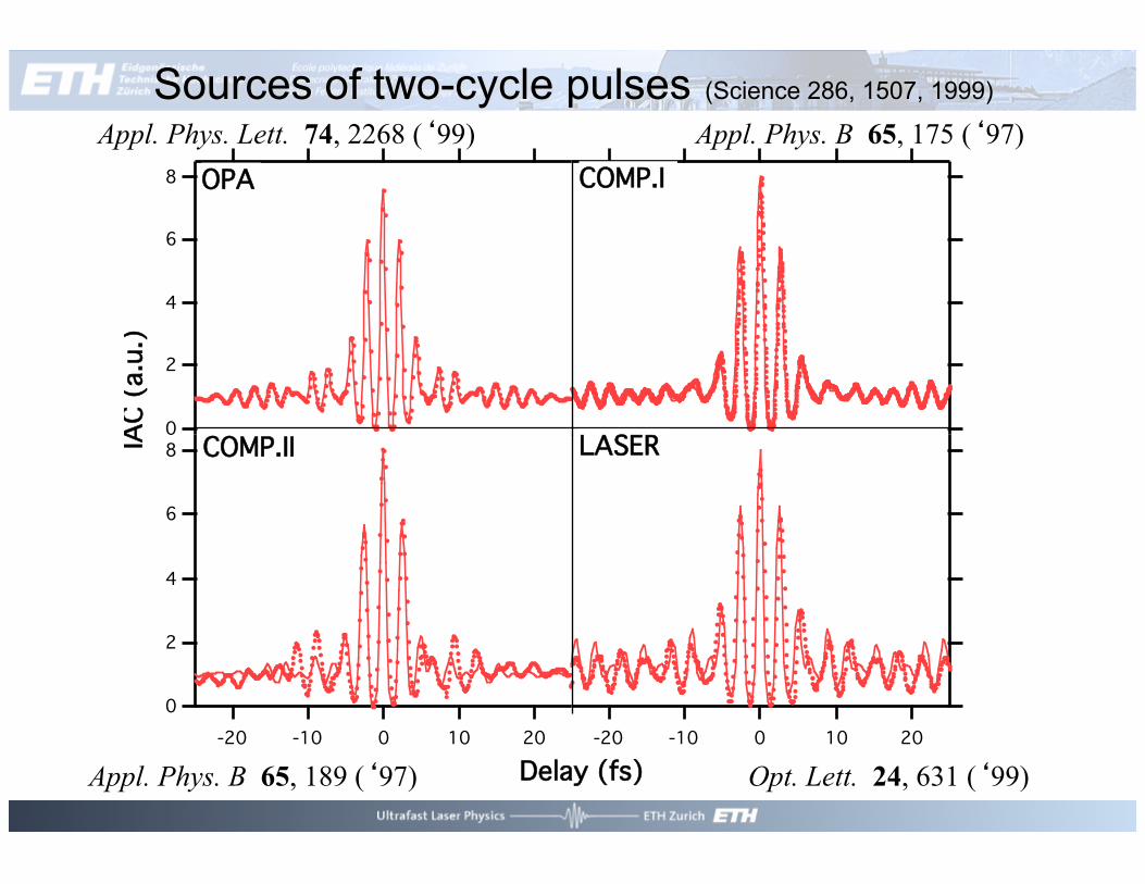
Sources of two-cycle pulses (Science 286, 1507, 1999)

Nonlinear interaction is required for pulse measurement
Without nonlinear interaction we measure interferogram of fundamental pulse:
Fourier transform of this interferogram gives the optical intensity spectrum:
(Fourier spectrography)
I τ( ) =E t( ) + E t − τ( )∫
2dt
2 E t( ) 2 dt∫= 1+
E∗ t( )E t − τ( ) + E t( )E∗ t − τ( )⎡⎣ ⎤⎦∫ dt
2 E t( ) 2 dt∫
F I τ( ) = F 1 +E∗ −ω( ) E −ω( ) + E ω( ) E∗ ω( )
2 E t( ) 2 dt∫= F 1 + I −ω( ) + I ω( )
2 E t( ) 2 dt∫
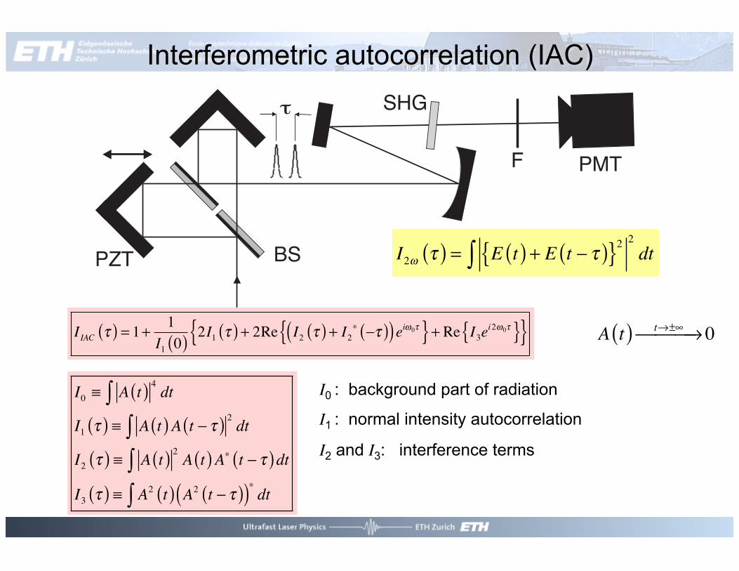
Interferometric autocorrelation (IAC)
I2ω τ( ) = E t( ) + E t − τ( ) 22dt∫
I0 ≡ A t( ) 4 dt∫I1 τ( ) ≡ A t( )A t − τ( ) 2 dt∫I2 τ( ) ≡ A t( ) 2 A t( )A∗ t − τ( )dt∫I3 τ( ) ≡ A2 t( )∫ A2 t − τ( )( )∗ dt
IIAC τ( ) = 1+ 1I1 0( ) 2I1 τ( ) + 2Re I2 τ( ) + I2∗ −τ( )( )eiω0τ + Re I3e
i2ω0τ A t( ) t→±∞⎯ →⎯⎯ 0
I0 : background part of radiation
I1 : normal intensity autocorrelation
I2 and I3: interference terms

Interferometric autocorrelation (IAC)
8
6
4
2
0
-60 -40 -20 0 20 40 60Time [fs]
Calculation:
10 fs sech2-pulse
Measurement:
Modelocked Ti:sapphire laser
8
6
4
2
0
Inte
nsity
[a.u
.]
-40 -20 0 20 40Time delay o [fs]
ideal 10 fs sech2
experimental

Interferometric autocorrelation (IAC) 8
6
4
2
0
-60 -40 -20 0 20 40 60Time [fs]
IIAC τ( ) = IIAC −τ( )
IIAC τ → ±∞( ) = 1IIAC τ( )
max= IIAC 0( ) = 8
IIAC τ( )min
= 0
Non-background free intensity autocorrelation I2ωcollinear τ = 0( )
I2ωcollinear τ → ∞( ) =
31

IAC provides some information about chirped pulses 8
6
4
2
0
-80 -60 -40 -20 0 20 40 60 80Time [fs]
GDD = 50 fs2
8
6
4
2
0
-80 -60 -40 -20 0 20 40 60 80Time [fs]
GDD = 100 fs2
8
6
4
2
0
-80 -60 -40 -20 0 20 40 60 80Time [fs]
GDD = 200 fs2
Δν > ΔνTB
⇒ τ coh =1Δν
< 1ΔνTB
≈ τ p
⇒ τ coh <τ p
TB: time bandwidth limited
coh: coherence time
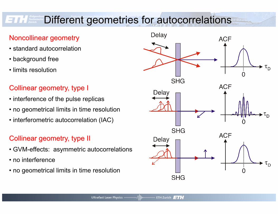
Different geometries for autocorrelations Noncollinear geometry • standard autocorrelation
• background free
• limits resolution
Collinear geometry, type I • interference of the pulse replicas
• no geometrical limits in time resolution
• interferometric autocorrelation (IAC)
Collinear geometry, type II • GVM-effects: asymmetric autocorrelations
• no interference
• no geometrical limits in time resolution

Temporal resolution in noncollinear setups
θ
0−τ +τ
x
z
ωω
2ω
0
δt = θ0w0c
τm2 = τ p
2 +δt2
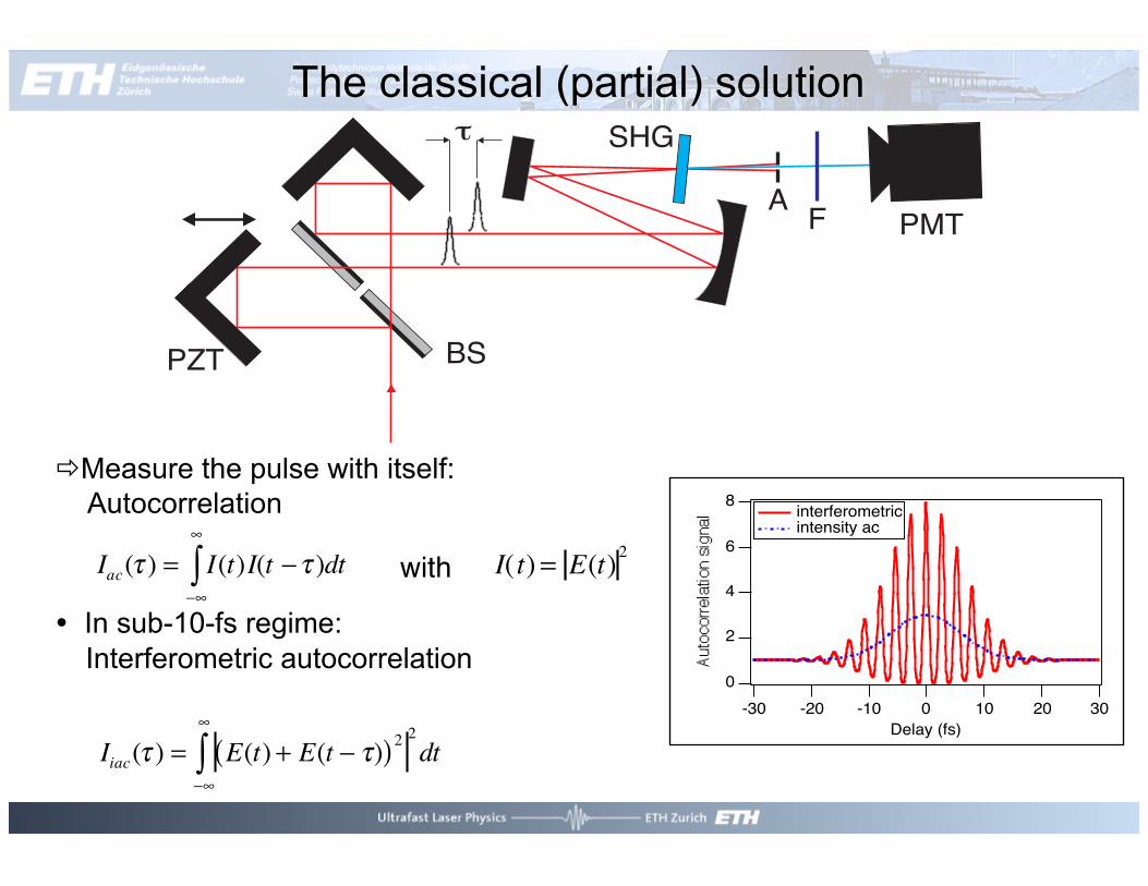
The classical (partial) solution
Measure the pulse with itself: Autocorrelation
In sub-10-fs regime: Interferometric autocorrelation
Iac(τ ) = I(t)I(t −τ )dt−∞
∞
∫ I( t) = E(t)2with!
Iiac(τ ) = E(t) + E(t − τ)( )22dt
−∞
∞
∫
8
6
4
2
0-30 -20 -10 0 10 20 30
Delay (fs)
interferometric intensity ac
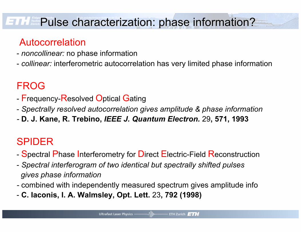
Pulse characterization: phase information? Autocorrelation - noncollinear: no phase information - collinear: interferometric autocorrelation has very limited phase information FROG - Frequency-Resolved Optical Gating - Spectrally resolved autocorrelation gives amplitude & phase information - D. J. Kane, R. Trebino, IEEE J. Quantum Electron. 29, 571, 1993 SPIDER - Spectral Phase Interferometry for Direct Electric-Field Reconstruction - Spectral interferogram of two identical but spectrally shifted pulses gives phase information - combined with independently measured spectrum gives amplitude info - C. Iaconis, I. A. Walmsley, Opt. Lett. 23, 792 (1998)
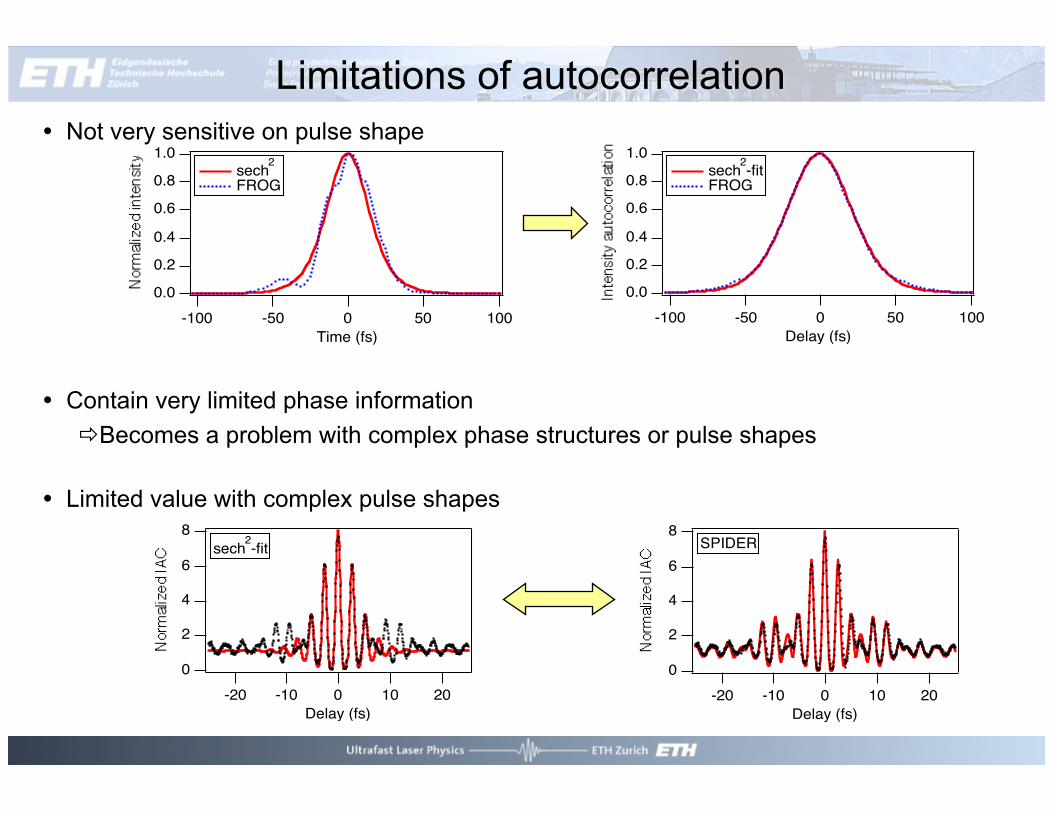
Limitations of autocorrelation Not very sensitive on pulse shape
Contain very limited phase information Becomes a problem with complex phase structures or pulse shapes
Limited value with complex pulse shapes
8
6
4
2
0
-20 -10 0 10 20Delay (fs)
SPIDER8
6
4
2
0
-20 -10 0 10 20Delay (fs)
sech2-fit
1.0
0.8
0.6
0.4
0.2
0.0-100 -50 0 50 100
Time (fs)
sech2
FROG
1.0
0.8
0.6
0.4
0.2
0.0-100 -50 0 50 100
Delay (fs)
sech2-fit FROG

FROG
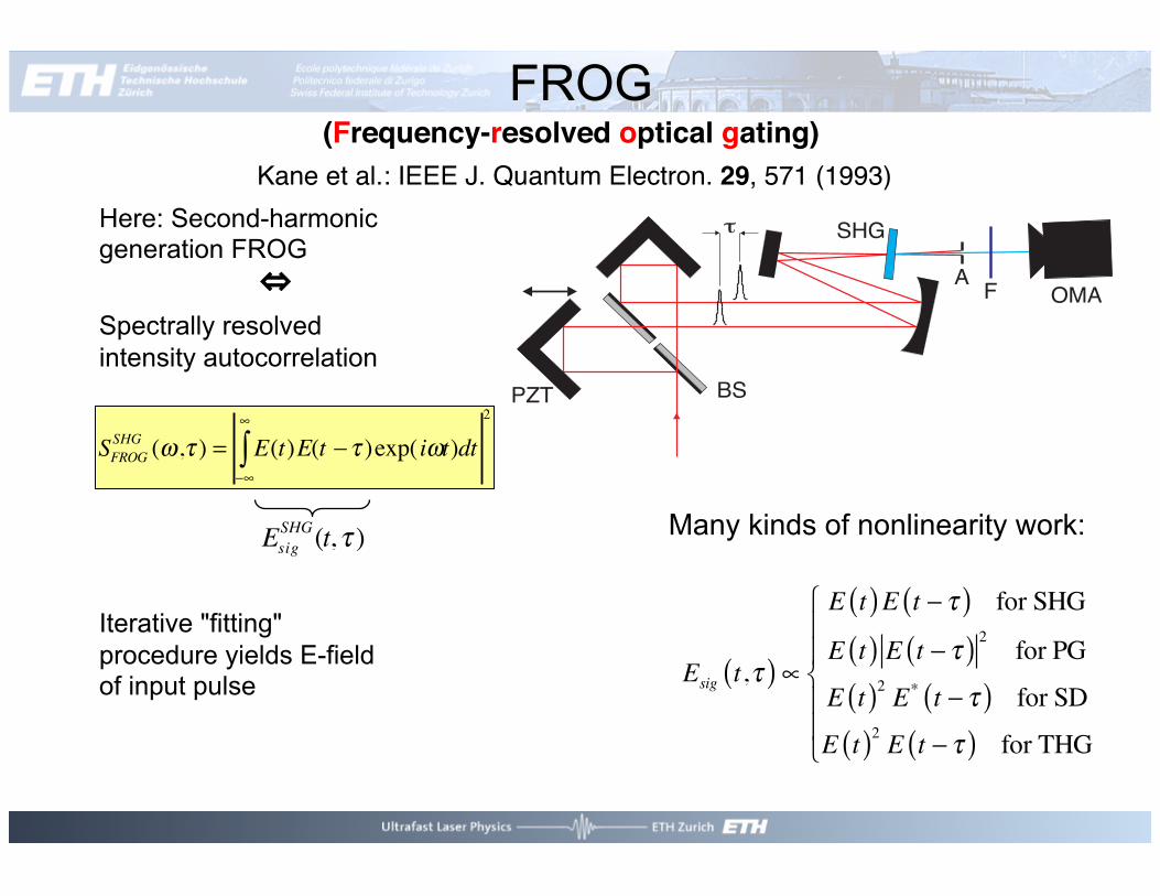
Here: Second-harmonic generation FROG Spectrally resolved intensity autocorrelation Iterative "fitting" procedure yields E-field of input pulse
(Frequency-resolved optical gating)!Kane et al.: IEEE J. Quantum Electron. 29, 571 (1993)"
⇔!
Knowledge ofsignal generation
process!
Measured data!
SFROGSHG (ω,τ ) = E(t)E(t −τ )
−∞
∞
∫ exp( iωt)dt2
EsigSHG(t, τ )
FROG
Here: Second-harmonic generation FROG Spectrally resolved intensity autocorrelation Iterative "fitting" procedure yields E-field of input pulse
(Frequency-resolved optical gating)!Kane et al.: IEEE J. Quantum Electron. 29, 571 (1993)"
⇔!
SFROGSHG (ω,τ ) = E(t)E(t −τ )
−∞
∞
∫ exp( iωt)dt2
EsigSHG(t, τ )
Esig t,τ( ) ∝
E t( )E t − τ( ) for SHG
E t( ) E t − τ( ) 2 for PG
E t( )2 E* t − τ( ) for SD
E t( )2 E t − τ( ) for THG
⎧
⎨
⎪⎪
⎩
⎪⎪
Many kinds of nonlinearity work:

PG-FROG
Polarization gating (PG): polarizers are oriented at 0° and 90° an intense 45°-polarized beam (at frequency w2) induces birefringence and therefore a polarization rotation of the 0°-polarized beam (at frequency w1), which can then leak through the second 90° polarizer. The pulse at the output indicates the signal pulse, again collinear with one of the input beams, but here with the orthogonal polarization.
R. Trebino, Kluwer Academic Publishers, Boston, 2002, ISBN 1-4020-7066-7
Esig t,τ( ) ∝E t( )E t − τ( ) for SHG
E t( ) E t − τ( ) 2 for PG
⎧⎨⎪
⎩⎪
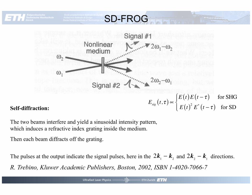
SD-FROG
Self-diffraction: The two beams interfere and yield a sinusoidal intensity pattern, which induces a refractive index grating inside the medium.
Then each beam diffracts off the grating.
The pulses at the output indicate the signal pulses, here in the and directions.
R. Trebino, Kluwer Academic Publishers, Boston, 2002, ISBN 1-4020-7066-7
Esig t,τ( ) ∝E t( )E t − τ( ) for SHG
E t( )2 E* t − τ( ) for SD
⎧⎨⎪
⎩⎪
2k1 − k2 2k2 − k1

THG-FROG
Third harmonic generation:
While each beam individually can produce third harmonic, it can also be produced by two factors of one field and one of the other.
These latter two cases are shown here.
R. Trebino, Kluwer Academic Publishers, Boston, 2002, ISBN 1-4020-7066-7
Esig t,τ( ) ∝E t( )E t − τ( ) for SHG
E t( )2 E t − τ( ) for THG
⎧⎨⎪
⎩⎪

FROG
R. Trebino, Kluwer Academic Publishers, Boston, 2002, ISBN 1-4020-7066-7
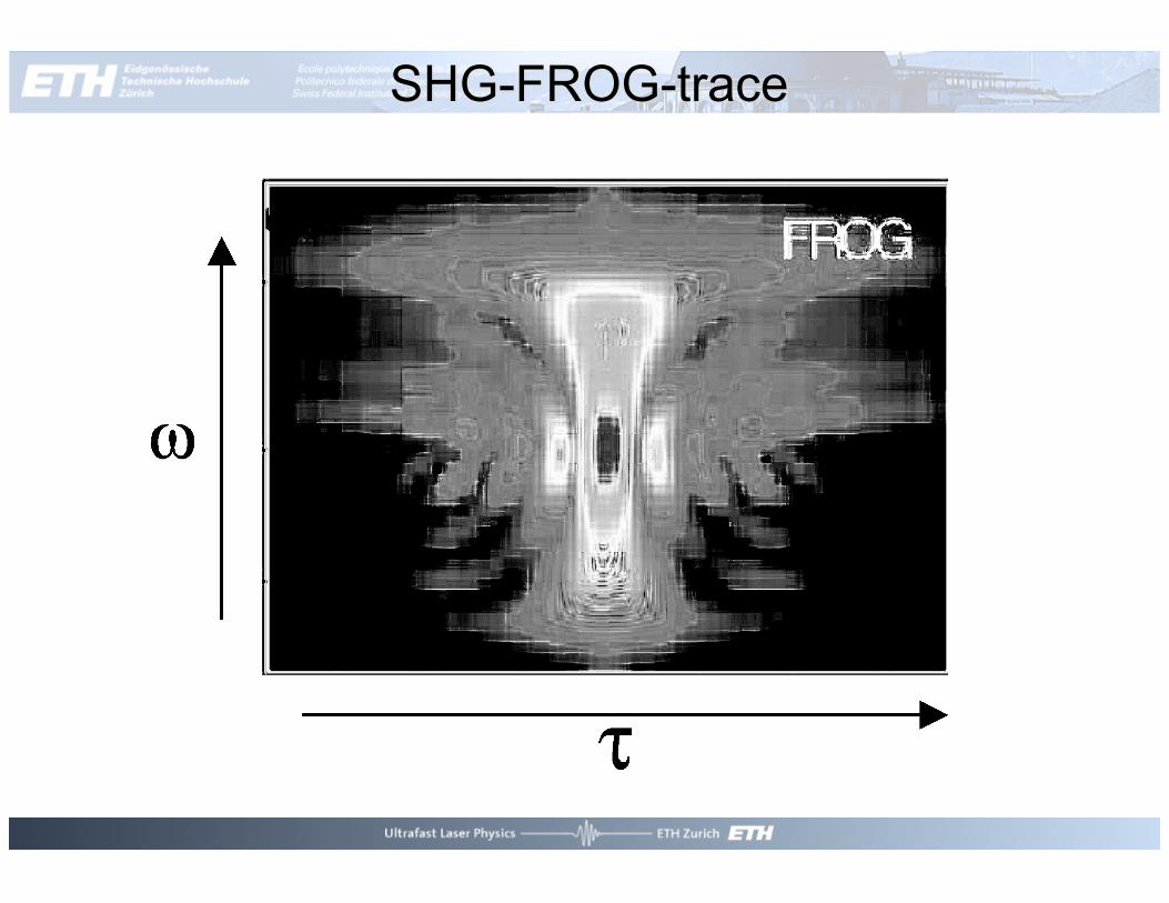
SHG-FROG-trace

FROG

FROG projections algorithm
E ω ,τ( ) = F Esig t,τ( ) = Esig t,τ( )∫ exp −iωt( )dt
IFROG ω ,τ( ) = Esig t,τ( )exp −iωt( )dt∫2
IFROG ω ,τ( )eiφ ω ,τ( ) = Esig t,τ( )exp −iωt( )dt∫

Measurement of pulses in the two-cycle regime
transform limit: 5.3 fs sech2-fit: 4.5 fs!!
8
6
4
2
0
Norm
alize
d IA
C
-60 -40 -20 0 20 40 60Delay (fs)
calculated measured
1.0
0.8
0.6
0.4
0.2
0.0
Norm
alize
d in
tens
ity
-60 -40 -20 0 20 40 60Time (fs)
-60 -40 -20 0 20 40 60Delay (fs)
5.5
5.0
4.5
4.0
Angu
lar f
requ
ency
(fs
-1)
Measured
-60 -40 -20 0 20 40 60Delay (fs)
5.5
5.0
4.5
4.0
Angu
lar f
requ
ency
(fs
-1)
Reconstructed
tFWHM = 6.6 fs

FROG vs SPIDER
SPIDER!
FROG!
SPIDER: Straightforward to extend to significantly shorter pulses !
FROG: One setup may cover a large range of pulse durations!

Interpretation of the spectral phase ϕ(ω)
ϕ (ω ) =ϕ0 +dϕdω ω0
ω − ω0( ) + 12d 2ϕdω 2
ω 0
(ω − ω0 )2 + 1
6d 3ϕdω 3
ω 0
(ω −ω 0 )3 + ...
3.0
2.8
2.6
2.42.2
2.0
1.8
-40 0 40Time (fs)
Transform limited3.0
2.8
2.6
2.4
2.2
2.0
1.8
-40 0 40Time (fs)
GDD = 50 fs23.0
2.8
2.6
2.42.2
2.0
1.8
-40 0 40Time (fs)
TOD = 500 fs3
The spectral phase rearranges the frequency components in the temporal domain!
Linear chirp! Nonlinear chirp!Transform limited(shortest possible pulse)!
Chirp!

SPIDER (Spectral phase interferometry for direct electric-field reconstruction)!
Iaconis et al.: Opt. Lett. 23, 792 (1998)" Gallmann et al.: Opt. Lett. 24, 1314 (1999)"
T >> τ >> τp(3 ps >> 300 fs >> 6 fs)!
SFG"
3.0
2.8
2.6
2.4
2.2
2.0
1.8
-1500 -1000 -500 0 500 1000 1500Time (fs)
τ
δω
1.0
0.8
0.6
0.4
0.2
0.0
5.25.04.84.64.44.2Frequency (fs-1)
δω
S(ω ) = E(ω )2 + E(ω +δω )2 + 2E(ω )E(ω + δω) cos ϕ(ω +δω ) −ϕ (ω ) +ωτ( )

OMA
GDD
Δt
PRBS
SPIDER
Slow variations in conversion efficiency over the pulse spectrum do not influence the reconstructed spectral phase!
τ
ω+δω" ω"
BBO-crystal!
Iaconis et al.: Opt. Lett. 23, 792 (1998)" Gallmann et al.: Opt. Lett. 24, 1314 (1999)"
1.0
0.5
0.0
Inte
rfer
ogra
m
460400340Wavelength (nm)
Only phase term - No amplitude information used!!!φ(ω) from SPIDER + independently measured pulse spectrum!+ Fourier transformation results in E(t) and P(t)!
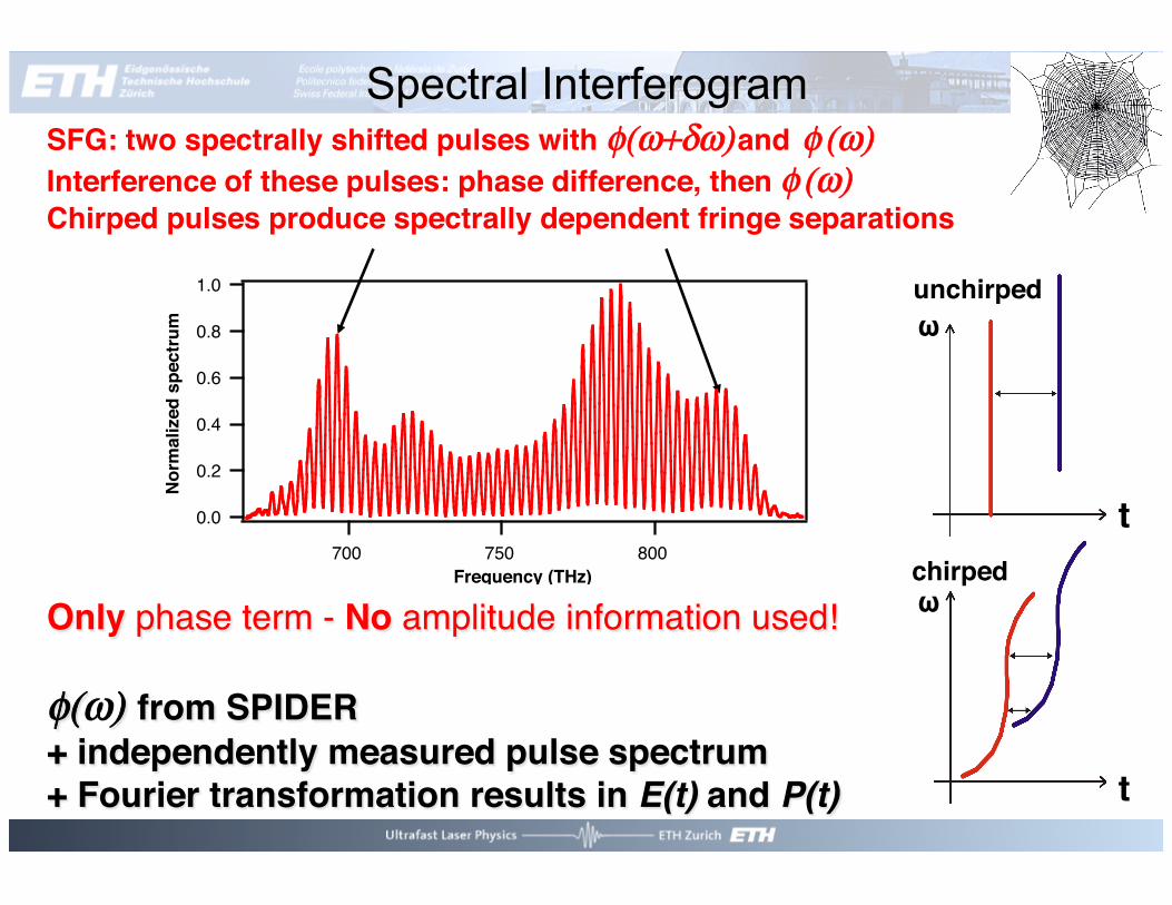
Spectral Interferogram SFG: two spectrally shifted pulses with φ(ω+δω) and φ (ω) !Interference of these pulses: phase difference, then φ (ω) !Chirped pulses produce spectrally dependent fringe separations!
"
1.0
0.8
0.6
0.4
0.2
0.0
Nor
mal
ized
spe
ctru
m
800750700Frequency (THz)
ω!
t!
ω!
unchirped!
chirped!
t!

Phase extraction in SPIDER S ω( ) = E ω( ) 2 + E ω + δω( ) 2 + 2 E ω( )E ω + δω( ) cos ϕ ω + δω( ) −ϕ ω( ) +ωτ( )
1.0
0.8
0.6
0.4
0.2
0.0
5.25.04.84.64.44.2Frequency (fs-1)
δω
A
C* C
g ω( ) = a ω( ) + b ω( )cos φ ω( ) +ωτ( )
g ω( ) = a ω( ) + c ω( )eiωτ + c* ω( )e− iωτ ,
with c ω( ):= 12b ω( )eiφ ω( )
FFT ⇒ G t( ) = A t( ) + C t − τ( ) + C* t + τ( )
IFFT of C t − τ( ) ⇒ c ω( )eiωτ
Im log c ω( )eiωτ⎡⎣ ⎤⎦ = Im log 12 b ω( )⎡⎣ ⎤⎦ + i φ ω( ) +ωτ⎡⎣ ⎤⎦ = φ ω( ) +ωτ
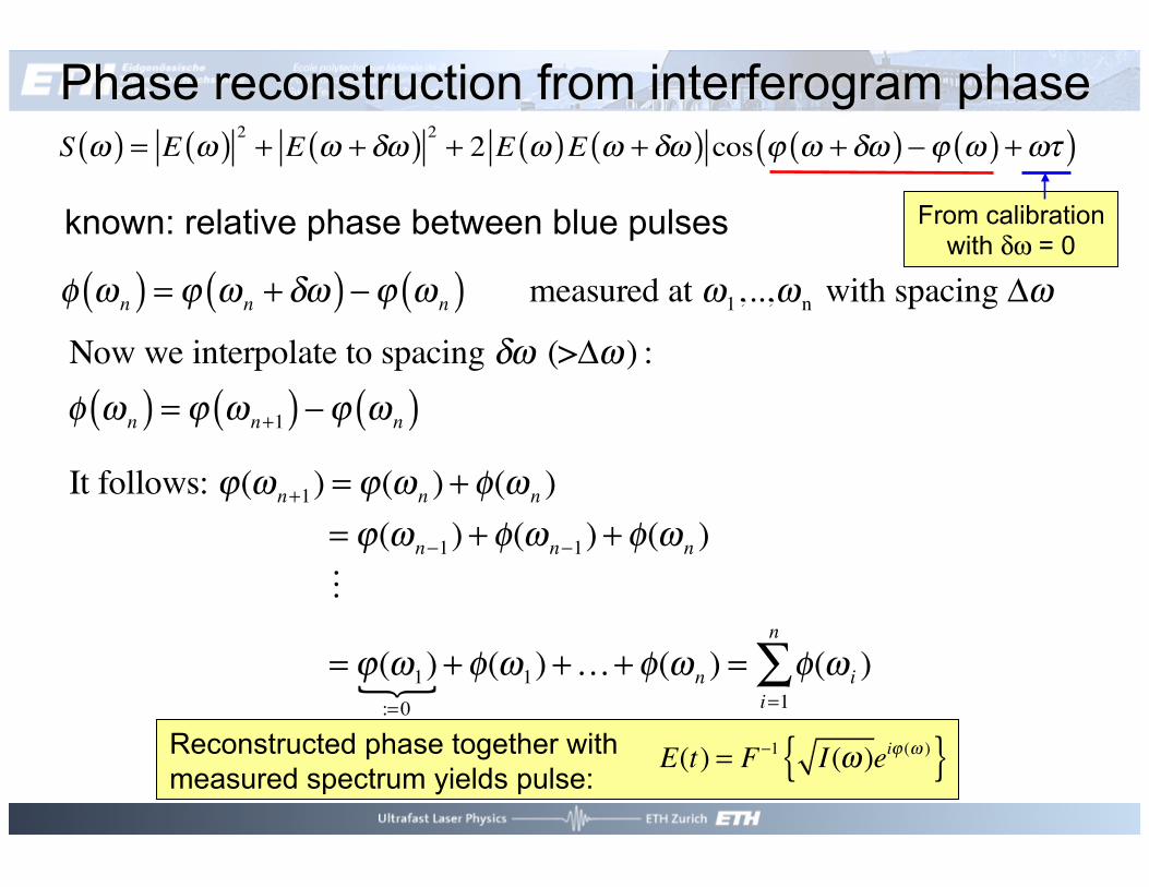
S ω( ) = E ω( ) 2 + E ω + δω( ) 2 + 2 E ω( )E ω + δω( ) cos ϕ ω + δω( ) −ϕ ω( ) +ωτ( )Phase reconstruction from interferogram phase
known: relative phase between blue pulses
φ ωn( ) = ϕ ωn + δω( ) −ϕ ωn( ) measured at ω1,..,ωn with spacing Δω
Now we interpolate to spacing δω (>Δω ) : φ ωn( ) = ϕ ωn+1( ) −ϕ ωn( )
It follows: ϕ(ωn+1) = ϕ(ωn ) + φ(ωn ) = ϕ(ωn−1) + φ(ωn−1) + φ(ωn )
= ϕ(ω1):=0 + φ(ω1) +…+ φ(ωn ) = φ(ω i )
i=1
n
∑Reconstructed phase together with measured spectrum yields pulse:
E(t) = F−1 I(ω )eiϕ (ω )
From calibration with δω = 0

Measurement of pulses in the two-cycle regime
transform limit: 5.3 fs
1.0
0.8
0.6
0.4
0.2
0.0Norm
alize
d sp
ectru
m
440420400380360Wavelength (nm)
tFWHM = 5.9 fs
3.0
2.8
2.6
2.4
2.2
2.0
150100500-50-100Time (fs)
1.0
0.8
0.6
0.4
0.2
0.0
1000900800700600Wavelength (nm)
-1.5
-1.0
-0.5
0.0
0.5
1.0
1.5
1.0
0.8
0.6
0.4
0.2
0.0-60 -40 -20 0 20 40 60
Time (fs)
D. H. Sutter, et al., Opt. Lett. 24, 631, 1999 and Appl. Phys. B 70, S5, 2000
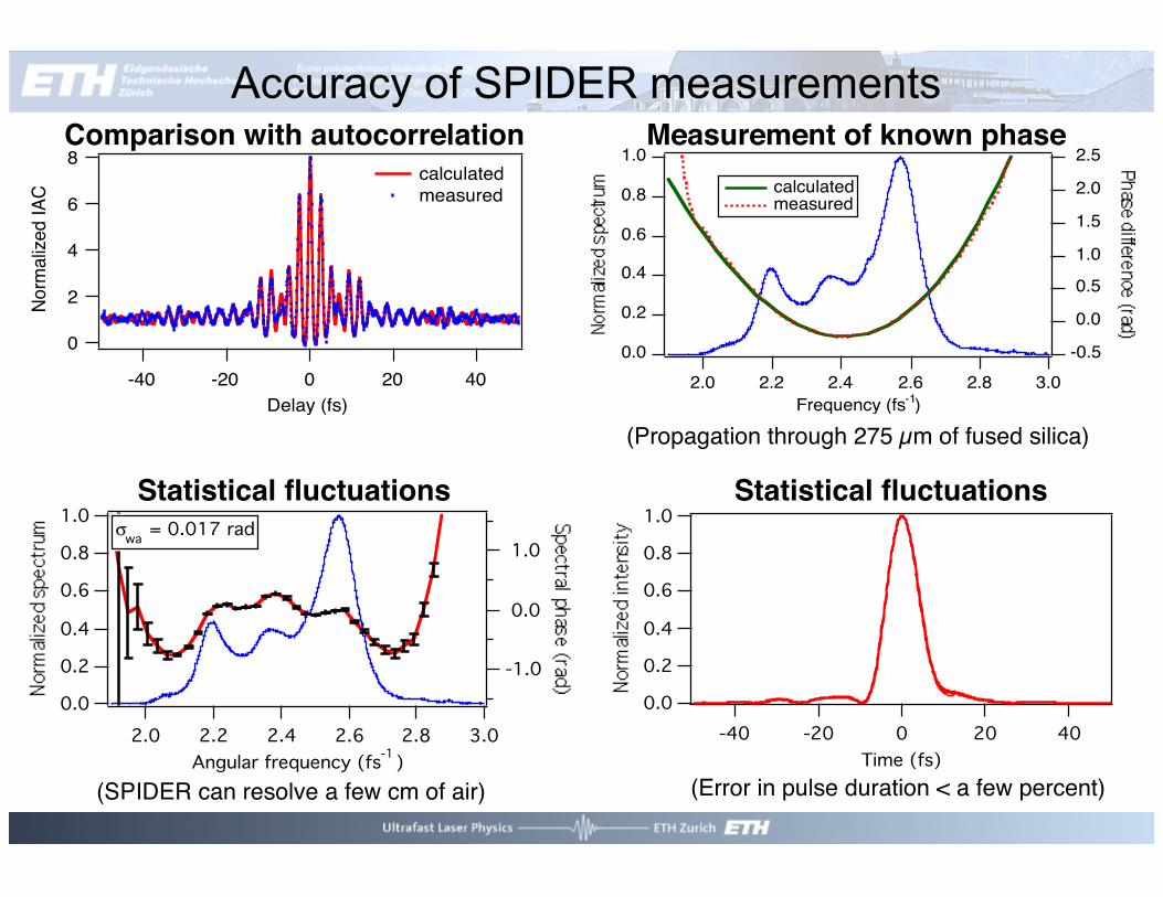
Accuracy of SPIDER measurements 8
6
4
2
0
Norm
alize
d IA
C
-40 -20 0 20 40Delay (fs)
calculated measured
1.0
0.8
0.6
0.4
0.2
0.03.02.82.62.42.22.0
Angular frequency (fs-1)
-1.0
0.0
1.0σwa = 0.017 rad 1.0
0.8
0.6
0.4
0.2
0.0-40 -20 0 20 40
Time (fs)
1.0
0.8
0.6
0.4
0.2
0.0
3.02.82.62.42.22.0Frequency (fs-1)
2.5
2.0
1.5
1.0
0.5
0.0
-0.5
calculated measured
Comparison with autocorrelation!
Statistical fluctuations! Statistical fluctuations!
Measurement of known phase!
(Propagation through 275 µm of fused silica)"
(Error in pulse duration < a few percent)"(SPIDER can resolve a few cm of air)"

Need amplitude & phase measurements
Sub-10-fs Ti:sapphire laser: Measured IAC (dotted line) Measured SPIDER - calculated IAC trace (solid line) very good agreement - SPIDER: 5.9 fs FWHM Ideal sech2-fit to IAC (solid line) - no good in the wings! - ideal sech2-fit: 4.5 fs FWHM Measured optical spectrum - transform-limit: 5.3 fs FWHM Other fits to IAC trace - generally underestimating FWHM
8
6
4
2
0-20 -10 0 10 20
Delay (fs)
sech2-fitτ = 4.5 fs
8
6
4
2
0
SPIDERτ = 5.9 fs
Appl. Phys. B 70, S67, 2000 L. Gallmann et al.Techniques for characterization of sub-10-fs pulses: a comparison"
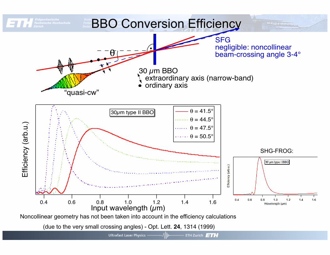
BBO Conversion Efficiency
Noncollinear geometry has not been taken into account in the efficiency calculations
(due to the very small crossing angles) - Opt. Lett. 24, 1314 (1999)
Effic
ienc
y (a
rb.u
.)
1.61.41.21.00.80.60.4Input wavelength (µm)
θ = 41.5° θ = 44.5° θ = 47.5° θ = 50.5°
30µm type II BBO
30 µm BBO extraordinary axis (narrow-band) ordinary axis
θSFGnegligible: noncollinear beam-crossing angle 3-4°
“quasi-cw”
SHG-FROG: