88rds37/teaching/statistical...88 Paper 4, Section I 5K Statistical Modelling Consider the normal...

88

Paper 4, Section I

5K Statistical ModellingConsider the normal linear model where the n-vector of responses Y satisfies

Y = Xβ + ε with ε ∼ Nn(0, σ2I) and X is an n × p design matrix with full column

rank. Write down a (1− α)-level confidence set for β.

Define the Cook’s distance for the observation (Yi, xi) where xTi is the ith row of X,

and give its interpretation in terms of confidence sets for β.

In the model above with n = 100 and p = 4, you observe that one observation hasCook’s distance 3.1. Would you be concerned about the influence of this observation?Justify your answer.

[Hint: You may find some of the following facts useful:

1. If Z ∼ χ24, then P(Z 6 1.06) = 0.1, P(Z 6 7.78) = 0.9.

2. If Z ∼ F4,96, then P(Z 6 0.26) = 0.1, P(Z 6 2.00) = 0.9.

3. If Z ∼ F96,4, then P(Z 6 0.50) = 0.1, P(Z 6 3.78) = 0.9.]

Part II, 2014 List of Questions

89

Paper 3, Section I

5K Statistical ModellingIn an experiment to study factors affecting the production of the plastic polyvinyl

chloride (PVC), three experimenters each used eight devices to produce the PVC andmeasured the sizes of the particles produced. For each of the 24 combinations of deviceand experimenter, two size measurements were obtained.

The experimenters and devices used for each of the 48 measurements are stored inR as factors in the objects experimenter and device respectively, with the measurementsthemselves stored in the vector psize. The following analysis was performed in R.

> fit0 <- lm(psize ~ experimenter + device)

> fit <- lm(psize ~ experimenter + device + experimenter:device)

> anova(fit0, fit)

Analysis of Variance Table

Model 1: psize ~ experimenter + device

Model 2: psize ~ experimenter + device + experimenter:device

Res.Df RSS Df Sum of Sq F Pr(>F)

1 38 49.815

2 24 35.480 14 14.335 0.6926 0.7599

Let X and X0 denote the design matrices obtained by model.matrix(fit) andmodel.matrix(fit0) respectively, and let Y denote the response psize. Let P and P0

denote orthogonal projections onto the column spaces of X and X0 respectively.

For each of the following quantities, write down their numerical values if they appearin the analysis of variance table above; otherwise write ‘unknown’.

1. ‖(I − P )Y ‖2

2. ‖X(XTX)−1XTY ‖2

3. ‖(I − P0)Y ‖2 − ‖(I − P )Y ‖2

4.‖(P − P0)Y ‖2/14‖(I − P )Y ‖2/24

5.∑48

i=1 Yi/48

Out of the two models that have been fitted, which appears to be the moreappropriate for the data according to the analysis performed, and why?

Part II, 2014 List of Questions [TURN OVER

90

Paper 2, Section I

5K Statistical ModellingDefine the concept of an exponential dispersion family. Show that the family of

scaled binomial distributions 1nBin(n, p), with p ∈ (0, 1) and n ∈ N, is of exponential

dispersion family form.

Deduce the mean of the scaled binomial distribution from the exponential dispersionfamily form.

What is the canonical link function in this case?

Paper 1, Section I

5K Statistical ModellingWrite down the model being fitted by the following R command, where y ∈ 0, 1, 2, . . .n

and X is an n× p matrix with real-valued entries.

fit <- glm(y ~ X, family = poisson)

Write down the log-likelihood for the model. Explain why the command

sum(y) - sum(predict(fit, type = "response"))

gives the answer 0, by arguing based on the log-likelihood you have written down.[Hint: Recall that if Z ∼ Pois(µ) then

P(Z = k) =µke−µ

k!

for k ∈ 0, 1, 2, . . ..]


91

Paper 4, Section II

13K Statistical ModellingIn a study on infant respiratory disease, data are collected on a sample of 2074

infants. The information collected includes whether or not each infant developed arespiratory disease in the first year of their life; the gender of each infant; and detailson how they were fed as one of three categories (breast-fed, bottle-fed and supplement).The data are tabulated in R as follows:

disease nondisease gender food

1 77 381 Boy Bottle-fed

2 19 128 Boy Supplement

3 47 447 Boy Breast-fed

4 48 336 Girl Bottle-fed

5 16 111 Girl Supplement

6 31 433 Girl Breast-fed

Write down the model being fit by the R commands on the following page:


92

> total <- disease + nondisease

> fit <- glm(disease/total ~ gender + food, family = binomial,

+ weights = total)

The following (slightly abbreviated) output from R is obtained.

> summary(fit)

Coefficients:

Estimate Std. Error z value Pr(>|z|)

(Intercept) -1.6127 0.1124 -14.347 < 2e-16 ***

genderGirl -0.3126 0.1410 -2.216 0.0267 *

foodBreast-fed -0.6693 0.1530 -4.374 1.22e-05 ***

foodSupplement -0.1725 0.2056 -0.839 0.4013

---

Signif. codes: 0 *** 0.001 ** 0.01 * 0.05 . 0.1 1

(Dispersion parameter for binomial family taken to be 1)

Null deviance: 26.37529 on 5 degrees of freedom

Residual deviance: 0.72192 on 2 degrees of freedom

Briefly explain the justification for the standard errors presented in the output above.

Explain the relevance of the output of the following R code to the data being studied,justifying your answer:

> exp(c(-0.6693 - 1.96*0.153, -0.6693 + 1.96*0.153))

[1] 0.3793940 0.6911351

[Hint: It may help to recall that if Z ∼ N(0, 1) then P(Z > 1.96) = 0.025.]

Let D1 be the deviance of the model fitted by the following R command.

> fit1 <- glm(disease/total ~ gender + food + gender:food,

+ family = binomial, weights = total)

What is the numerical value of D1? Which of the two models that have been fitted shouldyou prefer, and why?


93

Paper 1, Section II

13K Statistical ModellingConsider the normal linear model where the n-vector of responses Y satisfies

Y = Xβ + ε with ε ∼ Nn(0, σ2I). Here X is an n × p matrix of predictors with full

column rank where n > p+ 3, and β ∈ Rp is an unknown vector of regression coefficients.Let X0 be the matrix formed from the first p0 < p columns of X, and partition β asβ = (βT

0 , βT1 )

T where β0 ∈ Rp0 and β1 ∈ Rp−p0. Denote the orthogonal projections ontothe column spaces of X and X0 by P and P0 respectively.

It is desired to test the null hypothesisH0 : β1 = 0 against the alternative hypothesisH1 : β1 6= 0. Recall that the F -test for testing H0 against H1 rejects H0 for large valuesof

F =‖(P − P0)Y ‖2/(p − p0)

‖(I − P )Y ‖2/(n − p).

Show that (I − P )(P − P0) = 0, and hence prove that the numerator and denominator ofF are independent under either hypothesis.

Show that

Eβ,σ2(F ) =(n − p)(τ2 + 1)

n− p− 2,

where τ2 =‖(P − P0)Xβ‖2

(p− p0)σ2.

[In this question you may use the following facts without proof: P − P0 is an or-thogonal projection with rank p − p0; any n × n orthogonal projection matrix Π satisfies‖Πε‖2 ∼ σ2χ2

ν , where ν = rank(Π); and if Z ∼ χ2ν then E(Z−1) = (ν − 2)−1 when ν > 2.]


88

Paper 4, Section I

5J Statistical ModellingThe output X of a process depends on the levels of two adjustable variables: A, a

factor with four levels, and B, a factor with two levels. For each combination of a level ofA and a level of B, nine independent values of X are observed.

Explain and interpret the R commands and (abbreviated) output below. Inparticular, describe the model being fitted, and describe and comment on the hypothesistests performed under the summary and anova commands.

> fit1 <- lm(x ˜ a+b)

> summary(fit1)

Coefficients:

Estimate Std. Error t value Pr(>|t|)

(Intercept) 2.5445 0.2449 10.39 6.66e-16 ***

a2 -5.6704 0.4859 -11.67 < 2e-16 ***

a3 4.3254 0.3480 12.43 < 2e-16 ***

a4 -0.5003 0.3734 -1.34 0.0923

b2 -3.5689 0.2275 -15.69 < 2e-16 ***

> anova(fit1)

Response: x

Df Sum Sq mean Sq F value Pr(>F)

a 3 71.51 23.84 17.79 1.34e-8 ***

b 1 105.11 105.11 78.44 6.91e-13 ***

Residuals 67 89.56 1.34


89

Paper 3, Section I

5J Statistical ModellingConsider the linear model Y = Xβ + ǫ where Y = (Y1, . . . , Yn)

T, β = (β1, . . . , βp)T,

and ǫ = (ǫ1, . . . , ǫn)T, with ǫ1, . . . , ǫn independent N(0, σ2) random variables. The (n× p)

matrix X is known and is of full rank p < n. Give expressions for the maximum likelihoodestimators β and σ2 of β and σ2 respectively, and state their joint distribution. Show thatβ is unbiased whereas σ2 is biased.

Suppose that a new variable Y ∗ is to be observed, satisfying the relationship

Y ∗ = x∗Tβ + ǫ∗ ,

where x∗ (p × 1) is known, and ǫ∗ ∼ N(0, σ2) independently of ǫ. We propose to predictY ∗ by Y = x∗Tβ. Identify the distribution of

Y ∗ − Y

τ σ,

where

σ2 =n

n− pσ2 ,

τ2 = x∗T(XTX)−1x∗ + 1 .

Paper 2, Section I

5J Statistical ModellingConsider a linear model Y = Xβ+ǫ, where Y and ǫ are (n×1) with ǫ ∼ Nn(0, σ

2I),β is (p × 1), and X is (n × p) of full rank p < n. Let γ and δ be sub-vectors of β. Whatis meant by orthogonality between γ and δ?

Now suppose

Yi = β0 + β1xi + β2x2i + β3P3(xi) + ǫi (i = 1, . . . , n) ,

where ǫ1, . . . , ǫn are independent N(0, σ2) random variables, x1, . . . , xn are real-valuedknown explanatory variables, and P3(x) is a cubic polynomial chosen so that β3 isorthogonal to (β0, β1, β2)

T and β1 is orthogonal to (β0, β2)T.

Let β = (β0, β2, β1, β3)T. Describe the matrix X such that Y = Xβ + ǫ. Show that

XTX is block diagonal. Assuming further that this matrix is non-singular, show that theleast-squares estimators of β1 and β3 are, respectively,

β1 =

∑ni=1 xiYi∑ni=1 x

2i

and β3 =

∑ni=1 P3(xi)Yi∑ni=1 P3(xi)2

.


90

Paper 1, Section I

5J Statistical ModellingVariables Y1, . . . , Yn are independent, with Yi having a density p(y |µi) governed by

an unknown parameter µi. Define the deviance for a model M that imposes relationshipsbetween the (µi).

From this point on, suppose Yi ∼ Poisson(µi). Write down the log-likelihood of datay1, . . . , yn as a function of µ1, . . . , µn.

Let µi be the maximum likelihood estimate of µi under model M . Show that thedeviance for this model is given by

2n∑

i=1

yi log

yiµi

− (yi − µi)

.

Now suppose that, underM , log µi = βTxi, i = 1, . . . , n, where x1, . . . , xn are knownp-dimensional explanatory variables and β is an unknown p-dimensional parameter. Showthat µ := (µ1, . . . , µn)

T satisfies XTy = XTµ, where y = (y1, . . . , yn)T and X is the (n×p)

matrix with rows xT1 , . . . , xTn , and express this as an equation for the maximum likelihood

estimate β of β. [You are not required to solve this equation.]


91

Paper 4, Section II

13J Statistical ModellingLet f0 be a probability density function, with cumulant generating function K.

Define what it means for a random variable Y to have a model function of exponentialdispersion family form, generated by f0.

A random variable Y is said to have an inverse Gaussian distribution, withparameters φ and λ (both positive), if its density function is

f(y;φ, λ) =

√λ√

2πy3e√λφ exp

−1

2

(λ

y+ φy

)(y > 0).

Show that the family of all inverse Gaussian distributions for Y is of exponential dispersionfamily form. Deduce directly the corresponding expressions for E(Y ) and Var(Y ) in termsof φ and λ. What are the corresponding canonical link function and variance function?

Consider a generalized linear model, M , for independent variables Yi (i = 1, . . . , n),whose random component is defined by the inverse Gaussian distribution with link functiong(µ) = log(µ): thus g(µi) = xTi β, where β = (β1, . . . , βp)

T is the vector of unknownregression coefficients and xi = (xi1, . . . , xip)

T is the vector of known values of theexplanatory variables for the ith observation. The vectors xi (i = 1, . . . , n) are linearlyindependent. Assuming that the dispersion parameter is known, obtain expressions forthe score function and Fisher information matrix for β. Explain how these can be used tocompute the maximum likelihood estimate β of β.


92

Paper 1, Section II

13J Statistical ModellingA cricket ball manufacturing company conducts the following experiment. Every

day, a bowling machine is set to one of three levels, “Medium”, “Fast” or “Spin”, andthen bowls 100 balls towards the stumps. The number of times the ball hits the stumpsand the average wind speed (in kilometres per hour) during the experiment are recorded,yielding the following data (abbreviated):

Day Wind Level Stumps

1 10 Medium 26

2 8 Medium 37...

......

...

50 12 Medium 32

51 7 Fast 31...

......

...

120 3 Fast 28

121 5 Spin 35...

......

...

150 6 Spin 31

Write down a reasonable model for Y1, . . . , Y150, where Yi is the number of times the ballhits the stumps on the ith day. Explain briefly why we might want to include interactionsbetween the variables. Write R code to fit your model.

The company’s statistician fitted her own generalized linear model using R, andobtained the following summary (abbreviated):

>summary(ball)

Coefficients:


(Intercept) -0.37258 0.05388 -6.916 4.66e-12 ***

Wind 0.09055 0.01595 5.676 1.38e-08 ***

LevelFast -0.10005 0.08044 -1.244 0.213570

LevelSpin 0.29881 0.08268 3.614 0.000301 ***

Wind:LevelFast 0.03666 0.02364 1.551 0.120933

Wind:LevelSpin -0.07697 0.02845 -2.705 0.006825 **

Why are LevelMedium and Wind:LevelMedium not listed?

Suppose that, on another day, the bowling machine is set to “Spin”, and thewind speed is 5 kilometres per hour. What linear function of the parameters shouldthe statistician use in constructing a predictor of the number of times the ball hits thestumps that day?

Based on the above output, how might you improve the model? How could you fityour new model in R?


87

Paper 4, Section I

5K Statistical ModellingDefine the concepts of an exponential dispersion family and the corresponding

variance function. Show that the family of Poisson distributions with parameter λ > 0is an exponential dispersion family. Find the corresponding variance function and deducefrom it expressions for E(Y ) and Var(Y ) when Y ∼ Pois(λ). What is the canonical linkfunction in this case?

Paper 3, Section I

5K Statistical ModellingConsider the linear model

Yi = β0 + β1xi1 + β2xi2 + εi,

for i = 1, 2, . . . , n, where the εi are independent and identically distributed with N(0, σ2)distribution. What does it mean for the pair β1 and β2 to be orthogonal? What does itmean for all the three parameters β0, β1 and β2 to be mutually orthogonal? Give necessaryand sufficient conditions on (xi1)

ni=1, (xi2)

ni=1 so that β0, β1 and β2 are mutually orthogonal.

If β0, β1, β2 are mutually orthogonal, find the joint distribution of the correspondingmaximum likelihood estimators β0, β1 and β2.


88

Paper 2, Section I


89

5K Statistical ModellingThe purpose of the following study is to investigate differences among certain treatmentson the lifespan of male fruit flies, after allowing for the effect of the variable ‘thorax length’(thorax) which is known to be positively correlated with lifespan. Data was collected onthe following variables:

longevity lifespan in days

thorax (body) length in mm

treat a five level factor representing the treatment groups. The levels were labelledas follows: “00”, “10”, “80”, “11”, “81”.

No interactions were found between thorax length and the treatment factor. Alinear model with thorax as the covariate, treat as a factor (having the above 5 levels)and longevity as the response was fitted and the following output was obtained. Therewere 25 males in each of the five groups, which were treated identically in the provision offresh food.

Coefficients:


(Intercept) -49.98 10.61 -4.71 6.7e-06

treat10 2.65 2.98 0.89 0.37

treat11 -7.02 2.97 -2.36 0.02

treat80 3.93 3.00 1.31 0.19

treat81 -19.95 3.01 -6.64 1.0e-09

thorax 135.82 12.44 10.92 <2e-16

Residual standard error: 10.5 on 119 degrees of freedom

Multiple R-Squared: 0.656, Adjusted R-squared: 0.642

F-statistics: 45.5 on 5 and 119 degrees of freedom, p-value: 0

(a) Assuming the same treatment, how much longer would you expect a fly with athorax length 0.1mm greater than another to live?

(b) What is the predicted difference in longevity between a male fly receiving treatmenttreat10 and treat81 assuming they have the same thorax length?

(c) Because the flies were randomly assigned to the five groups, the distribution ofthorax lengths in the five groups are essentially equal. What disadvantage wouldthe investigators have incurred by ignoring the thorax length in their analysis (i.e.,had they done a one-way ANOVA instead)?

(d) The residual-fitted plot is shown in the left panel of Figure 1 overleaf. Is it possibleto determine if the regular residuals or the studentized residuals have been used toconstruct this plot? Explain.

(e) The Box–Cox procedure was used to determine a good transformation for thisdata. The plot of the log-likelihood for λ is shown in the right panel of Figure 1.What transformation should be used to improve the fit and yet retain someinterpretability?


90

Paper 1, Section I

5K Statistical ModellingLet Y1, . . . , Yn be independent with Yi ∼ 1

niBin(ni, µi), i = 1, . . . , n, and

log

(µi

1− µi

)= x⊤i β , (1)

where xi is a p × 1 vector of regressors and β is a p × 1 vector of parameters. Writedown the likelihood of the data Y1, . . . , Yn as a function of µ = (µ1, . . . , µn). Find theunrestricted maximum likelihood estimator of µ, and the form of the maximum likelihoodestimator µ = (µ1, . . . , µn) under the logistic model (1).

Show that the deviance for a comparison of the full (saturated) model to thegeneralised linear model with canonical link (1) using the maximum likelihood estimator

β can be simplified to

D(y; µ) = −2n∑

i=1

[niyix

⊤i β − ni log(1− µi)

].

Finally, obtain an expression for the deviance residual in this generalised linearmodel.


91

Paper 4, Section II

13K Statistical ModellingLet (X1, Y1), . . . , (Xn, Yn) be jointly independent and identically distributed with

Xi ∼ N(0, 1) and conditional on Xi = x, Yi ∼ N(xθ, 1), i = 1, 2, . . . , n.

(a) Write down the likelihood of the data (X1, Y1), . . . , (Xn, Yn), and find the maxi-mum likelihood estimate θ of θ. [You may use properties of conditional probabil-ity/expectation without providing a proof.]

(b) Find the Fisher information I(θ) for a single observation, (X1, Y1).

(c) Determine the limiting distribution of√n(θ − θ). [You may use the result on

the asymptotic distribution of maximum likelihood estimators, without providing aproof.]

(d) Give an asymptotic confidence interval for θ with coverage (1−α) using your answersto (b) and (c).

(e) Define the observed Fisher information. Compare the confidence interval in part (d)with an asymptotic confidence interval with coverage (1−α) based on the observedFisher information.

(f) Determine the exact distribution of(∑n

i=1X2i

)1/2(θ− θ) and find the true coverage

probability for the interval in part (e). [Hint. Condition on X1,X2, . . . ,Xn anduse the following property of conditional expectation: for U, V random vectors, anysuitable function g, and x ∈ R,

Pg(U, V ) 6 x = E[Pg(U, V ) 6 x|V ].]


92

Paper 1, Section II


93

13K Statistical ModellingThe treatment for a patient diagnosed with cancer of the prostate depends on whetherthe cancer has spread to the surrounding lymph nodes. It is common to operate on thepatient to obtain samples from the nodes which can then be analysed under a microscope.However it would be preferable if an accurate assessment of nodal involvement couldbe made without surgery. For a sample of 53 prostate cancer patients, a number ofpossible predictor variables were measured before surgery. The patients then had surgeryto determine nodal involvement. We want to see if nodal involvement can be accuratelypredicted from the available variables and determine which ones are most important. Thevariables take the values 0 or 1.

r An indicator 0=no/1=yes of nodal involvement.

aged The patient’s age, split into less than 60 (=0) and 60 or over (=1).

stage A measurement of the size and position of the tumour observed by palpation withthe fingers. A serious case is coded as 1 and a less serious case as 0.

grade Another indicator of the seriousness of the cancer which is determined by a pathologyreading of a biopsy taken by needle before surgery. A value of 1 indicates a moreserious case of cancer.

xray Another measure of the seriousness of the cancer taken from an X-ray reading. Avalue of 1 indicates a more serious case of cancer.

acid The level of acid phosphatase in the blood serum where 1=high and 0=low.

A binomial generalised linear model with a logit link was fitted to the data to predictnodal involvement and the following output obtained:

Deviance Residuals:

Min 1Q Median 3Q Max

-2.332 -0.665 -0.300 0.639 2.150

Coefficients:

Estimate Std. Error t value Pr(>|z|)

(Intercept) -3.079 0.987 -3.12 0.0018

aged -0.292 0.754 -0.39 0.6988

grade 0.872 0.816 1.07 0.2850

stage 1.373 0.784 1.75 0.0799

xray 1.801 0.810 2.22 0.0263

acid 1.684 0.791 2.13 0.0334




AIC: 59.61

Number of Fisher Scoring iterations: 5


94

(a) Give an interpretation of the coefficient of xray.

(b) Give the numerical value of the sum of the squared deviance residuals.

(c) Suppose that the predictors, stage, grade and xray are positively correlated.Describe the effect that this correlation is likely to have on our ability to determinethe strength of these predictors in explaining the response.

(d) The probability of observing a value of 70.252 under a Chi-squared distribution with52 degrees of freedom is 0.047. What does this information tell us about the nullmodel for this data? Justify your answer.

(e) What is the lowest predicted probability of the nodal involvement for any futurepatient?

(f) The first plot in Figure 1 shows the (Pearson) residuals and the fitted values. Explainwhy the points lie on two curves.

(g) The second plot in Figure 1 shows the value of β − β(i) where (i) indicates thatpatient i was dropped in computing the fit. The values for each predictor, includingthe intercept, are shown. Could a single case change our opinion of which predictorsare important in predicting the response?


89

Paper 1, Section I

5J Statistical ModellingLet Y1, . . . , Yn be independent identically distributed random variables with model

function f(y, θ), y ∈ Y, θ ∈ Θ ⊆ R, and denote by Eθ and Varθ expectation andvariance under f(y, θ), respectively. Define Un(θ) =

∑ni=1

∂∂θ log f(Yi, θ). Prove that

EθUn(θ) = 0. Show moreover that if T = T (Y1, . . . , Yn) is any unbiased estimator of θ,then its variance satisfies Varθ(T ) > (nVarθ(U1(θ))

−1. [You may use the Cauchy–Schwarzinequality without proof, and you may interchange differentiation and integration withoutjustification if necessary.]

Paper 2, Section I

5J Statistical ModellingLet f0 be a probability density function, with cumulant generating function K.

Define what it means for a random variable Y to have a model function of exponentialdispersion family form, generated by f0. Compute the cumulant generating function KY

of Y and deduce expressions for the mean and variance of Y that depend only on first andsecond derivatives of K.

Paper 3, Section I

5J Statistical ModellingDefine a generalised linear model for a sample Y1, . . . , Yn of independent random

variables. Define further the concept of the link function. Define the binomial regressionmodel with logistic and probit link functions. Which of these is the canonical link function?


90

Paper 4, Section I

5J Statistical ModellingThe numbers of ear infections observed among beach and non-beach (mostly pool)

swimmers were recorded, along with explanatory variables: frequency, location, age, andsex. The data are aggregated by group, with a total of 24 groups defined by the explanatoryvariables.

freq F = frequent, NF = infrequentloc NB = non-beach, B = beachage 15-19, 20-24, 24-29sex F = female, M = malecount the number of infections reported over a fixed time periodn the total number of swimmers

The data look like this:

count n freq loc sex age

1 68 31 F NB M 15-19

2 14 4 F NB F 15-19

3 35 12 F NB M 20-24

4 16 11 F NB F 20-24

[...]

23 5 15 NF B M 25-29

24 6 6 NF B F 25-29

Let µj denote the expected number of ear infections of a person in group j. Explainwhy it is reasonable to model countj as Poisson with mean njµj .

We fit the following Poisson model:

log(E(countj)) = log(njµj) = log(nj) + xjβ,

where log(nj) is an offset, i.e. an explanatory variable with known coefficient 1.

R produces the following (abbreviated) summary for the main effects model:

Call:

glm(formula = count ~ freq + loc + age + sex, family = poisson, offset = log(n))

[...]

Coefficients:


(Intercept) 0.48887 0.12271 3.984 6.78e-05 ***

freqNF -0.61149 0.10500 -5.823 5.76e-09 ***

locNB 0.53454 0.10668 5.011 5.43e-07 ***

age20-24 -0.37442 0.12836 -2.917 0.00354 **

age25-29 -0.18973 0.13009 -1.458 0.14473

sexM -0.08985 0.11231 -0.800 0.42371

---

Signif. codes: 0 *** 0.001 ** 0.01 * 0.05 . 0.1 1

[...]


91

Why are expressions freqF, locB, age15-19, and sexF not listed?

Suppose that we plan to observe a group of 20 female, non-frequent, beachswimmers, aged 20-24. Give an expression (using the coefficient estimates from the modelfitted above) for the expected number of ear infections in this group.

Now, suppose that we allow for interaction between variables age and sex. Give theR command for fitting this model. We test for the effect of this interaction by producingthe following (abbreviated) ANOVA table:

Resid. Df Resid. Dev Df Deviance P(>|Chi|)

1 18 51.714

2 16 44.319 2 7.3948 0.02479 *

---

Signif. codes: 0 *** 0.001 ** 0.01 * 0.05 . 0.1 1

Briefly explain what test is performed, and what you would conclude from it. Doeseither of these models fit the data well?


92

Paper 1, Section II

13J Statistical ModellingThe data consist of the record times in 1984 for 35 Scottish hill races. The columns

list the record time in minutes, the distance in miles, and the total height gained duringthe route. The data are displayed in R as follows (abbreviated):

> hills

dist climb time

Greenmantle 2.5 650 16.083

Carnethy 6.0 2500 48.350

Craig Dunain 6.0 900 33.650

Ben Rha 7.5 800 45.600

Ben Lomond 8.0 3070 62.267

[...]

Cockleroi 4.5 850 28.100

Moffat Chase 20.0 5000 159.833

Consider a simple linear regression of time on dist and climb. Write down thismodel mathematically, and explain any assumptions that you make. How would youinstruct R to fit this model and assign it to a variable hills.lm1?

First, we test the hypothesis of no linear relationship to the variables dist andclimb against the full model. R provides the following ANOVA summary:

Res.Df RSS Df Sum of Sq F Pr(>F)

1 34 85138

2 32 6892 2 78247 181.66 < 2.2e-16 ***

---

Signif. codes: 0 *** 0.001 ** 0.01 * 0.05 . 0.1 1

Using the information in this table, explain carefully how you would test this hypothesis.What do you conclude?

The R command

summary(hills.lm1)

provides the following (slightly abbreviated) summary:

[...]

Coefficients:


(Intercept) -8.992039 4.302734 -2.090 0.0447 *

dist 6.217956 0.601148 10.343 9.86e-12 ***

climb 0.011048 0.002051 5.387 6.45e-06 ***

---

Signif. codes: 0 *** 0.001 ** 0.01 * 0.05 . 0.1 1

[...]


93

Carefully explain the information that appears in each column of the table. Whatare your conclusions? In particular, how would you test for the significance of the variableclimb in this model?

50 100 150

02

46

fitted values

stu

dentised r

esid

uals

Knock Hill

Bens of Jura

−2 −1 0 1 2

02

46

Normal QQ−plot

theoretical quantiles

sam

ple

quantile

s

Figure 1: Hills data: diagnostic plots

Finally, we perform model diagnostics on the full model, by looking at studentisedresiduals versus fitted values, and the normal QQ-plot. The plots are displayed in Figure 1.Comment on possible sources of model misspecification. Is it possible that the problemlies with the data? If so, what do you suggest?

Paper 4, Section II

13J Statistical ModellingConsider the general linear model Y = Xβ + ǫ, where the n × p matrix X has

full rank p 6 n, and where ǫ has a multivariate normal distribution with mean zeroand covariance matrix σ2In. Write down the likelihood function for β, σ2 and derive themaximum likelihood estimators β, σ2 of β, σ2. Find the distribution of β. Show furtherthat β and σ2 are independent.


84

Paper 1, Section I

5J Statistical ModellingConsider a binomial generalised linear model for data y1, ..., yn modelled as realisa-

tions of independent Yi ∼ Bin(1, µi) and logit link µi = eβxi/(1 + eβxi) for some knownconstants xi, i = 1, . . . , n, and unknown scalar parameter β. Find the log-likelihood forβ, and the likelihood equation that must be solved to find the maximum likelihood estim-ator β of β. Compute the second derivative of the log-likelihood for β, and explain thealgorithm you would use to find β.

Paper 2, Section I

5J Statistical ModellingSuppose you have a parametric model consisting of probability mass functions

f(y; θ), θ ∈ Θ ⊂ R. Given a sample Y1, ..., Yn from f(y; θ), define the maximum likelihoodestimator θn for θ and, assuming standard regularity conditions hold, state the asymptoticdistribution of

√n (θn − θ).

Compute the Fisher information of a single observation in the case where f(y; θ) isthe probability mass function of a Poisson random variable with parameter θ. If Y1, ..., Yn

are independent and identically distributed random variables having a Poisson distributionwith parameter θ, show that Y = 1

n

∑ni=1 Yi and S = 1

n−1

∑ni=1(Yi − Y )2 are unbiased

estimators for θ. Without calculating the variance of S , show that there is no reason toprefer S over Y .

[You may use the fact that the asymptotic variance of√n (θn − θ) is a lower bound for

the variance of any unbiased estimator.]

Paper 3, Section I

5J Statistical ModellingConsider the linear model Y = Xβ + ε , where Y is a n × 1 random vector,

ε ∼ Nn(0, σ2I) , and where the n× p nonrandom matrix X is known and has full column

rank p. Derive the maximum likelihood estimator σ 2 of σ 2. Without using Cochran’stheorem, show carefully that σ 2 is biased. Suggest another estimator σ 2 for σ 2 that isunbiased.


85

Paper 4, Section I

5J Statistical ModellingBelow is a simplified 1993 dataset of US cars. The columns list index, make, model,

price (in $1000), miles per gallon, number of passengers, length and width in inches, andweight (in pounds). The data are displayed in R as follows (abbreviated):

> cars

make model price mpg psngr length width weight

1 Acura Integra 15.9 31 5 177 68 2705

2 Acura Legend 33.9 25 5 195 71 3560

3 Audi 90 29.1 26 5 180 67 3375

4 Audi 100 37.7 26 6 193 70 3405

5 BMW 535i 30.0 30 4 186 69 3640

... ... ...

92 Volvo 240 22.7 28 5 190 67 2985

93 Volvo 850 26.7 28 5 184 69 3245

It is reasonable to assume that prices for different makes of car are independent. We modelthe logarithm of the price as a linear combination of the other quantitative properties ofthe cars and an error term. Write down this model mathematically. How would youinstruct R to fit this model and assign it to a variable “fit”?

R provides the following (slightly abbreviated) summary:

> summary(fit)

[...]

Coefficients:


(Intercept) 3.8751080 0.7687276 5.041 2.50e-06 ***

mpg -0.0109953 0.0085475 -1.286 0.201724

psngr -0.1782818 0.0290618 -6.135 2.45e-08 ***

length 0.0067382 0.0032890 2.049 0.043502 *

width -0.0517544 0.0151009 -3.427 0.000933 ***

weight 0.0008373 0.0001302 6.431 6.60e-09 ***

---

Signif. codes: 0 ‘***’ 0.001 ‘**’ 0.01 ‘*’ 0.05 ‘.’ 0.1 ‘ ’ 1

[...]

Briefly explain the information that is being provided in each column of the table. Whatare your conclusions and how would you try to improve the model?


86

Paper 1, Section II

13J Statistical ModellingConsider a generalised linear model with parameter β⊤ partitioned as (β⊤

0 , β⊤1 ),

where β0 has p0 components and β1 has p − p0 components, and consider testingH0 : β1 = 0 against H1 : β1 6= 0 . Define carefully the deviance, and use it to construct atest for H0 .

[You may use Wilks’ theorem to justify this test, and you may also assume that thedispersion parameter is known.]

Now consider the generalised linear model with Poisson responses and the canonicallink function with linear predictor η = (η1, ..., ηn)

T given by ηi = x⊤i β , i = 1, ..., n ,where x i1 = 1 for every i . Derive the deviance for this model, and argue that it may beapproximated by Pearson’s χ 2 statistic.


87

Paper 4, Section II


88

13J Statistical ModellingEvery day, Barney the darts player comes to our laboratory. We record his facial

expression, which can be either “mad”, “weird” or “relaxed”, as well as how many unitsof beer he has drunk that day. Each day he tries a hundred times to hit the bull’s-eye,and we write down how often he succeeds. The data look like this:

>

Day Beer Expression BullsEye

1 3 Mad 30

2 3 Mad 32. . . .. . . .. . . .

60 2 Mad 37

61 4 Weird 30. . . .. . . .. . . .

110 4 Weird 28

111 2 Relaxed 35. . . .. . . .. . . .

150 3 Relaxed 31

Write down a reasonable model for Y1, . . . , Yn, where n = 150 and where Yi is the numberof times Barney has hit bull’s-eye on the ith day. Explain briefly why we may wish initiallyto include interactions between the variables. Write the R code to fit your model.

The scientist of the above story fitted her own generalized linear model, andsubsequently obtained the following summary (abbreviated):

> summary(barney)

[...]

Coefficients:


(Intercept) -0.37258 0.05388 -6.916 4.66e-12 ***

Beer -0.09055 0.01595 -5.676 1.38e-08 ***

ExpressionWeird -0.10005 0.08044 -1.244 0.213570

ExpressionRelaxed 0.29881 0.08268 3.614 0.000301 ***

Beer:ExpressionWeird 0.03666 0.02364 1.551 0.120933

Beer:ExpressionRelaxed -0.07697 0.02845 -2.705 0.006825 **

[...]

Why are ExpressionMad and Beer:ExpressionMad not listed? Suppose on a particularday, Barney’s facial expression is weird, and he drank three units of beer. Give the linearpredictor in the scientist’s model for this day.

Based on the summary, how could you improve your model? How could one fit thisnew model in R (without modifying the data file)?


85

Paper 1, Section I

5I Statistical Modelling

Consider a binomial generalised linear model for data y1, . . . , yn, modelled as

realisations of independent Yi ∼ Bin(1, µi) and logit link, i.e. log µi

1−µi= βxi, for some

known constants x1, . . . , xn, and an unknown parameter β. Find the log-likelihood for β,

and the likelihood equations that must be solved to find the maximum likelihood estimator

β of β.

Compute the first and second derivatives of the log-likelihood for β, and explain the

algorithm you would use to find β.

Paper 2, Section I


What is meant by an exponential dispersion family? Show that the family of Poisson

distributions with parameter λ is an exponential dispersion family by explicitly identifying

the terms in the definition.

Find the corresponding variance function and deduce directly from your calculations

expressions for E(Y ) and Var(Y ) when Y ∼ Pois(λ).

What is the canonical link function in this case?

Paper 3, Section I


Consider the linear model Y = Xβ + ε, where ε ∼ Nn(0, σ2I) and X is an n × p

matrix of full rank p < n. Suppose that the parameter β is partitioned into k sets as

follows: β⊤ = (β⊤1 · · · β⊤

k ). What does it mean for a pair of sets βi, βj , i 6= j, to be

orthogonal? What does it mean for all k sets to be mutually orthogonal?

In the model

Yi = β0 + β1xi1 + β2xi2 + εi

where εi ∼ N(0, σ2) are independent and identically distributed, find necessary and suffi-

cient conditions on x11, . . . , xn1, x12, . . . , xn2 for β0, β1 and β2 to be mutually orthogonal.

If β0, β1 and β2 are mutually orthogonal, what consequence does this have for the

joint distribution of the corresponding maximum likelihood estimators β0, β1 and β2?


86

Paper 4, Section I


Sulphur dioxide is one of the major air pollutants. A dataset by Sokal and Rohlf

(1981) was collected on 41 US cities/regions in 1969–1971. The annual measurements

obtained for each region include (average) sulphur dioxide content, temperature, number of

manufacturing enterprises employing more than 20 workers, population size in thousands,

wind speed, precipitation, and the number of days with precipitation. The data are

displayed in R as follows (abbreviated):

> usair

region so2 temp manuf pop wind precip days

1 Phoenix 10 70.3 213 582 6.0 7.05 36

2 Little Rock 13 61.0 91 132 8.2 48.52 100

... ... ...

41 Milwaukee 16 45.7 569 717 11.8 29.07 123

Describe the model being fitted by the following R commands.

> fit <- lm(log(so2) ~ temp + manuf + pop + wind + precip + days)

Explain the (slightly abbreviated) output below, describing in particular how the hypoth-

esis tests are performed and your conclusions based on their results:

> summary(fit)

Coefficients:


(Intercept) 7.2532456 1.4483686 5.008 1.68e-05 ***

temp -0.0599017 0.0190138 -3.150 0.00339 **

manuf 0.0012639 0.0004820 2.622 0.01298 *

pop -0.0007077 0.0004632 -1.528 0.13580

wind -0.1697171 0.0555563 -3.055 0.00436 **

precip 0.0173723 0.0111036 1.565 0.12695

days 0.0004347 0.0049591 0.088 0.93066


Based on the summary above, suggest an alternative model.

Finally, what is the value obtained by the following command?

> sqrt(sum(resid(fit)^2)/fit$df)


87

Paper 1, Section II


A three-year study was conducted on the survival status of patients suffering from

cancer. The age of the patients at the start of the study was recorded, as well as whether

or not the initial tumour was malignant. The data are tabulated in R as follows:

> cancer

age malignant survive die

1 <50 no 77 10

2 <50 yes 51 13

3 50-69 no 51 11

4 50-69 yes 38 20

5 70+ no 7 3

6 70+ yes 6 3

Describe the model that is being fitted by the following R commands:

> total <- survive + die

> fit1 <- glm(survive/total ~ age + malignant, family = binomial,

+ weights = total)

Explain the (slightly abbreviated) output from the code below, describing how the

hypothesis tests are performed and your conclusions based on their results.

> summary(fit1)

Coefficients:


(Intercept) 2.0730 0.2812 7.372 1.68e-13 ***

age50-69 -0.6318 0.3112 -2.030 0.0424 *

age70+ -0.9282 0.5504 -1.686 0.0917 .

malignantyes -0.7328 0.2985 -2.455 0.0141 *

----



AIC: 30.433

Based on the summary above, motivate and describe the following alternative model:

> age2 <- as.factor(c("<50", "<50", "50+", "50+", "50+", "50+"))

> fit2 <- glm(survive/total ~ age2 + malignant, family = binomial,

+ weights = total)

This question continues on the next page


88

Based on the output of the code that follows, which of the two models do you prefer?

Why?

> summary(fit2)

Coefficients:


(Intercept) 2.0721 0.2811 7.372 1.68e-13 ***

age250+ -0.6744 0.3000 -2.248 0.0246 *

malignantyes -0.7310 0.2983 -2.451 0.0143 *

---

Signif. codes: 0 *** 0.001 ** 0.01 * 0.05 . 0.1 1



AIC: 28.723

What is the final value obtained by the following commands?

> mu.hat <- inv.logit(predict(fit2))

> -2 * (sum(dbinom(survive, total, mu.hat, log = TRUE)

+ - sum(dbinom(survive, total, survive/total, log = TRUE)))

Paper 4, Section II


Consider the linear model Y = Xβ + ε, where ε ∼ Nn(0, σ2I) and X is an n × p

matrix of full rank p < n. Find the form of the maximum likelihood estimator β of β, and

derive its distribution assuming that σ2 is known.

Assuming the prior π(β, σ2) ∝ σ−2 find the joint posterior of (β, σ2) up to a

normalising constant. Derive the posterior conditional distribution π(β|σ2,X, Y ).

Comment on the distribution of β found above and the posterior conditional

π(β|σ2,X, Y ). Comment further on the predictive distribution of y∗ at input x∗ under

both the maximum likelihood and Bayesian approaches.


10

1/I/5J Statistical Modelling

Consider the following Binomial generalized linear model for data y1, . . . , yn, withlogit link function. The data y1, . . . , yn are regarded as observed values of independentrandom variables Y1, . . . , Yn, where

Yi ∼ Bin(1, µi), logµi

1− µi = β>xi, i = 1, . . . , n,

where β is an unknown p-dimensional parameter, and where x1, . . . , xn are known p-dimensional explanatory variables. Write down the likelihood function for y = (y1, . . . , yn)under this model.

Show that the maximum likelihood estimate β satisfies an equation of the formX>y = X>µ, where X is the p × n matrix with rows x>1 , . . . , x

>n , and where µ =

(µ1, . . . , µn), with µi a function of xi and β, which you should specify.

Define the deviance D(y; µ) and find an explicit expression for D(y; µ) in terms ofy and µ in the case of the model above.

Part II 2008

11

1/II/13J Statistical Modelling

Consider performing a two-way analysis of variance (ANOVA) on the followingdata:

> Y[,,1] Y[,,2] Y[,,3]

[,1] [,2] [,1] [,2] [,1] [,2]

[1,] 2.72 6.66 [1,] -5.780 1.7200 [1,] -2.2900 0.158

[2,] 4.88 5.98 [2,] -4.600 1.9800 [2,] -3.1000 1.190

[3,] 3.49 8.81 [3,] -1.460 2.1500 [3,] -2.6300 1.190

[4,] 2.03 6.26 [4,] -1.780 0.7090 [4,] -0.2400 1.470

[5,] 2.39 8.50 [5,] -2.610 -0.5120 [5,] 0.0637 2.110

. . . . . . . . .

. . . . . . . . .

. . . . . . . . .

Explain and interpret the R commands and (slightly abbreviated) output below. Inparticular, you should describe the model being fitted, and comment on the hypothesistests which are performed under the summary and anova commands.

> K <- dim(Y)[1]

> I <- dim(Y)[2]

> J <- dim(Y)[3]

> c(I,J,K)

[1] 2 3 10

> y <- as.vector(Y)

> a <- gl(I, K, length(y))

> b <- gl(J, K * I, length(y))

> fit1 <- lm(y ~ a + b)

> summary(fit1)

Coefficients:


(Intercept) 3.7673 0.3032 12.43 < 2e-16 ***

a2 3.4542 0.3032 11.39 3.27e-16 ***

b2 -6.3215 0.3713 -17.03 < 2e-16 ***

b3 -5.8268 0.3713 -15.69 < 2e-16 ***

> anova(fit1)

Part II 2008

12

Response: y

Df Sum Sq Mean Sq F value Pr(>F)

a 1 178.98 178.98 129.83 3.272e-16 ***

b 2 494.39 247.19 179.31 < 2.2e-16 ***

Residuals 56 77.20 1.38

The following R code fits a similar model. Briefly explain the difference betweenthis model and the one above. Based on the output of the anova call below, say whetheryou prefer this model over the one above, and explain your preference.

> fit2 <- lm(y ~ a * b)

> anova(fit2)

Response: y

Df Sum Sq Mean Sq F value Pr(>F)

a 1 178.98 178.98 125.6367 1.033e-15 ***

b 2 494.39 247.19 173.5241 < 2.2e-16 ***

a:b 2 0.27 0.14 0.0963 0.9084

Residuals 54 76.93 1.42

Finally, explain what is being calculated in the code below and give the value thatwould be obtained by the final line of code.

> n <- I * J * K

> p <- length(coef(fit2))

> p0 <- length(coef(fit1))

> PY <- fitted(fit2)

> P0Y <- fitted(fit1)

> ((n - p)/(p - p0)) * sum((PY - P0Y)^2)/sum((y - PY)^2)

Part II 2008

13


Suppose that we want to estimate the angles α, β and γ (in radians, say) of thetriangle ABC, based on a single independent measurement of the angle at each corner.Suppose that the error in measuring each angle is normally distributed with mean zeroand variance σ2. Thus, we model our measurements yA, yB , yC as the observed values ofrandom variables

YA = α+ εA, YB = β + εB , YC = γ + εC ,

where εA, εB , εC are independent, each with distribution N(0, σ2). Find the maximumlikelihood estimate of α based on these measurements.

Can the assumption that εA, εB , εC ∼ N(0, σ2) be criticized? Why or why not?


Consider the linear model Y = Xβ + ε. Here, Y is an n-dimensional vector ofobservations, X is a known n× p matrix, β is an unknown p-dimensional parameter, andε ∼ Nn(0, σ2I), with σ2 unknown. Assume that X has full rank and that p n. Supposethat we are interested in checking the assumption ε ∼ Nn(0, σ2I). Let Y = Xβ, whereβ is the maximum likelihood estimate of β. Write in terms of X an expression for theprojection matrix P = (pij : 1 6 i, j 6 n) which appears in the maximum likelihoodequation Y = Xβ = PY .

Find the distribution of ε = Y − Y , and show that, in general, the components ofε are not independent.

A standard procedure used to check our assumption on ε is to check whether thestudentized fitted residuals

ηi =εi

σ√

1− pii , i = 1, . . . , n,

look like a random sample from an N(0, 1) distribution. Here,

σ2 =1

n− p ||Y −Xβ||2.

Say, briefly, how you might do this in R.

This procedure appears to ignore the dependence between the components of εnoted above. What feature of the given set-up makes this reasonable?

Part II 2008

14


A long-term agricultural experiment had n = 90 grassland plots, each 25m × 25m,differing in biomass, soil pH, and species richness (the count of species in the whole plot).While it was well-known that species richness declines with increasing biomass, it was notknown how this relationship depends on soil pH. In the experiment, there were 30 plots of“low pH”, 30 of “medium pH” and 30 of “high pH”. Three lines of the data are reproducedhere as an aid.

> grass[c(1,31, 61), ]

pH Biomass Species

1 high 0.4692972 30

31 mid 0.1757627 29

61 low 0.1008479 18

Briefly explain the commands below. That is, explain the models being fitted.

> fit1 <- glm(Species ~ Biomass, family = poisson)

> fit2 <- glm(Species ~ pH + Biomass, family = poisson)

> fit3 <- glm(Species ~ pH * Biomass, family = poisson)

Let H1, H2 and H3 denote the hypotheses represented by the three models and fits.Based on the output of the code below, what hypotheses are being tested, and which ofthe models seems to give the best fit to the data? Why?

> anova(fit1, fit2, fit3, test = "Chisq")

Analysis of Deviance Table

Model 1: Species ~ Biomass

Model 2: Species ~ pH + Biomass

Model 3: Species ~ pH * Biomass

Resid. Df Resid. Dev Df Deviance P(>|Chi|)

1 88 407.67

2 86 99.24 2 308.43 1.059e-67

3 84 83.20 2 16.04 3.288e-04

Finally, what is the value obtained by the following command?

> mu.hat <- exp(predict(fit2))

> -2 * (sum(dpois(Species, mu.hat, log = TRUE)) - sum(dpois(Species,

+ Species, log = TRUE)))

Part II 2008

15

4/II/13J Statistical Modelling

Consider the following generalized linear model for responses y1, . . . , yn as a functionof explanatory variables x1, . . . , xn, where xi = (xi1, . . . , xip)> for i = 1, . . . , n. Theresponses are modelled as observed values of independent random variables Y1, . . . , Yn,with

Yi ∼ ED(µi, σ2i ), g(µi) = x>i β, σ2

i = σ2ai,

Here, g is a given link function, β and σ2 are unknown parameters, and the ai are treatedas known.

[Hint: recall that we write Y ∼ ED(µ, σ2) to mean that Y has density function ofthe form

f(y;µ, σ2) = a(σ2, y) exp

1σ2

[θ(µ)y −K(θ(µ))]

for given functions a and θ.]

[ You may use without proof the facts that, for such a random variable Y ,

E(Y ) = K ′(θ(µ)), var(Y ) = σ2K ′′(θ(µ)) ≡ σ2V (µ).]

Show that the score vector and Fisher information matrix have entries:

Uj(β) =n∑i=1

(yi − µi)xijσ2i V (µi)g′(µi)

, j = 1, . . . , p,

and

ijk(β) =n∑i=1

xijxikσ2i V (µi)(g′(µi))2

, j, k = 1, . . . , p.

How do these expressions simplify when the canonical link is used?

Explain briefly how these two expressions can be used to obtain the maximumlikelihood estimate β for β.

Part II 2008

12

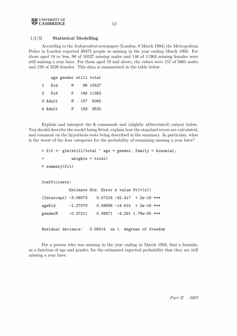
1/I/5I Statistical Modelling

According to the Independent newspaper (London, 8 March 1994) the MetropolitanPolice in London reported 30475 people as missing in the year ending March 1993. Forthose aged 18 or less, 96 of 10527 missing males and 146 of 11363 missing females werestill missing a year later. For those aged 19 and above, the values were 157 of 5065 malesand 159 of 3520 females. This data is summarised in the table below.

age gender still total

1 Kid M 96 10527

2 Kid F 146 11363

3 Adult M 157 5065

4 Adult F 159 3520

Explain and interpret the R commands and (slightly abbreviated) output below.You should describe the model being fitted, explain how the standard errors are calculated,and comment on the hypothesis tests being described in the summary. In particular, whatis the worst of the four categories for the probability of remaining missing a year later?

> fit <- glm(still/total ~ age + gender, family = binomial,

+ weights = total)

> summary(fit)

Coefficients:


(Intercept) -3.06073 0.07216 -42.417 < 2e-16 ***

ageKid -1.27079 0.08698 -14.610 < 2e-16 ***

genderM -0.37211 0.08671 -4.291 1.78e-05 ***


For a person who was missing in the year ending in March 1993, find a formula,as a function of age and gender, for the estimated expected probability that they are stillmissing a year later.

Part II 2007

13

1/II/13I Statistical Modelling

This problem deals with data collected as the number of each of two different strainsof Ceriodaphnia organisms are counted in a controlled environment in which reproductionis occurring among the organisms. The experimenter places into the containers a varyingconcentration of a particular component of jet fuel that impairs reproduction. Hence itis anticipated that as the concentration of jet fuel grows, the mean number of organismsshould decrease.

The table below gives a subset of the data. The full dataset has n = 70 rows. Thefirst column provides the number of organisms, the second the concentration of jet fuel(in grams per litre) and the third specifies the strain of the organism.

number fuel strain

82 0 1

58 0 0

45 0.5 1

27 0.5 0

29 0.75 1

15 1.25 1

6 1.25 1

8 1.5 0

4 1.75 0

. . .

. . .

Explain and interpret the R commands and (slightly abbreviated) output below. Inparticular, you should describe the model being fitted, explain how the standard errorsare calculated, and comment on the hypothesis tests being described in the summary.

> fit1 <- glm(number ~ fuel + strain + fuel:strain,family = poisson)

> summary(fit1)

Coefficients:


(Intercept) 4.14443 0.05101 81.252 < 2e-16 ***

fuel -1.47253 0.07007 -21.015 < 2e-16 ***

strain 0.33667 0.06704 5.022 5.11e-07 ***

fuel:strain -0.12534 0.09385 -1.336 0.182

The following R code fits two very similar models. Briefly explain the differencebetween these models and the one above. Motivate the fitting of these models in light of

Part II 2007

14

the summary from the fit of the one above.

> fit2 <- glm(number ~ fuel + strain, family = poisson)

> fit3 <- glm(number ~ fuel, family = poisson)

Denote by H1, H2, H3 the three hypotheses being fitted in sequence above.

Explain the hypothesis tests, including an approximate test of the fit of H1, thatcan be performed using the output from the following R code. Use these numbers tocomment on the most appropriate model for the data.

> c(fit1$dev, fit2$dev, fit3$dev)

[1] 84.59557 86.37646 118.99503

> qchisq(0.95, df = 1)

[1] 3.841459


Consider the linear regression setting where the responses Yi, i = 1, . . . , n areassumed independent with means µi = xT

i β. Here xi is a vector of known explanatoryvariables and β is a vector of unknown regression coefficients.

Show that if the response distribution is Laplace, i.e.,

Yi ∼ f(yi;µi, σ) = (2σ)−1 exp−|yi − µi|

σ

, i = 1, . . . , n; yi, µi ∈ R; σ ∈ (0,∞);

then the maximum likelihood estimate β of β is obtained by minimising

S1(β) =n∑

i=1

|Yi − xTi β|.

Obtain the maximum likelihood estimate for σ in terms of S1(β).

Briefly comment on why the Laplace distribution cannot be written in exponentialdispersion family form.

Part II 2007

15


Consider two possible experiments giving rise to observed data yij wherei = 1, . . . , I, j = 1, . . . , J .

1. The data are realizations of independent Poisson random variables, i.e.,

Yij ∼ f1(yij ;µij) =µ

yij

ij

yij !exp−µij

where µij = µij(β), with β an unknown (possibly vector) parameter. Write β forthe maximum likelihood estimator (m.l.e.) of β and yij = µij(β) for the (i, j)thfitted value under this model.

2. The data are components of a realization of a multinomial random ‘vector’

Y ∼ f2((yij);n, (pij)) = n!I∏

i=1

J∏j=1

pyij

ij

yij !

where the yij are non-negative integers with

I∑i=1

J∑j=1

yij = n and pij(β) =µij(β)n

.

Write β∗ for the m.l.e. of β and y∗ij = npij(β∗) for the (i, j)th fitted value underthis model.

Show that, ifI∑

i=1

J∑j=1

yij = n ,

then β = β∗ and yij = y∗ij for all i, j. Explain the relevance of this result in the contextof fitting multinomial models within a generalized linear model framework.

Part II 2007

16


Consider the normal linear model Y = Xβ + ε in vector notation, where

Y =

Y1...Yn

, X =

xT1...xT

n

, β =

β1...βp

, ε =

ε1...εn

, εi ∼ i.i.d. N(0, σ2),

where xTi = (xi1, . . . , xip) is known and X is of full rank (p < n). Give expressions for

maximum likelihood estimators β and σ2 of β and σ2 respectively, and state their jointdistribution.

Suppose that there is a new pair (x∗, y∗), independent of (x1, y1), . . . , (xn, yn),satisfying the relationship

y∗ = x∗Tβ + ε∗, where ε∗ ∼ N(0, σ2).

We suppose that x∗ is known, and estimate y∗ by y = x∗Tβ. State the distribution of

y − y∗

στ, where σ2 =

n

n− pσ2 and τ2 = x∗T(XTX)−1x∗ + 1.

Find the form of a (1− α)–level prediction interval for y∗.


Let Y have a Gamma distribution with density

f(y;α, λ) =λαyα−1

Γ(α)e−λy .

Show that the Gamma distribution is of exponential dispersion family form. Deducedirectly the corresponding expressions for E[Y ] and Var[Y ] in terms of α and λ. What isthe canonical link function?

Let p < n. Consider a generalised linear model (g.l.m.) for responses yi, i = 1, . . . , nwith random component defined by the Gamma distribution with canonical link g(µ), sothat g(µi) = ηi = xT

i β, where β = (β1, . . . , βp)T is the vector of unknown regressioncoefficients and xi = (xi1, . . . , xip)T is the vector of known values of the explanatoryvariables for the ith observation, i = 1, . . . , n.

Obtain expressions for the score function and Fisher information matrix and explainhow these can be used in order to approximate β, the maximum likelihood estimator(m.l.e.) of β.

[Use the canonical link function and assume that the dispersion parameter is known.]

Finally, obtain an expression for the deviance for a comparison of the full (sat-urated) model to the g.l.m. with canonical link using the m.l.e. β (or estimated meanµ = Xβ).

Part II 2007

10


Assume that observations Y = (Y1, . . . , Yn)T satisfy the linear model

Y = Xβ + ε,

where X is an n×p matrix of known constants of full rank p < n, where β = (β1, . . . , βp)T

is unknown and ε ∼ Nn(0, σ2I). Write down a (1− α)-level confidence set for β.

Define Cook’s distance for the observation (xi, Yi), where xTi is the ith row of X.

Give its interpretation in terms of confidence sets for β.

In the above model with n = 50 and p = 2, you observe that one observation hasCook’s distance 1.3. Would you be concerned about the influence of this observation?

[You may find some of the following facts useful:(i) If Z ∼ χ2

2, then P(Z 6 0.21) = 0.1, P(Z 6 1.39) = 0.5 and P(Z 6 4.61) = 0.9.(ii) If Z ∼ F2,48, then P(Z 6 0.11) = 0.1, P(Z 6 0.70) = 0.5 and P(Z 6 2.42) = 0.9.(iii) If Z ∼ F48,2, then P(Z 6 0.41) = 0.1, P(Z 6 1.42) = 0.5 and P(Z 6 9.47) = 0.9. ]

Part II 2006

11


The table below gives a year-by-year summary of the career batting record of thebaseball player Babe Ruth. The first column gives his age at the start of each season andthe second gives the number of ‘At Bats’ (AB) he had during the season. For each At Bat,it is recorded whether or not he scored a ‘Hit’. The third column gives the total numberof Hits he scored in the season, and the final column gives his ‘Average’ for the season,defined as the number of Hits divided by the number of At Bats.

Age AB Hits Average

19 10 2 0.200

20 92 29 0.315

21 136 37 0.272

22 123 40 0.325

23 317 95 0.300

24 432 139 0.322

25 457 172 0.376

26 540 204 0.378

27 406 128 0.315

28 522 205 0.393

29 529 200 0.378

30 359 134 0.373

31 495 184 0.372

32 540 192 0.356

33 536 173 0.323

34 499 172 0.345

35 518 186 0.359

36 534 199 0.373

37 457 156 0.341

38 459 138 0.301

39 365 105 0.288

40 72 13 0.181

Part II 2006

12

Explain and interpret the R commands below. In particular, you should explainthe model that is being fitted, the approximation leading to the given standard errors andthe test that is being performed in the last line of output.

> Mod <- glm(Hits/AB~Age+I(Age^2),family=binomial,weights=AB)

> summary(Mod)

Coefficients:


(Intercept) -4.5406713 0.8487687 -5.350 8.81e-08 ***

Age 0.2684739 0.0565992 4.743 2.10e-06 ***

I(Age^2) -0.0044827 0.0009253 -4.845 1.27e-06 ***


Assuming that any required packages are loaded, draw a careful sketch of the graphthat you would expect to see on entering the following lines of code:

> Coef <- coef(Mod)

> Fitted <- inv.logit(Coef[[1]]+Coef[[2]]*Age+Coef[[3]]*Age^2)

> plot(Age,Average)

> lines(Age,Fitted)


Let Y1, . . . , Yn be independent Poisson random variables with means µ1, . . . , µn, fori = 1, . . . , n, where log(µi) = βxi, for some known constants xi and an unknown parameterβ. Find the log-likelihood for β.

By first computing the first and second derivatives of the log-likelihood for β,explain the algorithm you would use to find the maximum likelihood estimator, β.

Part II 2006

13


Consider a generalized linear model for independent observations Y1, . . . , Yn, withE(Yi) = µi for i = 1, . . . , n. What is a linear predictor? What is meant by the linkfunction? If Yi has model function (or density) of the form

f(yi;µi, σ2) = exp

[1σ2

θ(µi)yi −K(θ(µi))

]a(σ2, yi),

for yi ∈ Y ⊆ R, µi ∈ M ⊆ R, σ2 ∈ Φ ⊆ (0,∞), where a(σ2, yi) is a known positivefunction, define the canonical link function.

Now suppose that Y1, . . . , Yn are independent with Yi ∼ Bin(1, µi) for i = 1, . . . , n.Derive the canonical link function.

Part II 2006

14


The table below summarises the yearly numbers of named storms in the Atlanticbasin over the period 1944–2004, and also gives an index of average July ocean temperaturein the northern hemisphere over the same period. To save space, only the data for thefirst four and last four years are shown.

Year Storms Temp

1944 11 0.165

1945 11 0.080

1946 6 0.000

1947 9 -0.024

......

...

2001 15 0.592

2002 12 0.627

2003 16 0.608

2004 15 0.546

Explain and interpret the R commands and (slightly abbreviated) output below.

> Mod <- glm(Storms~Temp,family=poisson)

> summary(Mod)

Coefficients:


(Intercept) 2.26061 0.04841 46.697 < 2e-16 ***

Temp 0.48870 0.16973 2.879 0.00399 **


In 2005, the ocean temperature index was 0.743. Explain how you would predictthe number of named storms for that year.

Part II 2006

15


Consider a linear model for Y = (Y1, . . . , Yn)T given by

Y = Xβ + ε,

where X is a known n × p matrix of full rank p < n, where β is an unknown vector andε ∼ Nn(0, σ2I). Derive an expression for the maximum likelihood estimator β of β, andwrite down its distribution.

Find also the maximum likelihood estimator σ2 of σ2, and derive its distribution.

[You may use Cochran’s theorem, provided that it is stated carefully. You may also assumethat the matrix P = X(XTX)−1XT has rank p, and that I − P has rank n− p.]

Part II 2006

10


Suppose that Y1, . . . , Yn are independent random variables, and that Yi has prob-ability density function

f(yi|θi, φ) = exp[ (yiθi − b(θi))

φ+ c(yi, φ)

].

Assume that E(Yi) = µi and that there is a known link function g(.) such that

g(µi) = βTxi ,

where x1, . . . , xn are known p-dimensional vectors and β is an unknown p-dimensionalparameter. Show that E(Yi) = b′(θi) and that, if `(β, φ) is the log-likelihood functionfrom the observations (y1, . . . , yn), then

∂`(β, φ)∂β

=n∑1

(yi − µi)xi

g′(µi)Vi,

where Vi is to be defined.


The Independent, June 1999, under the headline ‘Tourists get hidden costs warn-ings’ gave the following table of prices in pounds, called ‘How the resorts compared’.

Algarve 8.00 0.50 3.50 3.00 4.00 100.00

CostaDelSol 6.95 1.30 4.10 12.30 4.10 130.85

Majorca 10.25 1.45 5.35 6.15 3.30 122.20

Tenerife 12.30 1.25 4.90 3.70 2.90 130.85

Florida 15.60 1.90 5.05 5.00 2.50 114.00

Tunisia 10.90 1.40 5.45 1.90 2.75 218.10

Cyprus 11.60 1.20 5.95 3.00 3.60 149.45

Turkey 6.50 1.05 6.50 4.90 2.85 263.00

Corfu 5.20 1.05 3.75 4.20 2.50 137.60

Sorrento 7.70 1.40 6.30 8.75 4.75 215.40

Malta 11.20 0.70 4.55 8.00 4.80 87.85

Rhodes 6.30 1.05 5.20 3.15 2.70 261.30

Sicily 13.25 1.75 4.20 7.00 3.85 174.40

Madeira 10.25 0.70 5.10 6.85 6.85 153.70

Part II 2005

11

Here the column headings are, respectively: Three-course meal, Bottle of Beer,Suntan Lotion, Taxi (5km), Film (24 exp), Car Hire (per week). Interpret the Rcommands, and explain how to interpret the corresponding (slightly abbreviated) R outputgiven below. Your solution should include a careful statement of the underlying statisticalmodel, but you may quote without proof any distributional results required.

> price = scan("dresorts") ; price

> Goods = gl(6,1,length=84); Resort=gl(14,6,length=84)

> first.lm = lm(log(price) ~ Goods + Resort)

> summary(first.lm)

Coefficients:


(Intercept) 1.8778 0.1629 11.527 < 2e-16

Goods2 -2.1084 0.1295 -16.286 < 2e-16

Goods3 -0.6343 0.1295 -4.900 6.69e-06

Goods4 -0.6284 0.1295 -4.854 7.92e-06

Goods5 -0.9679 0.1295 -7.476 2.49e-10

Goods6 2.8016 0.1295 21.640 < 2e-16

Resort2 0.4463 0.1978 2.257 0.02740

Resort3 0.4105 0.1978 2.076 0.04189

Resort4 0.3067 0.1978 1.551 0.12584

Resort5 0.4235 0.1978 2.142 0.03597

Resort6 0.2883 0.1978 1.458 0.14963

Resort7 0.3457 0.1978 1.748 0.08519

Resort8 0.3787 0.1978 1.915 0.05993

Resort9 0.0943 0.1978 0.477 0.63508

Resort10 0.5981 0.1978 3.025 0.00356

Resort11 0.3281 0.1978 1.659 0.10187

Resort12 0.2525 0.1978 1.277 0.20616

Resort13 0.5508 0.1978 2.785 0.00700

Resort14 0.4590 0.1978 2.321 0.02343


Multiple R-Squared: 0.962

Part II 2005

12


You see below three R commands, and the corresponding output (which is slightlyabbreviated). Explain the effects of the commands. How is the deviance defined, and whydo we have d.f.=7 in this case? Interpret the numerical values found in the output.

> n = scan()

3 5 16 12 11 34 37 51 56

> i = scan ()

1 2 3 4 5 6 7 8 9

> summary(glm(n~i,poisson))

deviance = 13.218

d.f. = 7

Coefficients:

Value Std.Error

(intercept) 1.363 0.2210

i 0.3106 0.0382


Consider the model Y = Xβ + ε, where Y is an n-dimensional observation vector,X is an n× p matrix of rank p, ε is an n-dimensional vector with components ε1, . . . , εn,and ε1, . . . , εn are independently and normally distributed, each with mean 0 and varianceσ2.

(a) Let β be the least-squares estimator of β. Show that

(XTX)β = XTY

and find the distribution of β.

(b) Define Y = Xβ. Show that Y has distribution N(Xβ, σ2H), where H is amatrix that you should define.

[You may quote without proof any results you require about the multivariate normaldistribution.]

Part II 2005

13


You see below five R commands, and the corresponding output (which is slightlyabbreviated). Without giving any mathematical proofs, explain the purpose of thesecommands, and interpret the output.

> Yes = c(12, 27,11,24)

> Total = c(117,170,52,118)

> Sclass = c("a","a","b","b")

> Sclass = factor(Sclass)

> summary(glm(Yes/Total~ Sclass, binomial, weights=Total))

Coefficients:

Estimate Std. Error z value

(Intercept) -1.8499 0.1723 -10.739

Sclassb 0.4999 0.2562 1.951



Part II 2005

14


(i) Suppose that Y1, . . . , Yn are independent random variables, and that Yi hasprobability density function

f(yi|β, ν) =(νyi

µi

)ν

e−yiν/µi1

Γ(ν)1yi

for yi > 0

where1/µi = βTxi , for 1 6 i 6 n,

and x1, . . . , xn are given p-dimensional vectors, and ν is known.

Show that E(Yi) = µi and that var (Yi) = µ2i /ν.

(ii) Find the equation for β, the maximum likelihood estimator of β, and suggestan iterative scheme for its solution.

(iii) If p = 2, and xi =(

1zi

), find the large-sample distribution of β2. Write your

answer in terms of a, b, c and ν, where a, b, c are defined by

a =∑

µ2i , b =

∑ziµ

2i , c =

∑z2i µ

2i .

Part II 2005

9

A1/13 Computational Statistics and Statistical Modelling

(i) Assume that the n-dimensional vector Y may be written as Y = Xβ+ ε, where Xis a given n× p matrix of rank p, β is an unknown vector, and

ε ∼ Nn(0, σ2I).

Let Q(β) = (Y − Xβ)T (Y − Xβ). Find β, the least-squares estimator of β, and statewithout proof the joint distribution of β and Q(β).

(ii) Now suppose that we have observations (Yij , 1 6 i 6 I, 1 6 j 6 J) and considerthe model

Ω : Yij = µ+ αi + βj + εij ,

where (αi), (βj) are fixed parameters with Σαi = 0, Σβj = 0, and (εij) may be assumedindependent normal variables, with εij ∼ N(0, σ2), where σ2 is unknown.

(a) Find (αi), (βj), the least-squares estimators of (αi), (βj).

(b) Find the least-squares estimators of (αi) under the hypothesis H0 : βj = 0 forall j.

(c) Quoting any general theorems required, explain carefully how to test H0,assuming Ω is true.

(d) What would be the effect of fitting the model Ω1 : Yij = µ+αi + βj + γij + εij ,where now (αi), (βj), (γij) are all fixed unknown parameters, and (εij) has the distributiongiven above?


(i) Suppose we have independent observations Y1, . . . , Yn, and we assume that fori = 1, . . . , n, Yi is Poisson with mean µi, and log(µi) = βTxi, where x1, . . . , xn are givencovariate vectors each of dimension p, where β is an unknown vector of dimension p,and p < n. Assuming that x1, . . . , xn span Rp, find the equation for β, the maximumlikelihood estimator of β, and write down the large-sample distribution of β.

(ii) A long-term agricultural experiment had 90 grassland plots, each 25m × 25m,differing in biomass, soil pH, and species richness (the count of species in the whole plot).While it was well-known that species richness declines with increasing biomass, it was notknown how this relationship depends on soil pH, which for the given study has possiblevalues “low”, “medium” or “high”, each taken 30 times. Explain the commands input, andinterpret the resulting output in the (slightly edited) R output below, in which “species”represents the species count.

(The first and last 2 lines of the data are reproduced here as an aid. You mayassume that the factor pH has been correctly set up.)

Part II 2004

10

> species

pH Biomass Species

1 high 0.46929722 30

2 high 1.73087043 39

.......................

.......................

89 low 4.36454121 7

90 low 4.87050789 3

> summary(glm(Species ~Biomass, family = poisson))

Call:

glm(formula = Species ~ Biomass, family = poisson)

Coefficients:


(Intercept) 3.184094 0.039159 81.31 < 2e-16

Biomass -0.064441 0.009838 -6.55 5.74e-11

(Dispersion parameter for poisson family taken to be 1)




> summary(glm(Species ~pH*Biomass, family = poisson))

Call:

glm(formula = Species ~ pH * Biomass, family = poisson)

Coefficients:


(Intercept) 3.76812 0.06153 61.240 < 2e-16

pHlow -0.81557 0.10284 -7.931 2.18e-15

Question continues on next page.

Part II 2004

11

pHmid -0.33146 0.09217 -3.596 0.000323

Biomass -0.10713 0.01249 -8.577 < 2e-16

pHlow:Biomass -0.15503 0.04003 -3.873 0.000108

pHmid:Biomass -0.03189 0.02308 -1.382 0.166954





Part II 2004

12


Suppose that Y1, . . . , Yn are independent observations, with Yi having probabilitydensity function of the following form

f(yi|θi, φ) = exp[yiθi − b(θi)

φ+ c(yi, φ)

]where E(Yi) = µi and g(µi) = βTxi. You should assume that g( ) is a known function,and β, φ are unknown parameters, with φ > 0, and also x1, . . . , xn are given linearlyindependent covariate vectors. Show that

∂`

∂β=

∑ (yi − βi)g′(µi)Vi

xi,

where ` is the log-likelihood and Vi = var (Yi) = φb′′(θi).

Discuss carefully the (slightly edited) R output given below, and briefly suggestanother possible method of analysis using the function glm ( ).

> s <- scan()

1: 33 63 157 38 108 159

7:

Read 6 items

> r <- scan()

1: 3271 7256 5065 2486 8877 3520

7:

Read 6 items

> gender <- scan(,"")

1: b b b g g g

7:

Read 6 items

> age <- scan(,"")

1: 13&under 14-18 19&over

4: 13&under 14-18 19&over

7:

Read 6 items

> gender <- factor(gender) ; age <- factor(age)

> summary(glm(s/r ~ gender + age,binomial, weights=r))

Coefficients:

Question continues on next page.

Part II 2004

13

Estimate Std.Error z-value Pr(>|z|)

(Intercept) -4.56479 0.12783 -35.710 < 2e-16

genderg 0.38028 0.08689 4.377 1.21e-05

age14-18 -0.19797 0.14241 -1.390 0.164

age19&over 1.12790 0.13252 8.511 < 2e-16





Part II 2004

9


(i) Suppose Yi, 1 6 i 6 n, are independent binomial observations, with Yi ∼ Bi(ti, πi),1 6 i 6 n, where t1, . . . , tn are known, and we wish to fit the model

ω : logπi

1− πi= µ+ βTxi for each i,

where x1, . . . , xn are given covariates, each of dimension p. Let µ, β be the maximumlikelihood estimators of µ, β. Derive equations for µ, β and state without proof the formof the approximate distribution of β.

(ii) In 1975, data were collected on the 3-year survival status of patients suffering froma type of cancer, yielding the following table

survive?age in years malignant yes no

under 50 no 77 10under 50 yes 51 13

50-69 no 51 1150-69 yes 38 2070+ no 7 370+ yes 6 3

Here the second column represents whether the initial tumour was not malignant or wasmalignant.

Let Yij be the number surviving, for age group i and malignancy status j, fori = 1, 2, 3 and j = 1, 2, and let tij be the corresponding total number. Thus Y11 = 77,t11 = 87. Assume Yij ∼ Bi(tij , πij), 1 6 i 6 3, 1 6 j 6 2. The results from fitting themodel

log(πij/(1− πij)) = µ+ αi + βj

with α1 = 0, β1 = 0 give β2 = −0.7328 (se = 0.2985), and deviance = 0.4941. What doyou conclude?

Why do we take α1 = 0, β1 = 0 in the model?

What “residuals” should you compute, and to which distribution would you referthem?

Part II 2003

10


(i) Suppose Y1, . . . , Yn are independent Poisson variables, and

E(Yi) = µi , logµi = α+ βti , for i = 1, . . . , n ,

where α, β are two unknown parameters, and t1, . . . , tn are given covariates, each ofdimension 1. Find equations for α, β, the maximum likelihood estimators of α, β, andshow how an estimate of var(β) may be derived, quoting any standard theorems you mayneed.

(ii) By 31 December 2001, the number of new vCJD patients, classified by reportedcalendar year of onset, were

8, 10, 11, 14, 17, 29, 23

for the years1994, . . . , 2000 respectively.

Discuss carefully the (slightly edited) R output for these data given below, quotingany standard theorems you may need.

> year

year

[1] 1994 1995 1996 1997 1998 1999 2000

> tot

[1] 8 10 11 14 17 29 23

>first.glm _ glm(tot ~ year, family = poisson)

> summary(first.glm)

Call:

glm(formula = tot ~ year, family = poisson)

Coefficients


(Intercept) -407.81285 99.35366 -4.105 4.05e-05

year 0.20556 0.04973 4.133 3.57e-05





Part II 2003

11


The nave height x, and the nave length y for 16 Gothic-style cathedrals and 9Romanesque-style cathedrals, all in England, have been recorded, and the correspondingR output (slightly edited) is given below.

> first.lm _ lm(y ~ x + Style); summary(first.lm)

Call:

lm(formula = y ~ x + Style)

Residuals:

Min 1Q Median 3Q Max

-172.67 -30.44 20.38 55.02 96.50

Coefficients:


(Intercept) 44.298 81.648 0.543 0.5929

x 4.712 1.058 4.452 0.0002

Style2 80.393 32.306 2.488 0.0209



You may assume that x, y are in suitable units, and that “style” has been set upas a factor with levels 1,2 corresponding to Gothic, Romanesque respectively.

(a) Explain carefully, with suitable graph(s) if necessary, the results of this analysis.

(b) Using the general model Y = Xβ + ε (in the conventional notation) explaincarefully the theory needed for (a).

[Standard theorems need not be proved.]

Part II 2003

8


(i) Suppose Y1, . . . , Yn are independent Poisson variables, and

E(Yi) = µi , logµi = α+ βTxi , 1 6 i 6 n

where α, β are unknown parameters, and x1, . . . , xn are given covariates, each of dimensionp. Obtain the maximum-likelihood equations for α, β, and explain briefly how you wouldcheck the validity of this model.

(ii) The data below show y1, . . . , y33, which are the monthly accident counts on amajor US highway for each of the 12 months of 1970, then for each of the 12 months of1971, and finally for the first 9 months of 1972. The data-set is followed by the (slightlyedited) R output. You may assume that the factors ‘Year’ and ‘month’ have been set upin the appropriate fashion. Give a careful interpretation of this R output, and explain (a)how you would derive the corresponding standardised residuals, and (b) how you wouldpredict the number of accidents in October 1972.

52 37 49 29 31 32 28 34 32 39 50 6335 22 27 27 34 23 42 30 36 56 48 4033 26 31 25 23 20 25 20 36

> first.glm glm(y∼ Year + month, poisson) ; summary(first.glm)

Call:

glm(formula = y ∼ Year + month, family = poisson)

Coefficients:Estimate Std. Error z value Pr(> |z|)

(Intercept) 3.81969 0.09896 38.600 < 2e− 16 ***Year1971 -0.12516 0.06694 -1.870 0.061521 .Year1972 -0.28794 0.08267 -3.483 0.000496 ***month2 -0.34484 0.14176 -2.433 0.014994 *month3 -0.11466 0.13296 -0.862 0.388459month4 -0.39304 0.14380 -2.733 0.006271 **month5 -0.31015 0.14034 -2.210 0.027108 *month6 -0.47000 0.14719 -3.193 0.001408 **month7 -0.23361 0.13732 -1.701 0.088889 .month8 -0.35667 0.14226 -2.507 0.012168 *month9 -0.14310 0.13397 -1.068 0.285444month10 0.10167 0.13903 0.731 0.464628month11 0.13276 0.13788 0.963 0.335639month12 0.18252 0.13607 1.341 0.179812

Signif. codes: 0 ‘***’ 0.001 ‘**’ 0.01 ‘*’ 0.05 ‘.’


Null deviance: 101.143 on 32 degrees of freedomResidual deviance: 27.273 on 19 degrees of freedom


Part II 2002

9


(i) Suppose that the random variable Y has density function of the form

f(y|θ, φ) = exp[yθ − b(θ)

φ+ c(y, φ)

]where φ > 0. Show that Y has expectation b′(θ) and variance φb′′(θ).

(ii) Suppose now that Y1, . . . , Yn are independent negative exponential variables, withYi having density function f(yi|µi) = 1

µie−yi/µi for yi > 0. Suppose further that

g(µi) = βTxi for 1 6 i 6 n, where g(·) is a known ‘link’ function, and x1, . . . , xn aregiven covariate vectors, each of dimension p. Discuss carefully the problem of finding β,the maximum-likelihood estimator of β, firstly for the case g(µi) = 1/µi, and secondly forthe case g(µ) = logµi; in both cases you should state the large-sample distribution of β.

[Any standard theorems used need not be proved.]


Assume that the n-dimensional observation vector Y may be written as Y = Xβ+ε,where X is a given n×p matrix of rank p, β is an unknown vector, with βT = (β1, . . . , βp),and

ε ∼ Nn(0, σ2I) (∗)

where σ2 is unknown. Find β, the least-squares estimator of β, and describe (withoutproof) how you would test

H0 : βν = 0

for a given ν.

Indicate briefly two plots that you could use as a check of the assumption (∗).Continued opposite

Part II 2002

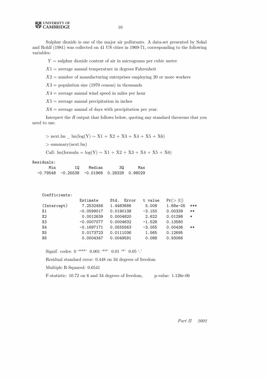
10

Sulphur dioxide is one of the major air pollutants. A data-set presented by Sokaland Rohlf (1981) was collected on 41 US cities in 1969-71, corresponding to the followingvariables:

Y = sulphur dioxide content of air in micrograms per cubic metre

X1 = average annual temperature in degrees Fahrenheit

X2 = number of manufacturing enterprises employing 20 or more workers

X3 = population size (1970 census) in thousands

X4 = average annual wind speed in miles per hour

X5 = average annual precipitation in inches

X6 = average annual of days with precipitation per year.

Interpret the R output that follows below, quoting any standard theorems that youneed to use.

> next.lm lm(log(Y) ∼ X1 + X2 + X3 + X4 + X5 + X6)

> summary(next.lm)

Call: lm(formula = log(Y) ∼ X1 + X2 + X3 + X4 + X5 + X6)

Residuals:Min 1Q Median 3Q Max

-0.79548 -0.25538 -0.01968 0.28328 0.98029

Coefficients:Estimate Std. Error t value Pr(> |t|)

(Intercept) 7.2532456 1.4483686 5.008 1.68e-05 ***X1 -0.0599017 0.0190138 -3.150 0.00339 **X2 0.0012639 0.0004820 2.622 0.01298 *X3 -0.0007077 0.0004632 -1.528 0.13580X4 -0.1697171 0.0555563 -3.055 0.00436 **X5 0.0173723 0.0111036 1.565 0.12695X6 0.0004347 0.0049591 0.088 0.93066

Signif. codes: 0 ‘***’ 0.001 ‘**’ 0.01 ‘*’ 0.05 ‘.’



F-statistic: 10.72 on 6 and 34 degrees of freedom, p-value: 1.126e-06

Part II 2002

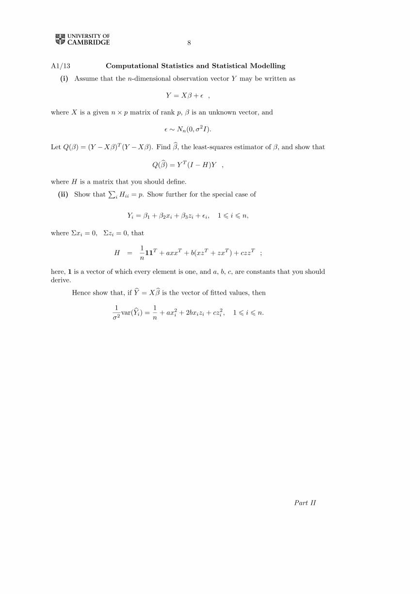
8


(i) Assume that the n-dimensional observation vector Y may be written as

Y = Xβ + ε ,

where X is a given n× p matrix of rank p, β is an unknown vector, and

ε ∼ Nn(0, σ2I).

Let Q(β) = (Y −Xβ)T (Y −Xβ). Find β, the least-squares estimator of β, and show that

Q(β) = Y T (I −H)Y ,

where H is a matrix that you should define.

(ii) Show that∑iHii = p. Show further for the special case of

Yi = β1 + β2xi + β3zi + εi, 1 6 i 6 n,

where Σxi = 0, Σzi = 0, that

H =1n11T + axxT + b(xzT + zxT ) + czzT ;

here, 1 is a vector of which every element is one, and a, b, c, are constants that you shouldderive.

Hence show that, if Y = Xβ is the vector of fitted values, then

1σ2

var(Yi) =1n

+ ax2i + 2bxizi + cz2

i , 1 6 i 6 n.

Part II

9


(i) Suppose that Y1, . . . , Yn are independent random variables, and that Yi hasprobability density function

f(yi|θi, φ) = exp[(yiθi − b(θi))/φ+ c(yi, φ)].

Assume that E(Yi) = µi, and that g(µi) = βTxi, where g(·) is a known ‘link’ function,x1, . . . , xn are known covariates, and β is an unknown vector. Show that

E(Yi) = b′(θi), var(Yi) = φb′′(θi) = Vi, say,

and hence

∂l

∂β=

n∑i=1

(yi − µi)xig′(µi)Vi

, where l = l(β, φ) is the log-likelihood.

(ii) The table below shows the number of train miles (in millions) and the number ofcollisions involving British Rail passenger trains between 1970 and 1984. Give a detailedinterpretation of the R output that is shown under this table:

year collisions miles1 1970 3 2812 1971 6 2763 1972 4 2684 1973 7 2695 1974 6 2816 1975 2 2717 1976 2 2658 1977 4 2649 1978 1 26710 1979 7 26511 1980 3 26712 1981 5 26013 1982 6 23114 1983 1 249

Call:

glm(formula = collisions ∼ year + log(miles), family = poisson)

Coefficients:Estimate Std. Error z value Pr(>|z|)

(Intercept) 127.14453 121.37796 1.048 0.295year -0.05398 0.05175 -1.043 0.297log(miles) -3.41654 4.18616 -0.816 0.414





Part II

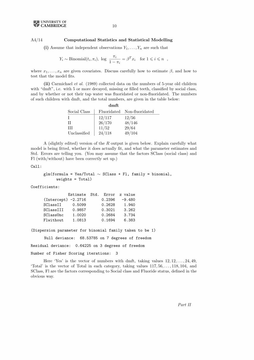
10


(i) Assume that independent observations Y1, . . . , Yn are such that

Yi ∼ Binomial(ti, πi), logπi

1− πi= βTxi for 1 6 i 6 n ,

where x1, . . . , xn are given covariates. Discuss carefully how to estimate β, and how totest that the model fits.

(ii) Carmichael et al. (1989) collected data on the numbers of 5-year old childrenwith “dmft”, i.e. with 5 or more decayed, missing or filled teeth, classified by social class,and by whether or not their tap water was fluoridated or non-fluoridated. The numbersof such children with dmft, and the total numbers, are given in the table below:

dmftSocial Class Fluoridated Non-fluoridatedI 12/117 12/56II 26/170 48/146III 11/52 29/64Unclassified 24/118 49/104

A (slightly edited) version of the R output is given below. Explain carefully whatmodel is being fitted, whether it does actually fit, and what the parameter estimates andStd. Errors are telling you. (You may assume that the factors SClass (social class) andFl (with/without) have been correctly set up.)

Call:

glm(formula = Yes/Total ∼ SClass + Fl, family = binomial,weights = Total)

Coefficients:

Estimate Std. Error z value(Intercept) -2.2716 0.2396 -9.480SClassII 0.5099 0.2628 1.940SClassIII 0.9857 0.3021 3.262SClassUnc 1.0020 0.2684 3.734Flwithout 1.0813 0.1694 6.383





Here ‘Yes’ is the vector of numbers with dmft, taking values 12, 12, . . . , 24, 49,‘Total’ is the vector of Total in each category, taking values 117, 56, . . . , 118, 104, andSClass, Fl are the factors corresponding to Social class and Fluoride status, defined in theobvious way.

Part II

88rds37/teaching/statistical...88 Paper 4, Section I 5K Statistical Modelling Consider the normal...

Documents

Transcript of 88rds37/teaching/statistical...88 Paper 4, Section I 5K Statistical Modelling Consider the normal...