· 8 November, 2005 Determination of Neutrino Mixing-Angle µ13 Using The Daya Bay Nuclear Power...
189
8 November, 2005 Determination of Neutrino Mixing-Angle θ 13 Using The Daya Bay Nuclear Power Facilities Version 3.2 Beijing Normal University, China Chinese University of Hong Kong, China Institute of Atomic Energy, China Institute of High Energy Physics, China Institute for Scintillation Materials, Ukraine Institute of Theoretical Physics, China Iowa State University, U.S.A. Joint Institute for Nuclear Research at Dubna, Russia Kurchatov Institute, Russia Lawrence Berkeley National Laboratory, U.S.A. Nankai University, China Shenzhen University, China Sun Yat-Sen (Zhongshan) University, China Tsing Hua University, China University of California at Berkeley, U.S.A. University of California at Los Angeles, U.S.A. University of Hong Kong, China University of Houston, U.S.A. University of Illinois at Urbana-Champaign, U.S.A. University of Science and Technology of China, China
Transcript of · 8 November, 2005 Determination of Neutrino Mixing-Angle µ13 Using The Daya Bay Nuclear Power...
8 November, 2005
Determination of Neutrino Mixing-Angle θ13
UsingThe Daya Bay Nuclear Power Facilities
Version 3.2
Beijing Normal University, China
Chinese University of Hong Kong, China
Institute of Atomic Energy, China
Institute of High Energy Physics, China
Institute for Scintillation Materials, Ukraine
Institute of Theoretical Physics, China
Iowa State University, U.S.A.
Joint Institute for Nuclear Research at Dubna, Russia
Kurchatov Institute, Russia
Lawrence Berkeley National Laboratory, U.S.A.
Nankai University, China
Shenzhen University, China
Sun Yat-Sen (Zhongshan) University, China
Tsing Hua University, China
University of California at Berkeley, U.S.A.
University of California at Los Angeles, U.S.A.
University of Hong Kong, China
University of Houston, U.S.A.
University of Illinois at Urbana-Champaign, U.S.A.
University of Science and Technology of China, China

ii
Contents
1 Introduction 1
2 Physics Motivation 52.1 Current Status of neutrino oscillation . . . . . . . . . . . . . . . . . . . . . . 52.2 Theoretical expectations of θ13 . . . . . . . . . . . . . . . . . . . . . . . . . . 11
2.2.1 Expectations of θ13 from global three-neutrino analysis . . . . . . . . 112.2.2 Expectations of θ13 from specific neutrino mass models . . . . . . . . 13
2.3 Measurement of θ13 . . . . . . . . . . . . . . . . . . . . . . . . . . . . . . . . 152.3.1 Long-baseline experiments and the measurement θ13 . . . . . . . . . . 152.3.2 Advantages of measuring θ13 with reactors . . . . . . . . . . . . . . . 17
3 Reactor Antineutrino 293.1 Energy spectrum and flux of reactor antineutrinos . . . . . . . . . . . . . . . 303.2 Inverse beta decay . . . . . . . . . . . . . . . . . . . . . . . . . . . . . . . . 323.3 Prediction and observed antineutrino flux and spectrum . . . . . . . . . . . . 34
4 Experimental Site and Laboratory Designs 374.1 Overview . . . . . . . . . . . . . . . . . . . . . . . . . . . . . . . . . . . . . . 374.2 Site geology . . . . . . . . . . . . . . . . . . . . . . . . . . . . . . . . . . . . 394.3 Seismic activities . . . . . . . . . . . . . . . . . . . . . . . . . . . . . . . . . 394.4 Engineering geology . . . . . . . . . . . . . . . . . . . . . . . . . . . . . . . . 404.5 Hydrogeology . . . . . . . . . . . . . . . . . . . . . . . . . . . . . . . . . . . 404.6 Stability of mountain and cavern . . . . . . . . . . . . . . . . . . . . . . . . 424.7 Transportation . . . . . . . . . . . . . . . . . . . . . . . . . . . . . . . . . . 434.8 Design of laboratory facilities . . . . . . . . . . . . . . . . . . . . . . . . . . 43
4.8.1 Detector sites . . . . . . . . . . . . . . . . . . . . . . . . . . . . . . . 434.8.2 Tunnels . . . . . . . . . . . . . . . . . . . . . . . . . . . . . . . . . . 45
5 Detector 495.1 Overview . . . . . . . . . . . . . . . . . . . . . . . . . . . . . . . . . . . . . . 495.2 Monte Carlo simulation . . . . . . . . . . . . . . . . . . . . . . . . . . . . . . 525.3 Liquid scintillator . . . . . . . . . . . . . . . . . . . . . . . . . . . . . . . . . 535.4 Detector modules . . . . . . . . . . . . . . . . . . . . . . . . . . . . . . . . . 57
iii
iv CONTENTS
5.4.1 Module geometry and Energy resolution . . . . . . . . . . . . . . . . 57
5.4.2 Gamma catcher . . . . . . . . . . . . . . . . . . . . . . . . . . . . . . 58
5.4.3 Two-layer versus Three-layer detector . . . . . . . . . . . . . . . . . . 59
5.4.4 Oil buffer . . . . . . . . . . . . . . . . . . . . . . . . . . . . . . . . . 60
5.4.5 Containers . . . . . . . . . . . . . . . . . . . . . . . . . . . . . . . . . 62
5.5 Water buffer . . . . . . . . . . . . . . . . . . . . . . . . . . . . . . . . . . . . 62
5.5.1 Water-tank option . . . . . . . . . . . . . . . . . . . . . . . . . . . . 63
5.5.2 Water-pool option . . . . . . . . . . . . . . . . . . . . . . . . . . . . 65
5.6 Muon veto . . . . . . . . . . . . . . . . . . . . . . . . . . . . . . . . . . . . . 66
5.6.1 Water Cherenkov detector . . . . . . . . . . . . . . . . . . . . . . . . 66
5.6.2 Resistive Plate Chamber . . . . . . . . . . . . . . . . . . . . . . . . . 67
5.6.3 Scintillator-strip muon tracker . . . . . . . . . . . . . . . . . . . . . . 68
5.7 PMT Readout System . . . . . . . . . . . . . . . . . . . . . . . . . . . . . . 71
5.7.1 Specifications . . . . . . . . . . . . . . . . . . . . . . . . . . . . . . . 72
5.7.2 PMT readout module . . . . . . . . . . . . . . . . . . . . . . . . . . . 73
5.7.3 Muon-veto readout system . . . . . . . . . . . . . . . . . . . . . . . . 74
5.8 Trigger system . . . . . . . . . . . . . . . . . . . . . . . . . . . . . . . . . . 75
5.9 Calibration . . . . . . . . . . . . . . . . . . . . . . . . . . . . . . . . . . . . 77
5.9.1 LED system . . . . . . . . . . . . . . . . . . . . . . . . . . . . . . . . 78
5.9.2 Laser system . . . . . . . . . . . . . . . . . . . . . . . . . . . . . . . 78
5.9.3 Radioactive sources . . . . . . . . . . . . . . . . . . . . . . . . . . . . 78
6 Detector Overburden and Backgrounds 83
6.1 Overburden and muon flux . . . . . . . . . . . . . . . . . . . . . . . . . . . . 84
6.2 Correlated background . . . . . . . . . . . . . . . . . . . . . . . . . . . . . . 87
6.2.1 Fast neutrons . . . . . . . . . . . . . . . . . . . . . . . . . . . . . . . 87
6.2.2 Cosmogenic 8He/9Li . . . . . . . . . . . . . . . . . . . . . . . . . . . 90
6.2.3 Other correlated backgrounds . . . . . . . . . . . . . . . . . . . . . . 93
6.3 Uncorrelated background . . . . . . . . . . . . . . . . . . . . . . . . . . . . . 94
6.4 Summary of backgrounds . . . . . . . . . . . . . . . . . . . . . . . . . . . . . 96
7 Systematic Issues 101
7.1 Overview . . . . . . . . . . . . . . . . . . . . . . . . . . . . . . . . . . . . . . 101
7.2 Systematic error estimates . . . . . . . . . . . . . . . . . . . . . . . . . . . . 103
7.2.1 Reactor power levels and locations . . . . . . . . . . . . . . . . . . . 103
7.2.2 Detector-related errors . . . . . . . . . . . . . . . . . . . . . . . . . . 105
7.2.3 Background . . . . . . . . . . . . . . . . . . . . . . . . . . . . . . . . 110
7.3 χ2 analysis . . . . . . . . . . . . . . . . . . . . . . . . . . . . . . . . . . . . 111
7.4 Side-by-side calibration and detector swapping . . . . . . . . . . . . . . . . 115
7.5 Baseline optimization . . . . . . . . . . . . . . . . . . . . . . . . . . . . . . . 117
7.6 Sensitivity . . . . . . . . . . . . . . . . . . . . . . . . . . . . . . . . . . . . . 119
CONTENTS v
8 Other Physics Reaches 1238.1 Sterile neutrinos . . . . . . . . . . . . . . . . . . . . . . . . . . . . . . . . . . 1238.2 Supernova Neutrinos and Supernova Watch . . . . . . . . . . . . . . . . . . . 126
8.2.1 SN neutrino spectra and flux . . . . . . . . . . . . . . . . . . . . . . 1278.2.2 Detect SN neutrinos in the Daya Bay experiment . . . . . . . . . . . 129
8.3 Exotic neutrino properties and nuclear power monitoring . . . . . . . . . . . 133
9 Research and Development 1379.1 Site survey . . . . . . . . . . . . . . . . . . . . . . . . . . . . . . . . . . . . 137
9.1.1 Topographic Survey . . . . . . . . . . . . . . . . . . . . . . . . . . . . 1379.1.2 Geological investigation . . . . . . . . . . . . . . . . . . . . . . . . . 1389.1.3 Geo-physical prospecting . . . . . . . . . . . . . . . . . . . . . . . . . 140
9.2 The Aberdeen Tunnel Laboratory . . . . . . . . . . . . . . . . . . . . . . . . 1439.2.1 Objective . . . . . . . . . . . . . . . . . . . . . . . . . . . . . . . . . 1439.2.2 Research plan and methodology . . . . . . . . . . . . . . . . . . . . . 1449.2.3 Anti-Radon painting . . . . . . . . . . . . . . . . . . . . . . . . . . . 149
9.3 Detector Prototype at IHEP . . . . . . . . . . . . . . . . . . . . . . . . . . . 1509.3.1 The Prototype . . . . . . . . . . . . . . . . . . . . . . . . . . . . . . 1509.3.2 PMT Test . . . . . . . . . . . . . . . . . . . . . . . . . . . . . . . . . 153
9.4 Liquid Scintillator . . . . . . . . . . . . . . . . . . . . . . . . . . . . . . . . . 1569.4.1 Introduction . . . . . . . . . . . . . . . . . . . . . . . . . . . . . . . . 1569.4.2 Gd-LS R&D at IHEP . . . . . . . . . . . . . . . . . . . . . . . . . . 1569.4.3 Future R&D at IHEP . . . . . . . . . . . . . . . . . . . . . . . . . . . 158
10 Strategy and Organization 16110.1 Run Plan . . . . . . . . . . . . . . . . . . . . . . . . . . . . . . . . . . . . . 161
10.1.1 Near-mid configuration . . . . . . . . . . . . . . . . . . . . . . . . . . 16110.1.2 Near-far configuration . . . . . . . . . . . . . . . . . . . . . . . . . . 16210.1.3 Mid-far configuration . . . . . . . . . . . . . . . . . . . . . . . . . . . 162
10.2 Timeline . . . . . . . . . . . . . . . . . . . . . . . . . . . . . . . . . . . . . . 16310.3 Organization . . . . . . . . . . . . . . . . . . . . . . . . . . . . . . . . . . . 164
A Past Reactor Neutrino Experiments 167A.1 Gosgen . . . . . . . . . . . . . . . . . . . . . . . . . . . . . . . . . . . . . . . 168A.2 Bugey . . . . . . . . . . . . . . . . . . . . . . . . . . . . . . . . . . . . . . . 169A.3 Chooz . . . . . . . . . . . . . . . . . . . . . . . . . . . . . . . . . . . . . . . 170A.4 Palo Verde . . . . . . . . . . . . . . . . . . . . . . . . . . . . . . . . . . . . . 172A.5 KamLAND . . . . . . . . . . . . . . . . . . . . . . . . . . . . . . . . . . . . 174

vi CONTENTS
Chapter 1
Introduction
The last decade has seen a tremendous advancement in the understanding of the neutrinosector, unveiling this group of ubiquitous yet elusive fundamental particles. We now knowthat they have masses, very likely in the sub-eV region, and they are not the primarycomponent of dark matter that we once thought they would be. They can transform intoone another, reinforcing the idea of the standard model’s generation classification of particlesof similar properties. We believe that their species belong to ancient relics that have survivedeons of the evolution of the universe and carried with them cosmological information olderthan that of the thermal microwave background radiation. They can interact at very shortdistances of less than a fermi by participating in standard model interactions, can let theireffects be known macroscopically at distances of many kilometers through the oscillationeffect, and can play important roles at cosmic scales through big bang nucleosynthesis andthe large structure formation of the universe. The fact that they are massive has provided,to date, the only concrete experimental evidence in the particle physics realm that a deeperlevel of fundamental physics exists beyond the standard model.
Because of their effects mentioned above, unlike most of the other particles in the stan-dard model, our knowledge of neutrinos can come not only from particle physics, but alsofrom astrophysics and cosmology, which currently provides the most stringent constraint onthe masses of the stable neutrinos. Beginning with Ray Davis’ solar neutrino experimentinitiated four decades ago, the suitability of neutrinos as a cosmic observational tool wasreasserted by the Supernova 1987A (SN 1987A) event. Relying on the special propertiesof neutrinos, the field of Neutrino Astronomy promises to be one of the new observationalregimes primed for fundamental discoveries. This new tool allows us to view the cosmosfar back in time and to peek into regions previously hidden from electromagnetic radia-tion, thus complementing the traditional optical observations. One can argue that the solarand atmospheric neutrino detectors are already neutrino telescopes. Pauli’s once desperatephenomenological proposition has truly become a universal essence.
The origin of mass is a question yet to be answered in particle physics. Even with
1
2 CHAPTER 1. INTRODUCTION
the current incomplete information about the neutrino sector, the very small mass and thevery large or even maximal mixing in the lepton sector is at odds with the quark sector,making the Higgs mechanism of the standard model mass generation even more chaotic.With the fermion mass spectrum of the standard model now extending over 11 orders ofmagnitude: O(≤ 1 eV) − O(1011 eV), it is clear that with regard to the mass problem thestandard model cannot offer any insight other than providing an arbitrary set of parameters,the Higgs couplings, from which the particle masses and mixing matrices can be obtainedphenomenologically. One cannot but wonder how the Higgs mechanism can be a part ofthe fundamental structure of a fundamental theory. The very different mass matrices of thequarks and the neutrinos pose a challenge which can hopefully lead us to new insights intothe mass generation mechanism.
Our present knowledge of the neutrino mixing is far from complete. It is necessaryto know precisely the mixing matrices of both the lepton and quark sectors in order todiscriminate the various theoretical mass matrix structures proposed in the literature andto know if there are more than three generations. With the relatively clean experimentalenvironment of neutrino oscillations, not complicated by strong interaction effects as in thequark case, the neutrino mixing matrix has a better prospect to be precisely determined inthe near future.
Although neutrino oscillation experiments do not allow us to measure the complete setof parameters in the neutrino mass matrix, they are the best approach to obtain the mixingangles and one of the CP phase angles, which we shall refer to as the Dirac CP-phase.With the existing neutrino oscillation experiments and the new ones to be online in the nextfew years, we expect the large mixing angles θ12 and θ23, and the mass square differences∆m2
21 and ∆m232 to become more accurately known. However, the small mixing angle θ13 is
more difficult to obtain because it is a subleading effect in most of the neutrino oscillationphenomena.
Determining θ13 is critical not only in its own right, but also for several other importantreasons. The lepton CP-violation, which occurs in the mixing matrix element Ue3, is pro-portional to sin θ13. Hence θ13 is a controlling factor of the measurable lepton CP effects.CP-violation in the lepton sector is important for leptogenesis which is currently consideredto be a promising path to baryon asymmetry through the standard model mechanism ofbaryon number, B, and lepton number, L, violation but with the preservation of B − L.As θ13 bridges the solar and atmospheric effects, a global fit to accurately determine theneutrino mixing parameters (including solar, atmospheric, reactor, and accelerator measure-ments), should optimally be performed with good information on the value of θ13. Knowingall the mixing angles accurately allows us to check the unitarity of the 3-flavor mixing matrixand therefore the possibility of the existence of sterile neutrinos. There is also a theoreti-cal reason for the measurement of θ13. Most of the existing neutrino mass matrix models,such as the anarchic models and GUT models, tend to predict that the value of sin2 2θ13
is not much lower than the existing limit of 0.1. Even if θ13 vanishes for some reason inthe GUT model at the GUT energy scale, the renormalization effect estimated through the
3
renormalization group equation indicates that sin2 2θ13 will be no less than 0.01 at the eVneutrino mass scale. Hence the value of sin2 2θ13 can act as a discriminator of theoreticalmodels. If sin2 2θ13 is indeed much smaller than 0.1, then the present theoretical thinkingon the framework of neutrino masses has to be significantly altered.
With the currently available facilities, the best measurement of θ13 comes from shortbaseline reactor experiments measuring the surviving probability of νe → νe. In the con-trary, the appearance experiments using accelerator νµ beams are complicated by parameterdegeneracies, low statistics, and systematic problems. The existence of many nuclear powerplants world-wide provide ample possibilities for doing the νe → νe survival experiment,which has several advantages. Since the experiments are performed at short baselines ofthe order of kilometers, the vacuum oscillation formula is valid. Furthermore, the νe → νe
survival probability is independent of the CP phase angle and the angle θ23, and is onlyweakly dependent on ∆m2
21 and θ12 under the conditions of the reactor experiment. On theother hand, while the survival probability is significantly dependent on ∆m2
32, this depen-dence can be minimized with a proper choice of the baseline. Hence this is a relatively cleanenvironment. Sufficient statistics can be accumulated by a large enough detector size and/ora long enough running time. The main challenge lies in the control of the systematic errors,which can be significantly reduced with a multi-detector setup.
In this initiative we propose to measure θ13 using the nuclear reactors of the Daya BayNuclear Power Plant complex located 55 km from Hong Kong. The available thermal powerfrom the existing four reactor cores in the Daya Bay and LingAo area is 11.6 GWth. Con-struction of two more reactor cores east of LingAo, Ling Ao II, will begin soon and isexpected to be completed by 2010. Upon completion, the total thermal power will be 17.4GWth, boosting the Daya Bay facilities to become one of the world’s top five most intenseνe source. The planned detectors, both near and far, are of the liquid scintillator type. Wehave performed a detailed study of the systematics and believe that it can be controlled tothe 0.5% level. Our bottom line is that we expect to reach a limit of sin2 2θ13 of 0.01 at 90%confidence level after three years of running.
To conclude, let us note a delightful historical coincidence. The first observation of theelectron neutrino in 1956 which made its existence “official” by Fred Reines and Clyde Cowanwas made in a nuclear reactor after the neutrino had been a phantom particle for a quarter ofa century. Now we are coming back again to the nuclear reactor for our inquisition into thedetailed properties of neutrinos, as already demonstrated by Chooz, Palo Verde, KamLAND,and several other reactor experiments. This time the technologies of nuclear reactors anddetectors are much improved and we know much more about the neutrinos. The intertwiningof science and technology, and their progress in synchronized steps, are clearly illustrated inthe pursuit of our understanding of neutrinos.

4 CHAPTER 1. INTRODUCTION

Chapter 2
Physics Motivation
2.1 Current Status of neutrino oscillation
For N flavors, the neutrino mass matrix consists of N mass eigenvalues, N(N − 1)/2 mixingangles, N(N − 1)/2 CP phases for Majorana neutrinos or (N − 1)(N − 2)/2 CP phases forDirac neutrinos. The mass matrix is diagonalized by the mixing matrix which transformsthe mass eigenstates to the flavor eigenstates. For 3 flavors, the Maki-Nakagawa-Sakata-Pontecorvo [1] mixing matrix which transforms the mass eigenstates (ν1, ν2, ν3) to the flavoreigenstates (νe, νµ, ντ ) can be parameterized as
1 0 00 cos θ23 sin θ23
0 − sin θ23 cos θ23
cos θ13 0 e−iδCP sin θ13
0 1 0−eiδCP sin θ13 0 cos θ13
cos θ12 sin θ12 0− sin θ12 cos θ12 0
0 0 1
×
eiφ1
eiφ2
1
(2.1)
where the first matrix corresponds to atmospheric neutrino oscillation, the second one con-cerns reactor neutrino or accelerator neutrino experiment, and the third one is responsiblefor solar neutrino oscillation. The fourth matrix which is diagonal gives the two Majoranaphases. The neutrino oscillation phenomenology is independent of the Majorana phases φ1
and φ2, which can only be partially revealed through neutrino-less double β decay experi-ments, and hence they will not be our concerns here.
For 3 flavors, oscillation experiments can only determine three mixing angles θ12, θ13, θ23,two mass-square differences, ∆m21 ≡ m2
2 −m21, ∆m31 ≡ m2
3 −m21, and one CP phase angle
δCP.
5
6 CHAPTER 2. PHYSICS MOTIVATION
There is a series of strong evidence for flavor mixing from solar, atmospheric, reactor andaccelerator experiments.1 The Super-Kamiokande [4] atmospheric µ-like events show increasedepletion with distance while the e-like events agree with the non-oscillation expectation,with the energy and azimuthal angular distributions of both the electron and muon eventsmeasured.
The SNO experiment [5] measures both neutral and charge currents from three differentreactions:
CC(φCC) : νe + d → p + p + e−
NC(φNC) : νx + d → p + n + νx, x = e, µ, τ (2.2)
ES(φES) : νe + e− → νe + e−,
where φCC, φNC, and φES are the neutrino fluxes for charge current, neutral current andelastic scattering, νx is νe, νµ, or ντ . The neutral current reactions measure the total activesolar neutrino flux, independent of the solar model. Furthermore, these reactions measuredifferent types of neutrino fluxes which are not totally independent and hence can serve asa check of the consistence of the oscillation picture:
φCC = φνe ,
φNC = φνe + φνµ + φντ , (2.3)
φES = φνe + 0.15(φνµ + φντ ) ,
= 0.85φCC + 0.15φNC.
These fluxes also agree with the standard solar model 8B neutrino flux. Since only νe isproduced in the sun, the existence of other active neutrino flavors can only be explained byflavor transmutation due to oscillations.
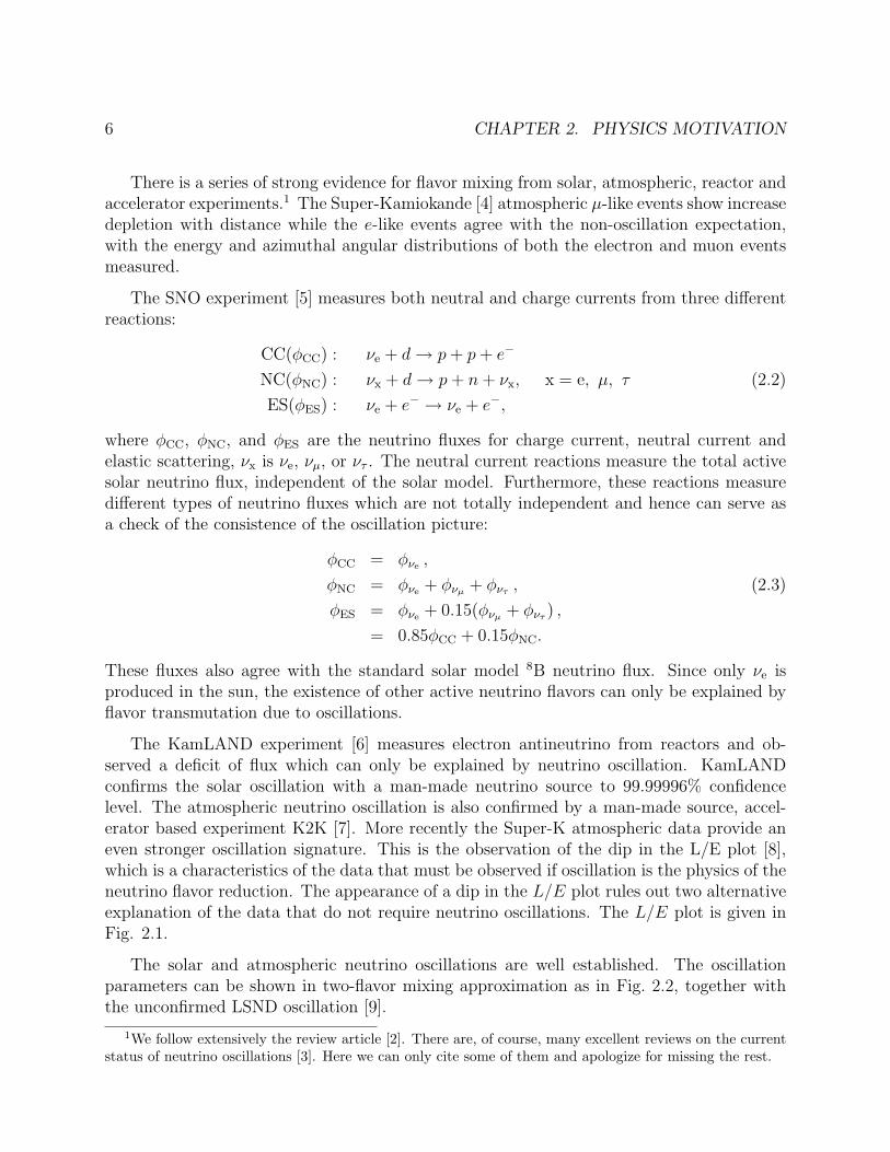
The KamLAND experiment [6] measures electron antineutrino from reactors and ob-served a deficit of flux which can only be explained by neutrino oscillation. KamLANDconfirms the solar oscillation with a man-made neutrino source to 99.99996% confidencelevel. The atmospheric neutrino oscillation is also confirmed by a man-made source, accel-erator based experiment K2K [7]. More recently the Super-K atmospheric data provide aneven stronger oscillation signature. This is the observation of the dip in the L/E plot [8],which is a characteristics of the data that must be observed if oscillation is the physics of theneutrino flavor reduction. The appearance of a dip in the L/E plot rules out two alternativeexplanation of the data that do not require neutrino oscillations. The L/E plot is given inFig. 2.1.
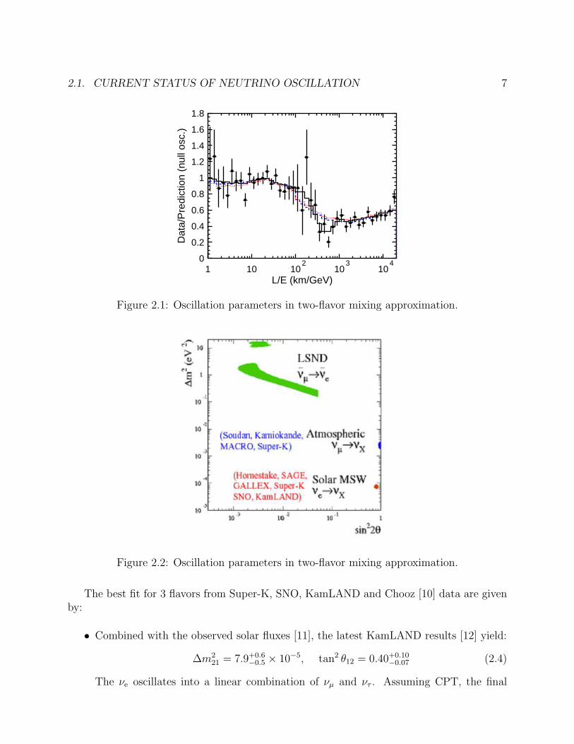
The solar and atmospheric neutrino oscillations are well established. The oscillationparameters can be shown in two-flavor mixing approximation as in Fig. 2.2, together withthe unconfirmed LSND oscillation [9].
1We follow extensively the review article [2]. There are, of course, many excellent reviews on the currentstatus of neutrino oscillations [3]. Here we can only cite some of them and apologize for missing the rest.
2.1. CURRENT STATUS OF NEUTRINO OSCILLATION 7
0
0.2
0.4
0.6
0.8
1
1.2
1.4
1.6
1.8
1 10 102
103
104 0
0.2
0.4
0.6
0.8
1
1.2
1.4
1.6
1.8
1 10 102
103
104
L/E (km/GeV)
Dat
a/P
redi
ctio
n (n
ull o
sc.)
Figure 2.1: Oscillation parameters in two-flavor mixing approximation.
Figure 2.2: Oscillation parameters in two-flavor mixing approximation.
The best fit for 3 flavors from Super-K, SNO, KamLAND and Chooz [10] data are givenby:
• Combined with the observed solar fluxes [11], the latest KamLAND results [12] yield:
∆m221 = 7.9+0.6
−0.5 × 10⁻⁵, tan2 θ12 = 0.40+0.10−0.07 (2.4)
The νe oscillates into a linear combination of νµ and ντ . Assuming CPT, the final
8 CHAPTER 2. PHYSICS MOTIVATION
confirmation of the LMA solution of the solar neutrino problem is provided by Kam-LAND [6] which has an average baseline to energy ratio near the second minimum ofthe survival probability νe → νe that is optimal for LMA. The KamLAND data excludeno oscillation at the 99.99996% C.L. and confirm the LMA solution by ruling out allother oscillation solutions, nonstandard neutrino interactions, and several other exoticscenarios [3]. Note that θ12 is 6σ away from being maximal2.
• The most recent SNO data obtained with salt added in the detector to improve sig-nificantly the efficiency of neutral current events detection, combined with the currentavailable data of solar neutrinos from Super-K, SNO, Homestake, Gallex and Sage,lead to [14, 15]:
∆m221 = 6.46× 10⁻⁵eV2, tan2 θ12 = 0.398 (2.5)
• Atmospheric [4]: The best fit gives [3]
|∆m232| = 2.1× 10⁻³eV2, sin2 2θ23 = 1.0. (2.6)
The allowed regions at 90% CL are
∆m232 = (1.5− 3.4)× 10−3eV2 (2.7)
sin2 2θ23 = 0.92− 1.0.
The dominant oscillation of atmospheric neutrinos is νµ → ντ .
• Chooz [10] reactor experiment:The Chooz experiment quoted the following bound for θ13:
sin2 2θ13 < 0.1 (θ13 < 9◦). (2.8)
The bounds extracted from the Chooz data is quite sensitive to the value of ∆m232
used. The more recent atmospheric oscillation data put a large bound on θ13. For∆m2
32 = 2.0× 10⁻³ eV2, sin2 2θ13 ≤ 0.2 at the 90% C.L., while for ∆m232 = 1.3× 10⁻³
eV2 the corresponding bound is 0.36 [3, 16].
• K2K long baseline accelerator experiment [17]:The K2K νµ survival measurement, the number of observed events and spectrum com-bined, is consistent with the atmospheric neutrino data. The Super-K and K2K com-bined fit gives ∆m2
32 = 2.0+0.4−0.3 × 10⁻³ eV2 [18].
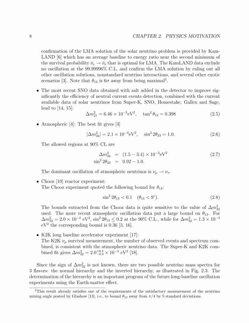
Since the sign of ∆m232 is not known, there are two possible neutrino mass spectra for
3 flavors: the normal hierarchy and the inverted hierarchy, as illustrated in Fig. 2.3. Thedetermination of the hierarchy is an important program of the future long-baseline oscillationexperiments using the Earth-matter effect.
2This result already satisfies one of the requirements of the satisfactory measurement of the neutrinomixing angle posted by Glashow [13], i.e., to bound θ12 away from π/4 by 5 standard deviations.
2.1. CURRENT STATUS OF NEUTRINO OSCILLATION 9
Figure 2.3: Normal and inverted spectra: normal ∆m232 > 0; inverted ∆m2
32 < 0.
There exists another set of neutrino oscillation data from the Los Alamos short baselinebeam-stop LSND experiment [9] which found evidence of the oscillation νµ → νe at thesignificance level of 3.3σ. The data require a mass square difference ∆m2 ≈ 0.2 − 1 eV2
and a very small mixing angle θLSND, sin2 2θLSND ≈ 0.003 − 0.04. The LSND collaborationalso observed the evidence of νµ → νe at lesser significance [19]. A large region allowed bythe LSND data has been ruled out by the KARMEN experiment [20], while the remainingallowed region will be tested by the MiniBooNE experiment in progress [21].
The LSND data can be interpreted by the existence of a sterile neutrino νs, or an anoma-lous muon decay µ+ → e+ + νe + νi, or a CPT violation effect which gives ν and ν differentmass spectra. But all are strongly disfavored [22].
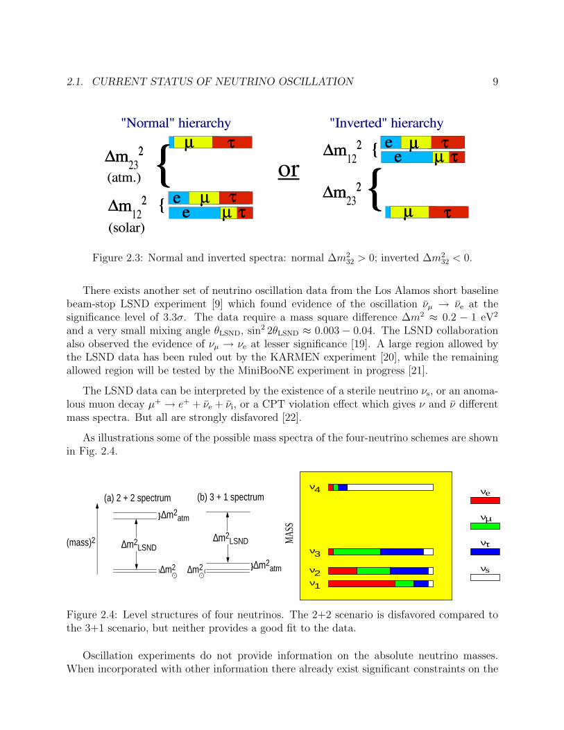
As illustrations some of the possible mass spectra of the four-neutrino schemes are shownin Fig. 2.4.
∆m2LSND
}
∆m2atm
(a) 2 + 2 spectrum
}
(b) 3 + 1 spectrum
∆m2LSND
}{
(mass)2
∆m2atm∆m2 ∆m2
ν
ν
ν
ν
ν
ν
ν
ν4
3
2
1
s
τ
µ
e
MAS
S
Figure 2.4: Level structures of four neutrinos. The 2+2 scenario is disfavored compared tothe 3+1 scenario, but neither provides a good fit to the data.
Oscillation experiments do not provide information on the absolute neutrino masses.When incorporated with other information there already exist significant constraints on the
10 CHAPTER 2. PHYSICS MOTIVATION
order of magnitude of the neutrino masses. This information comes from two sources. One isthe bound of the electron-neutrino mass from the study of the spectrum near the end pointof tritium decay. The other is from satellite-borne astrophysics experiments.
The most recent Mainz [23] and Troitsk [24] tritium experiments give mνe < 2.2 eV whichallows us to estimate the neutrino masses in two extreme cases in the 3-flavor scheme:
• Small mass scenario:Normal spectrum: m1 ≈ 0, m2 ≈ 0.008 eV, m3 ≈ 0.045 eV.Inverted spectrum: m3 ≈ 0, m1 ≈ 0.044 eV, m2 ≈ 0.045 eV.
• Large (degenerate) mass scenario:√∆m2
atm ≈ 0.045eV ¿ m1 ≈ m2 ≈ m3 < 2.2 eV
There also exists a cosmological bound on the sum of the masses of all stable neutrinosas provided by the most recent data on galaxy survey of the power spectrum of cosmicmicrowave background radiation from WMAP [25], 2dFGRS [26] and other measurements.The various fits give
∑
j
mνj< 0.42 ∼ 1.8 eV. (2.9)
This implies the following limit for the upper bound of the three neutrino scheme:
mν < 0.14 eV. (2.10)
Massive neutrinos are the first concrete evidence of physics beyond the standard modeland expose a hierarchy problem: the mass spectrum extends no less than 11 orders of mag-nitude: O(≤ 1 eV) − O(1011 eV). The very small mass and very large or even maximalmixing in the lepton sector, in contrast to the quark sector, seem to make the mass gener-ation mechanism in the standard model more chaotic. This casts doubts on how the Higgsmechanism can be a part of the fundamental structure of a fundamental theory.
For comparison we give the approximate mixing matrices for neutrino [27] [28]
UPMNS =
Ceiφ1 Seiφ2 S∗13
− Seiφ1/√
2 Ceiφ2/√
2 1/√
2
Seiφ1/√
2 − Ceiφ2/√
2 1/√
2
, (2.11)
where C = cos θ¯, S = sin θ¯ and S∗13 = sin θ13e−iδCP , and for quarks (in the Wolfenstein
form)
VCKM =
1− λ2/2 λ Aλ3(ρ− iη)−λ 1− λ2/2 Aλ2
Aλ3(1− ρ− iη) − Aλ2 1
, (2.12)
2.2. THEORETICAL EXPECTATIONS OF θ13 11
where A, ρ, η ∼ O(1) and λ ≈ 0.22. The lack of resemblance between the two mixingmatrices is clear. The generational hierarchical structure of the quark mixing is not shownin the leptonic sector. In the lepton sector the first and second generations have large mixing,the second and third probably have maximal mixing. The first and third has small mixing.It is important to know how small it is.
The large freedom in the construction of the neutrino mass matrix is subject to diversephysical interpretation. The most promising models of mν are the see-saw mechanism andZee model [29] of radiative masses; the see-saw mechanism requires Majorana neutrinos.
2.2 Theoretical expectations of θ13
Current experimental data, in particular those obtained from the Chooz [10] and Palo Verde[30] reactor neutrino experiments, yield an upper bound for θ13, θ13 < θC, where θC ≈ 13◦
which is the well-known Cabibbo angle in the quark flavor mixing. The smallness of θ13
requires a good theoretical explanation, which might simultaneously account for the largenessof θ12 and θ23. If θ13 = 0◦ held, there should exist a new flavor symmetry which forbids themixing between the first and third lepton families. In this special situation, in which themixing of 3 flavors can be understood in terms of 2-flavor mixing, there would be no leptonicCP and T violation to manifest in normal neutrino-neutrino and antineutrino-antineutrinooscillations.
A very challenging question is how small θ13 is, if it is not exactly zero. To answerthis question theoretically requires the knowledge of the origin of the fermion mass, flavormixing, and CP violation. In the absence of a reliable theory which provides the knowledge,we are unable to predict the value of θ13 model-independently. Nevertheless, it is possibleto obtain some useful information about the magnitude of θ13 phenomenologically from aglobal analysis of the known solar, atmospheric, reactor and accelerator neutrino oscillationdata [31, 32]. Such a “theoretical” expectation of θ13 may serve as a helpful guide to θ13
hunters to design a feasible experiment and maximize its range of sensitivity. In contrast, thevalues of θ13 predicted by the existing neutrino mass models depend more or less on some adhoc phenomenological assumptions [33]. Although the reliability of such model-dependentpredictions should not be overemphasized, some of them could shed light on the underlyingdynamics of lepton flavor mixing once θ13 is measured.
2.2.1 Expectations of θ13 from global three-neutrino analysis
In the scheme of three-flavor neutrino oscillations, a global analysis of the latest solar, at-mospheric, reactor (KamLAND and Chooz) and accelerator (K2K) neutrino data has beendone independently by Bahcall et al. (BGP) [31] and Maltoni et al. (MSTV) [32]. Becauseof the hierarchy ∆m2
sun ¿ ∆m2atm, it is a good approximation to neglect the effect of ∆m2
21
12 CHAPTER 2. PHYSICS MOTIVATION
in the analysis of atmospheric and K2K data, and to average out the effect of ∆m231 (or
∆m232) in the analysis of solar and KamLAND data. The Dirac-type CP-violating phase
is therefore decoupled from the global fit, and the analysis involves totally five parameters:θ12, θ23, θ13, ∆m2
21 and ∆m232). It is possible to obtain some helpful information about the
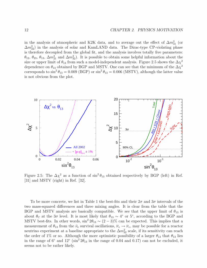
size or upper limit of θ13 from such a model-independent analysis. Figure 2.5 shows the ∆χ2
dependence on θ13 obtained by BGP and MSTV. One can see that the minimum of the ∆χ2
corresponds to sin2 θ13 = 0.009 (BGP) or sin2 θ13 = 0.006 (MSTV), although the latter valueis not obvious from the plot.
0
5
10
0 0.02 0.04 0.06
∆χ2 θ13vs
All 2002+ [p-p]ν-e ± 1%
∆χ2
sin2θ13
10 56789
10-2
10-1
sin2θ13
0
5
10
15
20
∆χ2
Atm
+ K
2K +
Cho
oz
Sol
ar +
Kam
LAN
D
Tot
al
Solar
Kam
LAN
D
3σ
90% CL
Figure 2.5: The ∆χ2 as a function of sin2 θ13 obtained respectively by BGP (left) in Ref.[31] and MSTV (right) in Ref. [32].
To be more concrete, we list in Table 1 the best-fits and their 2σ and 3σ intervals of thetwo mass-squared differences and three mixing angles. It is clear from the table that theBGP and MSTV analysis are basically compatible. We see that the upper limit of θ13 isabout θC at the 3σ level. It is most likely that θ13 ∼ 4◦ or 5◦, according to the BGP andMSTV best-fits. In other words, sin2 2θ13 ∼ (2− 3)% can be expected. This implies that ameasurement of θ13 from the νe survival oscillations, νe → νe, may be possible for a reactorneutrino experiment at a baseline appropriate to the ∆m2
32 scale, if its sensitivity can reachthe order of 1% or so. Although the more optimistic possibility of a larger θ13 that θ13 liesin the range of 6◦ and 12◦ (sin2 2θ13 in the range of 0.04 and 0.17) can not be excluded, itseems not to be rather likely.
2.2. THEORETICAL EXPECTATIONS OF θ13 13
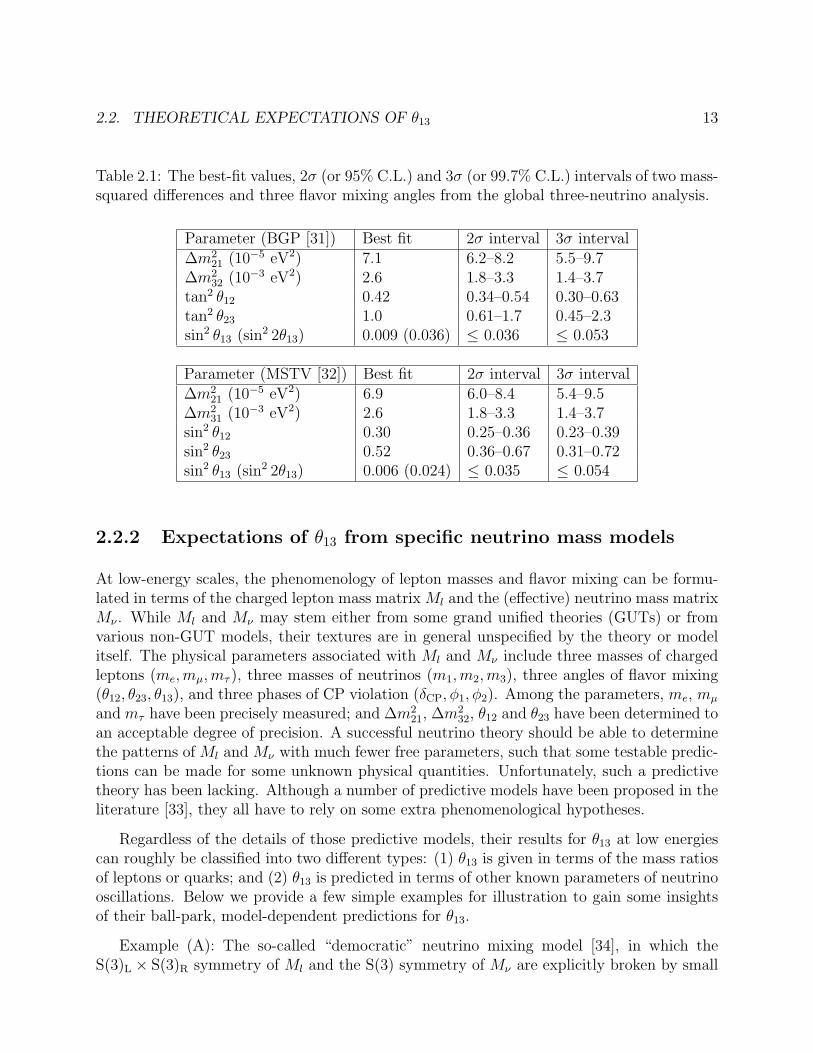
Table 2.1: The best-fit values, 2σ (or 95% C.L.) and 3σ (or 99.7% C.L.) intervals of two mass-squared differences and three flavor mixing angles from the global three-neutrino analysis.
Parameter (BGP [31]) Best fit 2σ interval 3σ interval∆m2
21 (10−5 eV2) 7.1 6.2–8.2 5.5–9.7∆m2
32 (10−3 eV2) 2.6 1.8–3.3 1.4–3.7tan2 θ12 0.42 0.34–0.54 0.30–0.63tan2 θ23 1.0 0.61–1.7 0.45–2.3sin2 θ13 (sin2 2θ13) 0.009 (0.036) ≤ 0.036 ≤ 0.053
Parameter (MSTV [32]) Best fit 2σ interval 3σ interval∆m2
21 (10−5 eV2) 6.9 6.0–8.4 5.4–9.5∆m2
31 (10−3 eV2) 2.6 1.8–3.3 1.4–3.7sin2 θ12 0.30 0.25–0.36 0.23–0.39sin2 θ23 0.52 0.36–0.67 0.31–0.72sin2 θ13 (sin2 2θ13) 0.006 (0.024) ≤ 0.035 ≤ 0.054
2.2.2 Expectations of θ13 from specific neutrino mass models
At low-energy scales, the phenomenology of lepton masses and flavor mixing can be formu-lated in terms of the charged lepton mass matrix Ml and the (effective) neutrino mass matrixMν . While Ml and Mν may stem either from some grand unified theories (GUTs) or fromvarious non-GUT models, their textures are in general unspecified by the theory or modelitself. The physical parameters associated with Ml and Mν include three masses of chargedleptons (me,mµ,mτ ), three masses of neutrinos (m1,m2,m3), three angles of flavor mixing(θ12, θ23, θ13), and three phases of CP violation (δCP, φ1, φ2). Among the parameters, me, mµ
and mτ have been precisely measured; and ∆m221, ∆m2
32, θ12 and θ23 have been determined toan acceptable degree of precision. A successful neutrino theory should be able to determinethe patterns of Ml and Mν with much fewer free parameters, such that some testable predic-tions can be made for some unknown physical quantities. Unfortunately, such a predictivetheory has been lacking. Although a number of predictive models have been proposed in theliterature [33], they all have to rely on some extra phenomenological hypotheses.
Regardless of the details of those predictive models, their results for θ13 at low energiescan roughly be classified into two different types: (1) θ13 is given in terms of the mass ratiosof leptons or quarks; and (2) θ13 is predicted in terms of other known parameters of neutrinooscillations. Below we provide a few simple examples for illustration to gain some insightsof their ball-park, model-dependent predictions for θ13.
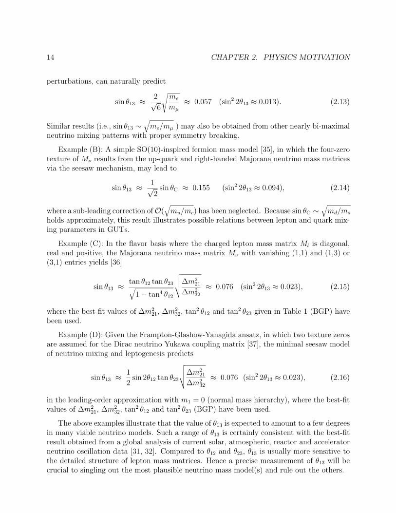
Example (A): The so-called “democratic” neutrino mixing model [34], in which theS(3)L × S(3)R symmetry of Ml and the S(3) symmetry of Mν are explicitly broken by small
14 CHAPTER 2. PHYSICS MOTIVATION
perturbations, can naturally predict
sin θ13 ≈ 2√6
√me
mµ
≈ 0.057 (sin2 2θ13 ≈ 0.013). (2.13)
Similar results (i.e., sin θ13 ∼√
me/mµ ) may also be obtained from other nearly bi-maximalneutrino mixing patterns with proper symmetry breaking.
Example (B): A simple SO(10)-inspired fermion mass model [35], in which the four-zerotexture of Mν results from the up-quark and right-handed Majorana neutrino mass matricesvia the seesaw mechanism, may lead to
sin θ13 ≈ 1√2
sin θC ≈ 0.155 (sin2 2θ13 ≈ 0.094), (2.14)
where a sub-leading correction ofO(√
mu/mc) has been neglected. Because sin θC ∼√
md/ms
holds approximately, this result illustrates possible relations between lepton and quark mix-ing parameters in GUTs.
Example (C): In the flavor basis where the charged lepton mass matrix Ml is diagonal,real and positive, the Majorana neutrino mass matrix Mν with vanishing (1,1) and (1,3) or(3,1) entries yields [36]
sin θ13 ≈ tan θ12 tan θ23√1− tan4 θ12
√√√√∆m221
∆m232
≈ 0.076 (sin2 2θ13 ≈ 0.023), (2.15)
where the best-fit values of ∆m221, ∆m2
32, tan2 θ12 and tan2 θ23 given in Table 1 (BGP) havebeen used.
Example (D): Given the Frampton-Glashow-Yanagida ansatz, in which two texture zerosare assumed for the Dirac neutrino Yukawa coupling matrix [37], the minimal seesaw modelof neutrino mixing and leptogenesis predicts
sin θ13 ≈ 1
2sin 2θ12 tan θ23
√√√√∆m221
∆m232
≈ 0.076 (sin2 2θ13 ≈ 0.023), (2.16)
in the leading-order approximation with m1 = 0 (normal mass hierarchy), where the best-fitvalues of ∆m2
21, ∆m232, tan2 θ12 and tan2 θ23 (BGP) have been used.
The above examples illustrate that the value of θ13 is expected to amount to a few degreesin many viable neutrino models. Such a range of θ13 is certainly consistent with the best-fitresult obtained from a global analysis of current solar, atmospheric, reactor and acceleratorneutrino oscillation data [31, 32]. Compared to θ12 and θ23, θ13 is usually more sensitive tothe detailed structure of lepton mass matrices. Hence a precise measurement of θ13 will becrucial to singling out the most plausible neutrino mass model(s) and rule out the others.
2.3. MEASUREMENT OF θ13 15
2.3 Measurement of θ13
The oscillatory effect of the mixing angle θ13 is generally subleading or small. The effectshows either in the high energy (order of GeV) νe(νe) → νe(νe) survival processes or theνµ(νµ) → νe(νe) low energy (order of MeV) appearance processes. The latter are performedat accelerator based long baseline experiments and the former short distance reactor experi-ments. Because of the limited flux intensity of neutrino beams currently available and thoseplanned for the near future, and also because of the inherent complications, the accuracy of-fered by long baseline accelerator experiments in the near future is limited, probing sin2 2θ13
in the region no lower than 0.4, while reactor experiments have a much better precision inthe 0.01 range which can be obtained before the end of this decade. We discuss and providea short overview of the two types of experiments below.
2.3.1 Long-baseline experiments and the measurement θ13
In the near term, the first generation accelerator based long-baseline experiments with con-ventional νµ beams, K2K, MINOS, and OPERA/ICARUS, should be able to confirm atmo-spheric neutrino oscillations and improve the precision with which ∆m2
32 and sin2 2θ23 aredetermined. Experiments that measure νµ disappearance will establish the first minimumin the νµ → νµ oscillation. The K2K experiment from KEK to Super-K [17], a distance ofL = 250 km, has begun taking data again following the restoration of the Super-K detector.To date K2K has confirmed neutrino oscillation to the 3.9σ level. The MINOS experimentfrom Fermilab to the Soudan mine [38], at a distance of L = 730 km, has been commencedon March 4, 2005 when the first neutrino beam from Fermilab main injector was provided[39]; it is expected to obtain 10% precision on ∆m2
32 and sin2 2θ23 in 3 years running. TheCERN to Gran Sasso (CNGS) experiments, ICARUS [40] and OPERA [41], also at a dis-tance L = 730 km but with higher neutrino energy, are expected to be online in mid 2006.The appearance of ντ should be observed in the CNGS experiments, which would confirmthat the primary oscillation of atmospheric neutrinos is νµ → ντ . These European programswould also contribute to obtaining a better limit for θ13.
The three parameters that are not determined by the solar, atmospheric, and KamLANDdata are θ13 which is crucial for the Dirac CP effect, the sign of ∆m2
32 which fixes thehierarchy of neutrino masses, and the Dirac CP phase δCP . The appearance of νe in νµ → νe
oscillations is the most critical measurement, since the probability is proportional to sin2 2θ13
in the leading oscillation, for which there is currently only an upper bound (0.1 at the90% C. L., from the Chooz [10] and Palo Verde [30] reactor experiments). By combiningICARUS/MINOS/OPERA data, it may be possible to establish whether sin2 2θ13 > 0.01 at90% C. L. [42]. With OPERA and ICARUS the accuracy of the measurement of sin2 2θ13 isexpected to be a lower limit of 0.06-0.04. A summary of the status of the near term programsup to August 2004 can be found in [43].
16 CHAPTER 2. PHYSICS MOTIVATION
In the longer term the focus shifts primarily to νµ → νe oscillations performed at ac-celerator based long baseline experiments. A measurement of both νµ → νe and νµ → νe
oscillations allows one to measure θ13 and test for CP violation in the lepton sector, providedthat θ13 is large enough. However, there are difficulties coming from different aspects of suchexperiments that must be overcome, in addition to the fact νµ → νe oscillation is subdom-inant. One of the difficulties is the significant background coming from three sources [44]:(a) the νe contamination in the νµ beam; (b) decay of ντ → νe when τ is produced from thedominant oscillation νν → ντ ; (c) background for the detection of e events in calorimetricdetectors.
Another difficulty, which is inherent in the theoretical formulation, is known as parameterdegeneracies that occur when two or more parameter sets are consistent with the same data.The degeneracies in general lead to ambiguities in the measured values of θ13 and δCP evenif the oscillation probabilities νµ → νe and νµ → νe are precisely known [45, 46]. There arepotentially three two-fold parameter degeneracies: (i) the (δCP , θ13) ambiguity [45, 47, 48,49, 50], (ii) the ambiguity due to our lack of knowledge of the mass hierarchy (the sign of∆m2
32 ambiguity) [45, 48, 51, 52], and (iii) the (θ23,π2− θ23) ambiguity [45, 58], which occurs
because only sin2 2θ23, not θ23, is measured in atmospheric neutrino experiments. Each setof the parameter degeneracies can lead to different inferred values for δCP and θ13, and thethree sets can all be present simultaneously, leading to as much as an eight-fold ambiguitiesin the determination of θ13 and δCP . In many cases both CP conserving and CP violatingparameter sets are allowed by the same data because of the degeneracies.
Still another problem is that Earth-matter effects can induce fake CP violation, whichmust be taken into account in any determination of θ13 and δCP in long baseline experiments.One advantage of matter effects is that they might distinguish between the two possible masshierarchies.
The future precision measurements will rely on two types of new facilities: the superbeam[53] and the neutrino factory [54]. The high neutrino flux of the superbeam, such as theJ-PARC [55] under construction, and other facilities under planning, such as NuMI off-axisNOνA [56] at FNAL and the off-axis program of Brookhaven Wide Band Beam [57], will goa long way to pin down fairly accurately most of the oscillation parameters, including theDirac CP phase. The J-PARC neutrino program will not begin before 2009 and the FermilabNOνA and BNL Wide Band Beam programs are still in the stage of feasibility study.
The neutrino factory will be the ultimate facility to study neutrino oscillations. Withsuch a facility the very accurate measurement of neutrino oscillation parameters, the studyof appearance channels, and the investigation the CPT invariance can be carried out.
2.3. MEASUREMENT OF θ13 17
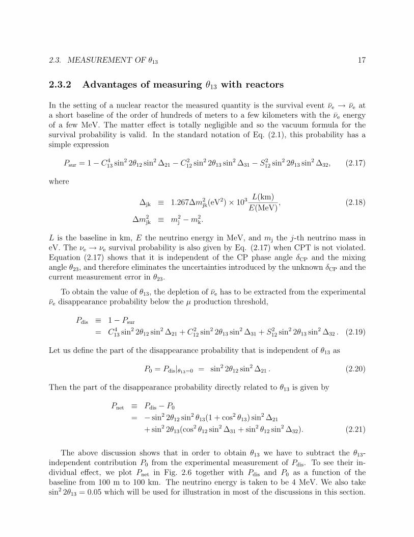
2.3.2 Advantages of measuring θ13 with reactors
In the setting of a nuclear reactor the measured quantity is the survival event νe → νe ata short baseline of the order of hundreds of meters to a few kilometers with the νe energyof a few MeV. The matter effect is totally negligible and so the vacuum formula for thesurvival probability is valid. In the standard notation of Eq. (2.1), this probability has asimple expression
Psur = 1− C413 sin2 2θ12 sin2 ∆21 − C2
12 sin2 2θ13 sin2 ∆31 − S212 sin2 2θ13 sin2 ∆32, (2.17)
where
∆jk ≡ 1.267∆m2jk(eV
2)× 103 L(km)
E(MeV), (2.18)
∆m2jk ≡ m2
j −m2k.
L is the baseline in km, E the neutrino energy in MeV, and mj the j-th neutrino mass ineV. The νe → νe survival probability is also given by Eq. (2.17) when CPT is not violated.Equation (2.17) shows that it is independent of the CP phase angle δCP and the mixingangle θ23, and therefore eliminates the uncertainties introduced by the unknown δCP and thecurrent measurement error in θ23.
To obtain the value of θ13, the depletion of νe has to be extracted from the experimentalνe disappearance probability below the µ production threshold,
Pdis ≡ 1− Psur
= C413 sin2 2θ12 sin2 ∆21 + C2
12 sin2 2θ13 sin2 ∆31 + S212 sin2 2θ13 sin2 ∆32 . (2.19)
Let us define the part of the disappearance probability that is independent of θ13 as
P0 = Pdis|θ13=0 = sin2 2θ12 sin2 ∆21 . (2.20)
Then the part of the disappearance probability directly related to θ13 is given by
Pnet ≡ Pdis − P0
= − sin2 2θ12 sin2 θ13(1 + cos2 θ13) sin2 ∆21
+ sin2 2θ13(cos2 θ12 sin2 ∆31 + sin2 θ12 sin2 ∆32). (2.21)
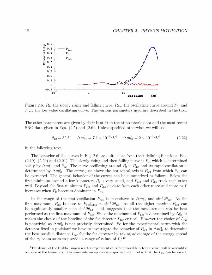
The above discussion shows that in order to obtain θ13 we have to subtract the θ13-independent contribution P0 from the experimental measurement of Pdis. To see their in-dividual effect, we plot Pnet in Fig. 2.6 together with Pdis and P0 as a function of thebaseline from 100 m to 100 km. The neutrino energy is taken to be 4 MeV. We also takesin2 2θ13 = 0.05 which will be used for illustration in most of the discussions in this section.
18 CHAPTER 2. PHYSICS MOTIVATION
-0.1
0
0.1
0.2
0.3
0.4
0.5
0.6
0.7
0.8
0.9
10-1
1 10
PdisP0Pnet
Baseline (km)
Probability
Figure 2.6: P0: the slowly rising and falling curve, Pdis: the oscillating curve around P0, andPnet: the low value oscillating curve. The various parameters used are described in the text.
The other parameters are given by their best fit in the atmospheric data and the most recentSNO data given in Eqs. (2.5) and (2.6). Unless specified otherwise, we will use
θ12 = 32.5◦, ∆m221 = 7.1× 10⁻⁵eV2, ∆m2
31 = 2× 10⁻³eV2 (2.22)
in the following text.
The behavior of the curves in Fig. 2.6 are quite clear from their defining functions, Eqs.(2.19), (2.20) and (2.21). The slowly rising and then falling curve is P0, which is determinedsolely by ∆m2
21 and θ12. The curve oscillating around P0 is Pdis and its rapid oscillation isdetermined by ∆m2
32. The curve just above the horizontal axis is Pnet from which θ13 canbe extracted. The general behavior of the curves can be summarized as follows: Below thefirst minimum around a few kilometers P0 is very small, and Pnet and Pdis track each otherwell. Beyond the first minimum Pnet and Pdis deviate from each other more and more as Lincreases when P0 becomes dominant in Pdis.
In the range of the first oscillation Pnet is insensitive to ∆m221 and sin2 2θ12. At the
first maximum, Pdis is close to Pnet|Max ' sin2 2θ13. At all the higher maxima Pnet canbe significantly smaller than sin2 2θ13. This suggests that the measurement can be bestperformed at the first maximum of Pnet. Since the maximum of Pnet is determined by ∆2
32, itmakes the choice of the baseline of the far detector Lfar critical. However the choice of Lfar
is nontrivial as ∆m232 is not precisely determined. So for the experimental setup with the
detector fixed in position3 we have to investigate the behavior of Pnet in ∆m232 to determine
the best possible distance Lfar for the far detector by taking advantage of the energy spreadof the νe beam so as to provide a range of values of L/E.
3The design of the Diablo Canyon reactor experiment calls for a movable detector which will be assembledout side of the tunnel and then move into an appropriate spot in the tunnel so that the Lfar can be varied.
2.3. MEASUREMENT OF θ13 19
In the case that the incident neutrino energy can be determined event by event, as isthe case of reactor experiments, a range of values of L/E is provided by the neutrino beamenergy spectrum which will be very helpful in the determination of θ13, although a largeamount of statistics is required.
The νe interaction rate depends on its flux and the cross section of inverse beta decayνe+p → n+e+ [59]. The quasi elastic cross section is given in [60] and the phenomenologicalνe flux can be found in [61]. For the present discussion the shape of the interaction rate whichdepends on the neutrino energy is needed, while the normalization of the interaction ratewhich depends on the baseline is unimportant. Up to a normalization factor, the interactionrate without oscillation can be approximately expressed as
(dN
dE
)
NO
∼ exp(a0 + a1E + a2E2)(E − 1.293MeV)
√(E − 1.293MeV)2 −m2
e, (2.23)
where the energy of neutrino E is in MeV, a0=4.509, a1=-0.2171 MeV−1, a2=-0.08880 MeV−2,(E − 1.293 MeV) is the energy of the positron, and me is the mass of the positron in MeV.The interaction rate in the presence of oscillation is
(dN
dE
)
OSC
=
(dN
dE
)
NO
Psur, (2.24)
where Psur is given by Eq. (2.17). Further discussion on neutrino energy spectrum can befound in the next chapter.
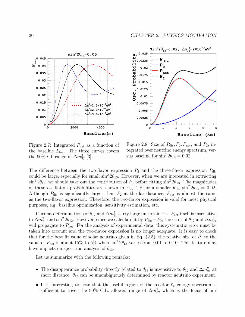
To demonstrate the critical nature of Lfar, we weight Pnet by interaction rate and integrateover the whole neutrino energy spectrum. The integrated Pnet is plotted in Fig. 2.7 as afunction of Lfar for three values of ∆m2
32, i.e., (1.3, 2.0, 3.0) × 10−3 eV2, which cover the∆m2
32 allowed range in the 90% CL [3]. sin2 2θ13 is taken to be 0.05. Curves of other valuesof sin2 2θ13 scale identically to those of Fig. 2.7. The curves show that Pnet is sensitiveto ∆m2
32 and varies significantly in the presently allowed range of its value. The maximalprobabilities in this range of ∆m2
32 cover a sizable region of Lfar from 1.5 to 3.5 km. For∆m2
32 = (1.3, 2.0, 3.0)×10−3 eV2, the oscillation maxima correspond to a baseline of 3500m,2200m, and 1500m, respectively. Furthermore, a maximum for ∆m2
32 = 1.3 × 10⁻³ eV2 isnear a minimum of ∆m2
32 = 3.0 × 10⁻³ eV2. These features can create complications andtherefore indicate the challenge in the selection of the baseline of the far detector, Lfar. Fromthis simply study, placing the far detector at 1800 m to 2200 m from the reactor looks to bea good choice. In addition, statistics must be taken into consideration in the choice of Lfar
as the event rate is proportional to 1/L2far. Detailed baseline optimization with statistical
and systematic errors, backgrounds, and concrete geographical condition taken into accountwill be discussed later.
In the literature, a simplified expression for oscillation probability involving only 2 neu-trino flavors is often used for describing reactor neutrino experiment at short distance:
P2 = sin2 2θ13 sin2 ∆31 . (2.25)
20 CHAPTER 2. PHYSICS MOTIVATION
0
0.005
0.01
0.015
0.02
0.025
0.03
0.035
0.04
0.045
0 2000 4000
sin22θ13=0.05
∆m2=1.3×10⁻³eV2
Baseline(m)
Pnet
∆m2=2.0×10⁻³eV2
∆m2=3.0×10⁻³eV2
Figure 2.7: Integrated Pnet as a function ofthe baseline Lfar. The three curves coversthe 90% CL range in ∆m2
32 [3].
0
0.0025
0.005
0.0075
0.01
0.0125
0.015
0.0175
0.02
0.0225
0.025
0 1 2 3 4 5
Sin22θ13=0.02, ∆m312=2×10⁻³eV2
PdisP0PnetP2
Baseline (km)Osc. Probability
Figure 2.8: Size of Pdis, P0, Pnet, and P2, in-tegrated over neutrino energy spectrum, ver-sus baseline for sin2 2θ13 = 0.02.
The difference between the two-flavor expression P2 and the three-flavor expression Pdis
could be large, especially for small sin2 2θ13. However, when we are interested in extractingsin2 2θ13, we should take out the contribution of P0 before fitting sin2 2θ13. The magnitudesof these oscillation probabilities are shown in Fig. 2.8 for a smaller θ13, sin2 2θ13 = 0.02.Although Pdis is significantly larger than P2 at the far distance, Pnet is almost the sameas the two-flavor expression. Therefore, the two-flavor expression is valid for most physicalpurposes, e.g. baseline optimization, sensitivity estimation, etc.
Current determinations of θ12 and ∆m221 carry large uncertainties. Pnet itself is insensitive
to ∆m221 and sin2 2θ12. However, since we calculate it by Pdis−P0, the error of θ12 and ∆m2
21
will propagate to Pnet. For the analysis of experimental data, this systematic error must betaken into account and the two-flavor expression is no longer adequate. It is easy to checkthat for the best fit value of solar neutrino given in Eq. (2.5), the relative size of P0 to thevalue of Pnet is about 15% to 5% when sin2 2θ13 varies from 0.01 to 0.10. This feature mayhave impacts on spectrum analysis of θ13.
Let us summarize with the following remarks:
• The disappearance probability directly related to θ13 is insensitive to θ12 and ∆m221 at
short distance. θ13 can be unambiguously determined by reactor neutrino experiment.
• It is interesting to note that the useful region of the reactor νe energy spectrum issufficient to cover the 90% C.L. allowed range of ∆m2
32 which is the focus of our
2.3. MEASUREMENT OF θ13 21
discussion. And we determine that the optimal choice of Lfar to be 1800m to 2200m.
• The disappearance probability is sensitive to ∆m231. On one side, it creates challenge
in the selection of baseline of the far detector. On the other side, the wide neutrinoenergy spectrum will provide information of ∆m2
31.
• The simplified two-flavor oscillation expression is a very good approximation of thethree-flavor expression, except that errors of θ12 and ∆m2
21 can not be taken intoaccount in the former. These systematic errors may have a significant impact on thedata analysis.
Finally, we conclude from this theoretical investigation that the choice of Lfar be madeso that it can cover as large a range of ∆m2
32 as possible.
Bibliography
[1] Z. Maki, Nakagawa, and S. Sakata, Prog. Theor. Phys. 28, 870 (1962); B. Pontecorvo,Sov. Phys. JETP 26, 984 (1968), V.N. Gribov and B. Pontecorvo, Phys. Lett. 28B, 493(1969).
[2] Y. Wang, Plenary talk given at the ”32nd International Conference on High EnergyPhysics”, Aug. 16-22, 2004, Beijing, China [arXiv:hep-ex/0411028].
[3] V. Barger, D. Marfatia, and K. Whisnant, Int. J. Mod. Phys. E 12, 569 (2003)[arXiv:hep-ph/0308123]. A. Smirnov, Neutrino Physics after KamLAND, Invited talkat the 4th Neutrino Oscillations and their Oringin (NOON 2003), Kanazawa, Japan,Feb. 10-14, 2003, [arXiv:hep-ph/0306075]; J.W.F. Valle, Neutrino mass twenty-fiveyears later, AIP Conf. Proc. 687 16 (2003), [arXiv:hep-ph/0307192]; B. Kayser, Neu-trino Physics: Where Do We Stand, and Where are We Going?–The Theoretical andPhenomenological Perspective [arXiv:hep-ph/0306072], in Review of Particle Physics2002 [27]. Z.-Z. Xing, Flavor Mixing and CP Violation of Massive Neutrinos, Int. J.Mod. Phys. A19, 1 (2004) [arXiv:hep-ph/0307359].
[4] SuperK Collaboration (atmospheric) Y. Fukuda et al., Phys. Lett. B433, 9 (1998)[arXiv:hep-ex/9803006]; Phys. Rev. Lett., 81, 1562 (1998) [arXiv:9807003]; 82, 2644(1999) [arXiv:hep-ex/9812014]; Phys Lett. B467, 185 (1999) [arXiv:hep-ex/9908049].
[5] SNO Collaboration: Q.R. Ahmad et al., Phys. Rev. Lett. 87, 071301 (2001) (arXiv:nucl-ex/0106015); 89, 011301 (2002) [arXiv:nucl-ex/0204008]; 89, 011302 (2002) [arXiv:nucl-ex/0204009].
[6] KamLAND Collaboration: K. Eguchi et al., Phys. Rev. Lett., 90 021802 (2003)[arXiv:hep-ex/0212021].
[7] K2K collaboration, M.H. Ahn et al, Phys. Rev. Lett. 93 051801 (2004). [arXiv:hep-ex/0402017]
[8] Super-K Collaboration (L/E data): Y. Ashie et al., Evidence for an oscilatory signaturein atmospheric oscillation, Phys. Rev. Lett. 93, 101801 (2004) [arXiv:hep-ex/0404034].
22
BIBLIOGRAPHY 23
[9] LSND Collaboration (νµ → νe): C. Athanassopoulos et al., Phys. Rev. C54, 2685 (1996)[arXiv:hep-ex/9605001]; Phys. Rev. Lett. 77 3082 (1996) [arXiv:hep-ex/9605003]; A.Aguilar et al., Phys. Rev. D64 112007 (2001) [arXiv:hep-ex/0104049].
[10] M. Apollonio et al. [Chooz Collaboration], Phys. Lett. B 420 397 (1998) [arXiv:hep-ex/9711002]; Phys. Lett. B 466 415 (1999) [arXiv:hep-ex/9907037]; Eur. Phys. J. C 27331 (2003) [arXiv:hep-ex/0301017].
[11] SuperK Collaboration (solar): Y. Fukuda et al., Phys. Rev. Lett., 82, 1810 and2430 (1999); 86, 5651 (2001) [arXiv:hep-ex/010302]; Phys. Lett. B539, 179 (2002)[arXiv:hep-ex/0205075]; M.B. Smy et al., Phys. Rev. D69, 011104 (2004) [arXiv:hep-ex/0309011].
[12] KamLAND Collaboration: T. Araki et al., Phys. Rev. Lett. 94, 081801 (2005)[arXiv:hep-ex/0406035].
[13] S.L. Glashow, Fact & Fancy in Neutrino Physics II, Talk at the 10th International Work-shop on Neutrino Telescope, Venice, Italy, March 11-14, 2003 arXiv:hep-ph/0306100.
[14] SNO Collaboration (salt added): A. Ahmed et al., Phys. Rev. Lett. 92 181301 (2004).
[15] M. Maltoni, T. Schwetz, M.A. Tortola, and J.W.F. Valle, Status of three-neutrino os-cillations after the SNO-salt data, Phys. Rev. D68, 113010 (2003) [hep-ph/0309130].
[16] SuperK Collaboration: T. Nakaya, eConf. (2002) C0206620, SAAT01 [arXiv:hep-ex/0209036].
[17] K2K Collaboration S. H. Ahn et al., Phys. Lett. B 511, 178 (2001) [arXiv:hep-ex/0103001]; Phys. Rev. Lett. 90, 041801 (2003) [arXiv:hep-ex/0212007].
[18] G.L. Fogli, E. Lisi, A. Marrone, D. Montanino, A. Palazzo, and A.M. Rotunno, Phys.Rev. D69, 017301 (2004) [arXiv: hep-ph/0308055].
[19] LSND Collaboration (νµ → νe): C. Athanassopoulos et al., Phys. Rev. C58, 2489 (1998)[arXiv:hep-ex/9706006]; Phys. Rev. Lett. 81, 1774 (1998) [arXiv:hep-ex/9709006].
[20] KARMEN Collaboration: K. Eitel et al., Nucl. Phys. Proc. Suppl. 91 191 (2000)[arXiv:hep-ex/0008002]; B. Armbruster et al., Phys. Rev. D66, 112001 (2002)[arXiv:hep-ex/0203021].
[21] MiniBooNE Collaboration: I. Stancu et al., FERMILAB-TM-2207.
[22] M. Maltoni, T. Schwetz, M.A. Tortola, and J.W. Valle, Nucl. Phys. B643, 321 (2002)[arXiv:hep-ph/0207157].
[23] Mainz: C. Weinheimer et al., Phys. Lett. B460, 219 (1999).
24 BIBLIOGRAPHY
[24] Troitsk: V.M. Lobshev et al., Phys. Lett. B460, 227 (1999).
[25] WMAP Collaboration: D Spergel et al., Astrophys. J. Suppl. 148, 175 (2003)[arXiv:astro-ph/0302209]
[26] 2dFGRS Collaboration: M. Colless et al., Mon. Not. Roy. Aston. Soc. 328, 1039 (2001)[arXiv:astro-ph/0106498].
[27] The Particle Data Group: K. Hagiwara et al. Phys. Rev. D66, 010001 (2002).
[28] B. Kayser, appeared in [27] P. 392.
[29] A. Zee, Phys. Lett. 93, 389 (1980); K. Babu, Phys. Lett. 203, 132 (1988).
[30] F. Boehm et al., Phys. Rev. Lett. 84, 3764 (2000) [arXiv:hep-ex/9912050]; Phys. Rev. D62, 072002 (2000) [arXiv:hep-ex/0003022]; Phys. Rev. D 64, 112001 (2001) [arXiv:hep-ex/0107009].
[31] J.N. Bahcall and C. Pena-Garay, JHEP 0311, 004 (2003); see also, M.C. Gonzalez-Garcia and C. Pena-Garay, Phys. Rev. D 68, 093003 (2003).
[32] M. Maltoni, T. Schwetz, M.A. Tortola, and J.W.F. Valle, New J. Phys. 6, 122 (2004)[arXiv:hep-ph/0405172].
[33] For recent reviews with extensive references, see: H. Fritzsch and Z.Z. Xing, Prog.Part. Nucl. Phys. 45, 1 (2000); R.N. Mohapatra, talk at Conference on Physics Be-yond the Standard Model: Beyond the Desert 02, Oulu, Finland, 2-7 Jun 2002, andat 10th International Conference on Supersymmetry and Unification of FundamentalInteractions (SUSY02), Hamburg, Germany, 17-23 Jun 2002. hep-ph/0211252; M.C.Gonzalez-Garcia and Y. Nir, Rev. Mod. Phys. 75, 345 (2003); G. Altarelli and F. Fer-uglio, talk at the 10th International Workshop on Neutrino Telescopes, Venice, Italy,11-14 Mar 2003, hep-ph/0306265; S.F. King, Rept Prog. Phys. 67, 107 (2004) [hep-ph/0310204]; V. Barger, D. Marfatia, and K. Whisnant, Int. J. Mod. Phys. E 12, 569(2003); Z.Z. Xing, the last article in Ref. [3].
[34] H. Fritzsch and Z.Z. Xing, Phys. Lett. B 372, 265 (1996).
[35] W. Buchmuller and D. Wyler, Phys. Lett. B 521, 291 (2001).
[36] P.H. Frampton, S.L. Glashow, and D. Marfatia, Phys. Lett. B 536, 79 (2002).
[37] P.H. Frampton, S.L. Glashow, and T. Yanagida, Phys. Lett. B 548, 119 (2002).
[38] MINOS Collaboration, Fermilab Report No. NuMI-L-375 (1998).
BIBLIOGRAPHY 25
[39] MINOS Collaboration: See Fermilab news release at:http://www.fnal.gov/pub/presspass/press releases/minos dedication 3-4-05.html. Fora most recent overview of the status of MINOS, see B. Rebel,talk given in Frontiersin Contemporay Physics III, May 23-28, 2005, http://www.fcp05.vanderbilt.edu/; K.Grzelak, LBL Experiments in the US talk at the it Neutrino Oscillation Workshop 2004(NOW2004), September 11-17, 2004, Otranto, Italy.
[40] ICARUS Collaboration: A. Rubbia, Status Of The Icarus Experiment, talk at Skandi-navian Neutrino Workshop (SNOW), Uppsala, Sweden, February 2001, Phys. ScriptaT93, 70 (2001); F.Ronga, LBL Experiments in Europe, talk at the Neutrino OscillationWorkshop 2004 (NOW2004), September 11-17, 2004, Otranto, Italy.
[41] OPERA Collaboration, CERN/SPSC 2000-028, SPSC/P318, LNGS P25/2000, July,2000; F.Ronga, LBL Experiments in Europe, talk at the Neutrino Oscillation Workshop2004 (NOW2004), September 11-17, 2004, Otranto, Italy.
[42] V. D. Barger, A. M. Gago, D. Marfatia, W. J. Teves, B. P. Wood and R. ZukanovichFunchal, Phys. Rev. D 65, 053016 (2002) [arXiv:hep-ph/0110393].
[43] Stephane T’Jampens, Current and near future long baseline experiments, talk give atthe 6th Internation Workshop on Neurino Factories and Superbeams, July 23-Aug. 1,2004, Osaka University, Osaka, Japan (http://www-kuno.phys.sci.osaka-u.ac.jp/ nu-fact04/agenda.html).
[44] M. Goodman, Plans for Experiments to Measure θ13, talk given at the Coral GablesConference on Lauching of Belle Epoque in High-Energy Physics and Cosmology (CG2003), Ft. Lauiderdale, Florida, 17-21 December 2003; arXiv:hep-ex/0404031.
[45] V. Barger, D. Marfatia and K. Whisnant, Phys. Rev. D 65, 073023 (2002) [arXiv:hep-ph/0112119].
[46] H. Minakata, H. Nunokawa and S. Parke, Phys. Rev. D 66, 093012 (2002) [arXiv:hep-ph/0208163].
[47] J. Burguet-Castell, M. B. Gavela, J. J. Gomez-Cadenas, P. Hernandez and O. Mena,Nucl. Phys. B 608, 301 (2001) [arXiv:hep-ph/0103258].
[48] V. D. Barger, D. Marfatia and K. Whisnant, in Proc. of the APS/DPF/DPB SummerStudy on the Future of Particle Physics (Snowmass 2001), ed. N. Graf, eConf C010630,E102 (2001) [arXiv:hep-ph/0108090].
[49] T. Kajita, H. Minakata, and H. Nunokawa, Phys. Lett. B528, 245 (2002) [arXiv:hep-ph/0112345].
[50] P. Huber, M. Lindner, and W. Winter, Nucl. Phys. B645, 3 (2002) [arXiv:hep-ph/0204352].
26 BIBLIOGRAPHY
[51] P. Lipari, Phys. Rev. D 61, 113004 (2000) [arXiv:hep-ph/9903481]; I. Mocioiu andR. Shrock, Phys. Rev. D 62, 053017 (2000) [arXiv:hep-ph/0002149]; V. D. Barger,S. Geer, R. Raja and K. Whisnant, Phys. Lett. B 485, 379 (2000) [arXiv:hep-ph/0004208]; M. Koike, T. Ota and J. Sato, Phys. Rev. D 65, 053015 (2002) [arXiv:hep-ph/0011387]; H. Minakata and H. Nunokawa, JHEP 0110, 001 (2001) [arXiv:hep-ph/0108085].
[52] V. D. Barger, S. Geer, R. Raja and K. Whisnant, Phys. Rev. D 62, 013004 (2000)[arXiv:hep-ph/9911524].
[53] B. Richter, Conventional beams or neutrino factoies, arXiv:hep-ph/0008222; K. Dydak,talk at NOW2000; D. Harris, Superbeams, talk given at NuFact 04, Osaka, Japan;M. Messetto, (European Ideas on) Super Beams (and Beta Beams), talk given at theNeutrino Oscillation Workshop 2004 (NOW2004), September 11-17, 2004, Otranto,Italy.
[54] D.G. Koshkarev, CERN internal report CERN/ISR-DI/74 (1974); S. Geer Phys. Rev.D57, 6989 (1998); A. Blondel et al., Nucl. Instrum. Meth. A451, 102 (2000); M. Lind-ner, Oscillation neutino physics reach at neutrino factories, talk given at NuFact 04,Osaka, Japan; R. Edgecock, Neutrino factory R&D in Europe, talk given at NuFact 04,Osaka, Japan; Derun Li, Neutrino factory R&D in the U.S., talk given at NuFact 04,Osaka, Japan.
[55] Y. Ito et al.,The JHF-Kamioka neutrino project, in Neutino Oscillation and Their Ori-gins (NOON2001), Deceemberr 5-8, 2001, Kashiwa, Japan; K. Kaneyuki, T2K exper-iment, current status and physics sensitivity, talk given at the Neutrino OscillationWorkshop 2004 (NOW2004), September 11-17, 2004, Otranto, Italy.
[56] D. Ayres et al., Letter of intend to build an off-axis detector to study the νµ → νe withthe NuMI neutrino beam, arXiv:hep-ex/0210005; P. Litchfield, NOνA, talk given atthe Neutrino Oscillation Workshop 2004 (NOW2004), September 11-17, 2004, Otranto,Italy; O. Mena Requejo, S. Palomnares-Ruiz, and S. Pascoli, Super-NOνA: a long-baseline neutrino experiment with two off-axis detectors, arXiv:hep-ph/0504015.
[57] M. Diwan et al., Report of the BNL Neutrino Working Group: Very long baselineneutrino oscillation experiment for precise determination of oscillation paramenters andsearch for νµ → νe appearance and CP violation, arXiv:hep-ex/0211001; Very longbaseline neutrino oscillation experiment for precise measurement of mixing paramentersand CP violation effects, arXiv:hep-ex/0303081.
[58] G. L. Fogli and E. Lisi, Phys. Rev. D 54, 3667 (1996) [arXiv:hep-ph/9604415].
[59] H. Murayama and A. Pierce, Energy Spectra of Reactor Neutrinos at KamLAND, Phys.Rev. D65, 013012 (2002) [arXiv:0012075].

BIBLIOGRAPHY 27
[60] P. Vogel and J. Engel, Phys. Rev. D39, 3378 (1989).
[61] P. Vogel, Phys. Rev. D29, 1918 (1984).

28 BIBLIOGRAPHY
Chapter 3
Reactor Antineutrino
The antineutrino was first discovered in a nuclear reactor experiment by Reines andCowan in 1956 [1]. Nuclear reactors were also first utilized to search for neutrino oscillationby looking for disappearance of νe’s at various distances from the source. The detectors ofthe early experiments, for example, ILL [2], Gosgen [3], and Bugey [4], were located veryclose (as near as 100 m) to the reactor, thus were sensitive to ∆m2
13 of the order of 5× 10⁻²
eV2 which is about twenty times larger than its current best-fit value at which oscillationrelated to the mixing angle θ13 is expected to take place. Although these experiments did notobserve neutrino oscillation, the reactor νe flux and energy spectrum and its time dependencewere determined more accurately. The precision was improved from 10% to better than 3%.Recently, the Chooz experiment [5] achieved an even better precision of 0.7% in the reactorpower and 0.6% in the energy released per fission.
In spite of these significant improvements in the knowledge of reactor parameters, theuncertainties in the reactor parameters remain the dominant systematic error for θ13 exper-iments. As discussed in detail in later chapters the near and far detectors scheme allows thecancellation of the uncertainty in the antineutrino flux. The location of the near detector isoptimized to further minimize the adverse effects of the residual flux uncertainty. Assuminga conservative 3% uncertainty in the absolute neutrino flux from each reactor, the reactorneutrino flux contributes a residual error of 0.15% to the θ13 measurement.
In the following sections, the energy spectrum and the flux of antineutrinos from reactorsand some features of the inverse beta decay, which are important for detecting low-energyreactor νe’s, are summarized.
29
30 CHAPTER 3. REACTOR ANTINEUTRINO
3.1 Energy spectrum and flux of reactor antineutrinos
A nuclear power plant derives its power from nuclear fission. Fissionable materials (mainlyenriched 235U in 238U) are packed to form fuel rods which are assembled in the core of thereactor. The fissile materials are fissioned by thermal neutrons in the core. During fission,unstable radioactive nuclei are formed, producing electron antineutrinos via subsequent betadecays. Typically, each fission releases about 200 MeV energy and six antineutrinos. Themajority of the antineutrinos have very low energies; about 70% of the antineutrinos haveenergies below 1.8 MeV. A 3 GWth reactor emits 6 × 10²⁰ antineutrinos per second withantineutrino energies up to 8 MeV.
Up to now, all reactor neutrino experiments have been carried out at pressurized waterreactors (PWRs). The reactors at the Daya Bay Nuclear Power Plant are of PWR design.The neutrino flux and energy spectrum of a PWR depend on several factors: the totalthermal power of the reactor, the fraction of each fissile isotope in the fuel, the fission rateof each fissile isotope, and the energy spectrum of neutrinos of the individual fissile isotopes.
The antineutrino yield is proportional to the thermal power, while other thermal param-eters such as the temperature, pressure and the flow rate of the cooling water, play negligiblerole. The reactor thermal power is measured continuously by the power plant with a typicalprecision of (1-2)%.
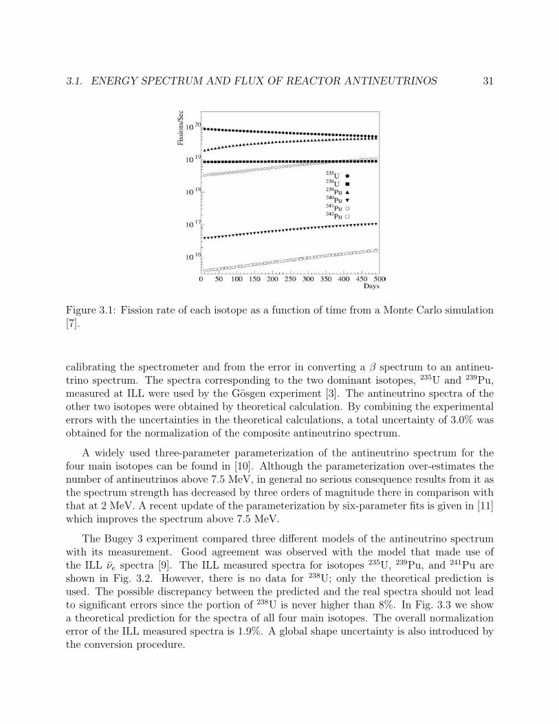
Fissile materials are continuously consumed while new fissile isotopes are bred from otherisotopes in the fuel (mainly 238U) by fast neutrons. Since the neutrino energy spectra areslightly different for the four main isotopes, the fission composition and its evolution overtime are therefore critical to the determination of the neutrino flux and energy spectrum.From the average thermal power and the effective energy released per fission [6], the averagenumber of fissions per second of each isotope can be calculated as a function of time. Fig. 3.1shows the results of computer simulation of the Palo Verde reactor cores [7].
It is common for a nuclear power plant to replace some of the fuel rods in the reactorperiodically as the fuel is used up. Typically, a reactor core will have 1/3 of its fuel changedevery 18 months. At the beginning of each refueling cycle, 69% of the fissions are from 235U,21% from 239Pu, 7% from 238U, and 3% from 241Pu. During operation the fissile isotopes239Pu and 241Pu are bred continuously from 238U. Toward the end of the fuel cycle, the fissionrates from 235U and 239Pu are about equal. The average (”standard”) fuel composition is58% of 235U, 30% of 239Pu, 7% of 238U, and 5% 241Pu [8].
The energy spectrum of the νe emitted from the fission reaction depends on the fuelcomposition. The composite antineutrino spectrum is a function of the time-dependent con-tributions of the various fissile isotopes to the fission process. The energy spectra of theantineutrinos for isotopes 235U, 239Pu, and 241Pu were deduced at ILL [9] by converting theβ spectra independently measured with a β spectrometer using 235U, 239Pu, and 241Pu tar-gets. These inferred spectra have a normalization error originating from the uncertainty in
3.1. ENERGY SPECTRUM AND FLUX OF REACTOR ANTINEUTRINOS 31
Figure 3.1: Fission rate of each isotope as a function of time from a Monte Carlo simulation[7].
calibrating the spectrometer and from the error in converting a β spectrum to an antineu-trino spectrum. The spectra corresponding to the two dominant isotopes, 235U and 239Pu,measured at ILL were used by the Gosgen experiment [3]. The antineutrino spectra of theother two isotopes were obtained by theoretical calculation. By combining the experimentalerrors with the uncertainties in the theoretical calculations, a total uncertainty of 3.0% wasobtained for the normalization of the composite antineutrino spectrum.
A widely used three-parameter parameterization of the antineutrino spectrum for thefour main isotopes can be found in [10]. Although the parameterization over-estimates thenumber of antineutrinos above 7.5 MeV, in general no serious consequence results from it asthe spectrum strength has decreased by three orders of magnitude there in comparison withthat at 2 MeV. A recent update of the parameterization by six-parameter fits is given in [11]which improves the spectrum above 7.5 MeV.
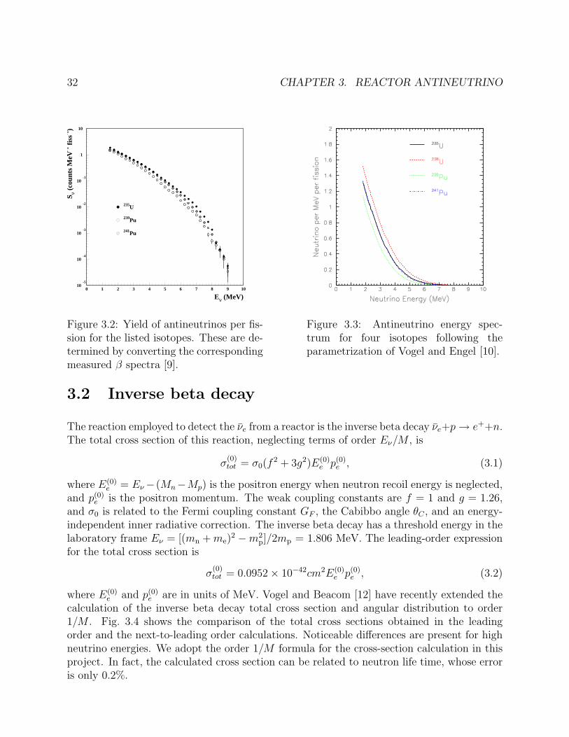
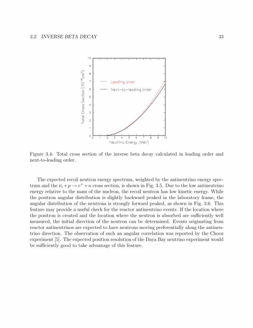
The Bugey 3 experiment compared three different models of the antineutrino spectrumwith its measurement. Good agreement was observed with the model that made use ofthe ILL νe spectra [9]. The ILL measured spectra for isotopes 235U, 239Pu, and 241Pu areshown in Fig. 3.2. However, there is no data for 238U; only the theoretical prediction isused. The possible discrepancy between the predicted and the real spectra should not leadto significant errors since the portion of 238U is never higher than 8%. In Fig. 3.3 we showa theoretical prediction for the spectra of all four main isotopes. The overall normalizationerror of the ILL measured spectra is 1.9%. A global shape uncertainty is also introduced bythe conversion procedure.
32 CHAPTER 3. REACTOR ANTINEUTRINO
10-5
10-4
10-3
10-2
10-1
1
10
0 1 2 3 4 5 6 7 8 9 10
235U
239Pu
241Pu
Eν (MeV)
S ν (c
ount
s M
eV-1
fis
s-1)
Figure 3.2: Yield of antineutrinos per fis-sion for the listed isotopes. These are de-termined by converting the correspondingmeasured β spectra [9].
Figure 3.3: Antineutrino energy spec-trum for four isotopes following theparametrization of Vogel and Engel [10].
3.2 Inverse beta decay
The reaction employed to detect the νe from a reactor is the inverse beta decay νe+p → e++n.The total cross section of this reaction, neglecting terms of order Eν/M , is
σ(0)tot = σ0(f
2 + 3g2)E(0)e p(0)
e , (3.1)
where E(0)e = Eν− (Mn−Mp) is the positron energy when neutron recoil energy is neglected,
and p(0)e is the positron momentum. The weak coupling constants are f = 1 and g = 1.26,
and σ0 is related to the Fermi coupling constant GF , the Cabibbo angle θC , and an energy-independent inner radiative correction. The inverse beta decay has a threshold energy in thelaboratory frame Eν = [(mn + me)
2 −m2p]/2mp = 1.806 MeV. The leading-order expression
for the total cross section is
σ(0)tot = 0.0952× 10−42cm2E(0)
e p(0)e , (3.2)
where E(0)e and p(0)
e are in units of MeV. Vogel and Beacom [12] have recently extended thecalculation of the inverse beta decay total cross section and angular distribution to order1/M . Fig. 3.4 shows the comparison of the total cross sections obtained in the leadingorder and the next-to-leading order calculations. Noticeable differences are present for highneutrino energies. We adopt the order 1/M formula for the cross-section calculation in thisproject. In fact, the calculated cross section can be related to neutron life time, whose erroris only 0.2%.
3.2. INVERSE BETA DECAY 33
Figure 3.4: Total cross section of the inverse beta decay calculated in leading order andnext-to-leading order.
The expected recoil neutron energy spectrum, weighted by the antineutrino energy spec-trum and the νe +p → e+ +n cross section, is shown in Fig. 3.5. Due to the low antineutrinoenergy relative to the mass of the nucleon, the recoil neutron has low kinetic energy. Whilethe positron angular distribution is slightly backward peaked in the laboratory frame, theangular distribution of the neutrons is strongly forward peaked, as shown in Fig. 3.6. Thisfeature may provide a useful check for the reactor antineutrino events. If the location wherethe positron is created and the location where the neutron is absorbed are sufficiently wellmeasured, the initial direction of the neutron can be determined. Events originating fromreactor antineutrinos are expected to have neutrons moving preferentially along the antineu-trino direction. The observation of such an angular correlation was reported by the Choozexperiment [5]. The expected position resolution of the Daya Bay neutrino experiment wouldbe sufficiently good to take advantage of this feature.
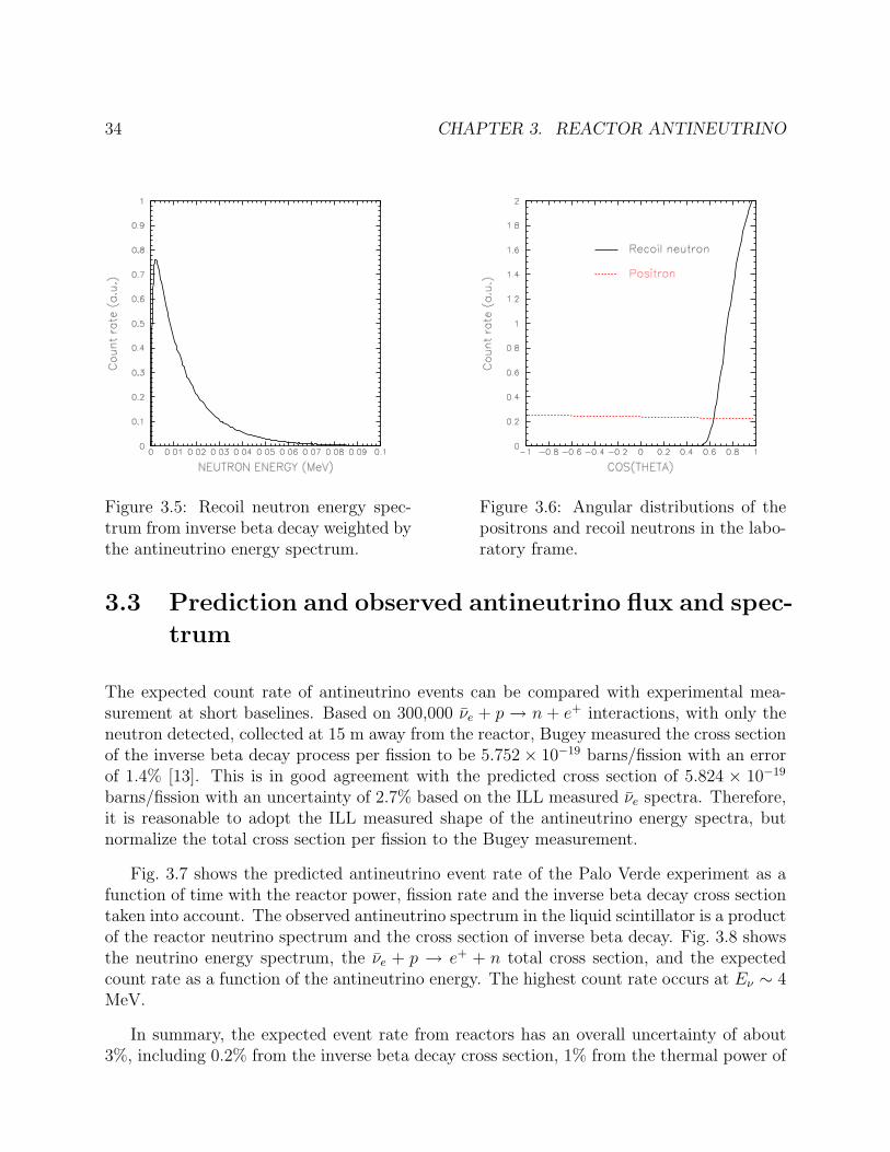
34 CHAPTER 3. REACTOR ANTINEUTRINO
Figure 3.5: Recoil neutron energy spec-trum from inverse beta decay weighted bythe antineutrino energy spectrum.
Figure 3.6: Angular distributions of thepositrons and recoil neutrons in the labo-ratory frame.
3.3 Prediction and observed antineutrino flux and spec-
trum
The expected count rate of antineutrino events can be compared with experimental mea-surement at short baselines. Based on 300,000 νe + p → n + e+ interactions, with only theneutron detected, collected at 15 m away from the reactor, Bugey measured the cross sectionof the inverse beta decay process per fission to be 5.752× 10⁻¹⁹ barns/fission with an errorof 1.4% [13]. This is in good agreement with the predicted cross section of 5.824 × 10⁻¹⁹
barns/fission with an uncertainty of 2.7% based on the ILL measured νe spectra. Therefore,it is reasonable to adopt the ILL measured shape of the antineutrino energy spectra, butnormalize the total cross section per fission to the Bugey measurement.
Fig. 3.7 shows the predicted antineutrino event rate of the Palo Verde experiment as afunction of time with the reactor power, fission rate and the inverse beta decay cross sectiontaken into account. The observed antineutrino spectrum in the liquid scintillator is a productof the reactor neutrino spectrum and the cross section of inverse beta decay. Fig. 3.8 showsthe neutrino energy spectrum, the νe + p → e+ + n total cross section, and the expectedcount rate as a function of the antineutrino energy. The highest count rate occurs at Eν ∼ 4MeV.
In summary, the expected event rate from reactors has an overall uncertainty of about3%, including 0.2% from the inverse beta decay cross section, 1% from the thermal power of
3.3. PREDICTION AND OBSERVED ANTINEUTRINO FLUX AND SPECTRUM 35
Figure 3.7: Predicted antineutrino eventrate of the Palo Verde experiment as afunction of time with the reactor power,fission rate and inverse beta decay crosssection taken into account.
Figure 3.8: Antineutrino energy spec-trum, total cross section of inverse betadecay, and count rate as a function of theantineutrino energy.
the reactors, 1% from the fuel composition and 2.5% from the energy spectra of neutrinos.
Bibliography
[1] C.L. Cowan and F. Feines, F.B. Harrison, H.W. Kruse, and A.D., McGuire, Science124, 103 (1956); Fl Reines and C.L. Cowan, Nature, 178, 446 (1956).
[2] H. Kwon et al., Phys. Rev. D24, 1097 (1981)
[3] G. Zacek et al., Phys. Rev. D34, 2621 (1986)
[4] B. Ackar et al., Nucl. Phys. B434, 503 (1995); B. Ackar et al., Phys. Lett. B374, 243(1996)
[5] M. Apollonio et al., Eur. Phys. J. C27, 331 (2003).
[6] M.F. James, J. Nucl. Energy 23 517 (1969).
[7] L. Miller, Ph.D Thesis, Stanford University, 2000, unpublished.
[8] V.I. Kopeikin, On search for new physics in nonequilibrium reactor antineutrino energyspectrum, [arXiv:hep-ph/0110030].
[9] K. Schreckenbach et al., Phys. Lett. B160, 325 (1985); A. A. Hahn et al., Phys. Lett.B218, 365 (1989).
[10] P. Vogel and J. Engel, Phys. rev. D39, 3378 (1989).
[11] P. Huber and T. Schwetz, Phys. Rev. D70, 053011 (2004) [arXiv:hep-ph/0407026].
[12] P. Vogel and J. F. Beacom, Phys. Rev. D60, 053003 (1999).
[13] Y. Declais et al., Phys. Lett. B338, 383 (1994).
36
Chapter 4
Experimental Site and LaboratoryDesigns
4.1 Overview
The Daya Bay site is an ideal place for conducting a reactor θ13 experiment. The close-by mountain range provides sufficient overburden to reduce cosmogenic background at theunderground experimental halls, making the measurement feasible. Since the Daya Baynuclear power facility consists of multiple reactors, there will be two near detectors formonitoring the yields of anti-neutrinos from these cores and one far detector to look fordisappearance of anti-neutrinos. It is possible to install another detector about half waybetween the near and far detectors to provide independent consistency checks.
The proposed experimental site is located at the east side of the Dapeng peninsula, onthe west coast of Daya Bay, where the coastline goes from southwest to northeast. It isin the Dapeng township of the Longgang Administrative District, Shenzhen Municipality,Guangdong Province. There are hills and mountain ranges on the north. The geographiclocation is east longitudinal 114◦33’00” and north latitude 22◦36’00”.
The Daya Bay Nuclear Power Plant (NPP) is situated on the southwest and the Ling AoNPP to the northeast near the coastline. Each NPP has two reactor cores that are separatedby 88 m. The distance between the centers of the two NPPs is about 1100 m. The thermalpower, Wth, of each core is 2.9 GW. Hence the total thermal power available is Wth = 11.6GW. A third NPP, called Ling Ao-II NPP, is under construction and scheduled to comeonline by 2010-2011. This NNP is built roughly along the line extended from Daya Bay toLing Ao, about 400 m northeast of Ling Ao. The core type is the same as that of the LingAo NPP but with slightly higher thermal power. When the Daya Bay-Ling Ao-Ling Ao-IINPP are all in operation, the complex can provide a total thermal power of 17.4 GW.
37
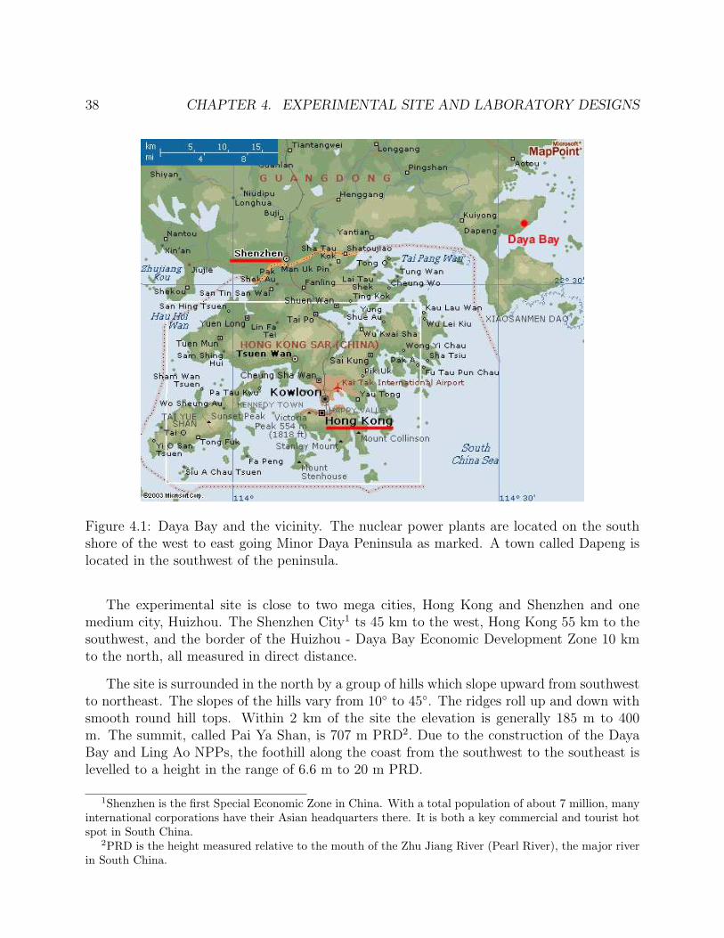
38 CHAPTER 4. EXPERIMENTAL SITE AND LABORATORY DESIGNS
Figure 4.1: Daya Bay and the vicinity. The nuclear power plants are located on the southshore of the west to east going Minor Daya Peninsula as marked. A town called Dapeng islocated in the southwest of the peninsula.
The experimental site is close to two mega cities, Hong Kong and Shenzhen and onemedium city, Huizhou. The Shenzhen City1 ts 45 km to the west, Hong Kong 55 km to thesouthwest, and the border of the Huizhou - Daya Bay Economic Development Zone 10 kmto the north, all measured in direct distance.
The site is surrounded in the north by a group of hills which slope upward from southwestto northeast. The slopes of the hills vary from 10◦ to 45◦. The ridges roll up and down withsmooth round hill tops. Within 2 km of the site the elevation is generally 185 m to 400m. The summit, called Pai Ya Shan, is 707 m PRD2. Due to the construction of the DayaBay and Ling Ao NPPs, the foothill along the coast from the southwest to the southeast islevelled to a height in the range of 6.6 m to 20 m PRD.
1Shenzhen is the first Special Economic Zone in China. With a total population of about 7 million, manyinternational corporations have their Asian headquarters there. It is both a key commercial and tourist hotspot in South China.
2PRD is the height measured relative to the mouth of the Zhu Jiang River (Pearl River), the major riverin South China.
4.2. SITE GEOLOGY 39
4.2 Site geology
Because there is yet no detailed geological survey performed specifically for the experimentalsite, the present discussion is focused on the sites of the near detectors based on the availableinformation of the Ling Ao NPP [1]. We will defer the discussion of geology of the far-detectorsite until geological survey is performed.
According to the available geological maps, the near-detector site is located in the south-west portion of the Lianhua Mountain fault, on the south side of Pai Ya Shan. It is on themassif between the Wuhua-Shenzhen and Da Pu-Haifeng sub-faults. In the vicinity of theexperimental site there are very few faults and they are not directly related to the faultsmentioned above. Hence the geological structure of the near site is rather simple.3
Surface exploration and trenching exposure show that the landforms and terrains are ingood condition. There are no karsts, landslides, collapses, mud slides, empty pockets, groundsinking asymmetry, or hot springs that would affect the stability of the site. There are onlypieces of weathered granites scattered around.
4.3 Seismic activities
According to the historical record up to December 31, 1994, there have been 63 earthquakesabove 4.7 on the Richter scale (RS), including aftershocks, within a radius of 320 km of thesite.4 Among the stronger ones, there was one 7.0 RS, one 7.3 RS, and ten 6.0 − 6.75 RS.There were 51 medium quakes between 4.7 and 5.9 RS. The strongest, 7.3 RS, took place inNan Ao in 1918. The most recent one occurred in 1969 in Yang Jiang at 6.4 RS. In addition,there have been earthquakes in the southeast foreland and one 7.3 RS quake occurred in theTaiwan Strait on Sept. 16, 1994. The epicenters of the quake were at a depth of roughly5 to 25 km. These statistics show that the seismic activities in this region originate fromshallow sources which lie in the earth crust. The strength of the quake generally decreasesfrom the shelf to inland.
Within a radius of 25 km of the experimental site, there is no record of quakes of Ms ≥3.0 (ML ≥ 3.5),5 and there is no record of even weak quakes within 5 km of the site. Thedistribution of the weak quakes is isolated in time and separated in space from one another,
3In more details, the experimental site is about 20 km from the Wuhua-Shenzhen sub-fault, and aboutthe same distance from the Da Pu-Haifeng sub-fault. It is more than 17 km from the small Daya Bay basefault. The fault scales are generally small. In particular, in the region of the planned near-detector sites,there are only four fault areas, each is no more than 300 m × 2 m.
4The seismic activities quoted here are taken from a Ling Ao NPP report [2]5Ms is the magnitude of the seismic surface wave and ML the seismic local magnitude. Ms is the normal
characteristics of an earthquake. There is a complicated location-dependent relationship between Ms andML. In Daya Bay Ms ≥ 3.0 is equivalent to ML ≥ 3.5.
40 CHAPTER 4. EXPERIMENTAL SITE AND LABORATORY DESIGNS
and without any obvious regularity.
Activity in the seismic belt of the southeast sea has shown a decreasing trend. In thenext one hundred years, this region will be in a residual energy-releasing period, followed bya calm period. It is expected that no earthquake greater than 7 RS will likely occur withina radius of 300 km around the site; the strongest seismic activity will be no more than 6RS. In conclusion, 20 years of seismic observation indicates that the region surrounding theexperimental site is in a state of low seismic activity, and there has not been any abnormalseismic activity.
4.4 Engineering geology
The following data are based on the geotechnical survey of the Ling Ao NPP. The rock ofthe near site is primarily granite, which is new or lightly effloresced. Some of the physicalproperties of the rock in this area are as follows:
• Density6: 26.3 kN/m3.
• Pressure resistance strength of a saturated single stalk: 208.4 MPa
• Pressure resistance strength of a dry single stalk: 212.1 MPa
• Softening coefficient: 0.98
• Elastic modulus: 61500 MPa
• Poisson ratio: 0.28
These properties indicate that the granite in this region is very strong and intact.
The far-detector site is about 350 m underground. It should also be sitting on lightlyeffloresced or fresh granites, sandstone or pebble rocks. The rock should have a strength andintegrity similar to that of the near site.
4.5 Hydrogeology
Daya Bay is in the semi-tropical region and the climate is dominated by the south Asiatropical monsoon. It is warm and rainy with frequent rainstorms during the typhoon seasonin one half of the year, while relatively dry in the other half. It is rare to see frost. There wasno local whether station in Daya Bay prior to mid 1982. However long term weather recordsexist in nearby Shenzhen and Hong Kong, where the yearly average temperature is 22–23◦C.
6In geology the common quoted density is the gravitational force density. In the present case it is about2.7 g/cm3 which is the density of granite.
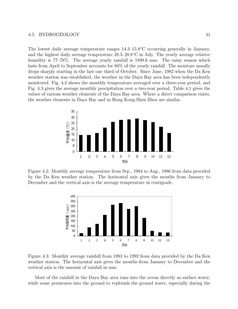
4.5. HYDROGEOLOGY 41
The lowest daily average temperature ranges 14.3–15.8◦C occurring generally in January,and the highest daily average temperature 28.3–28.8◦C in July. The yearly average relativehumidity is 77–78%. The average yearly rainfall is 1899.6 mm. The rainy season whichlasts from April to September accounts for 80% of the yearly rainfall. The moisture usuallydrops sharply starting in the last one third of October. Since June, 1982 when the Da Kenweather station was established, the weather in the Daya Bay area has been independentlymonitored. Fig. 4.2 shows the monthly temperature averaged over a three-year period, andFig. 4.3 gives the average monthly precipitation over a two-year period. Table 4.1 gives thevalues of various weather elements of the Daya Bay area. Where a direct comparison exists,the weather elements in Daya Bay and in Hong Kong-Shen Zhen are similar.
Figure 4.2: Monthly average temperature from Sep., 1984 to Aug., 1986 from data providedby the Da Ken weather station. The horizontal axis gives the months from January toDecember and the vertical axis is the average temperature in centigrade.
Figure 4.3: Monthly average rainfall from 1983 to 1992 from data provided by the Da Kenweather station. The horizontal axis gives the months from January to December and thevertical axis is the amount of rainfall in mm.
Most of the rainfall in the Daya Bay area runs into the ocean directly as surface water,while some permeates into the ground to replenish the ground water, especially during the
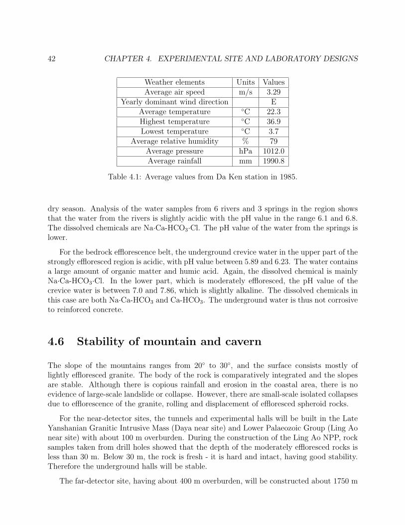
42 CHAPTER 4. EXPERIMENTAL SITE AND LABORATORY DESIGNS
Weather elements Units ValuesAverage air speed m/s 3.29
Yearly dominant wind direction EAverage temperature ◦C 22.3Highest temperature ◦C 36.9Lowest temperature ◦C 3.7
Average relative humidity % 79Average pressure hPa 1012.0Average rainfall mm 1990.8
Table 4.1: Average values from Da Ken station in 1985.
dry season. Analysis of the water samples from 6 rivers and 3 springs in the region showsthat the water from the rivers is slightly acidic with the pH value in the range 6.1 and 6.8.The dissolved chemicals are Na·Ca-HCO3·Cl. The pH value of the water from the springs islower.
For the bedrock efflorescence belt, the underground crevice water in the upper part of thestrongly effloresced region is acidic, with pH value between 5.89 and 6.23. The water containsa large amount of organic matter and humic acid. Again, the dissolved chemical is mainlyNa·Ca-HCO3·Cl. In the lower part, which is moderately effloresced, the pH value of thecrevice water is between 7.0 and 7.86, which is slightly alkaline. The dissolved chemicals inthis case are both Na·Ca-HCO3 and Ca-HCO3. The underground water is thus not corrosiveto reinforced concrete.
4.6 Stability of mountain and cavern
The slope of the mountains ranges from 20◦ to 30◦, and the surface consists mostly oflightly effloresced granite. The body of the rock is comparatively integrated and the slopesare stable. Although there is copious rainfall and erosion in the coastal area, there is noevidence of large-scale landslide or collapse. However, there are small-scale isolated collapsesdue to efflorescence of the granite, rolling and displacement of effloresced spheroid rocks.
For the near-detector sites, the tunnels and experimental halls will be built in the LateYanshanian Granitic Intrusive Mass (Daya near site) and Lower Palaeozoic Group (Ling Aonear site) with about 100 m overburden. During the construction of the Ling Ao NPP, rocksamples taken from drill holes showed that the depth of the moderately effloresced rocks isless than 30 m. Below 30 m, the rock is fresh - it is hard and intact, having good stability.Therefore the underground halls will be stable.
The far-detector site, having about 400 m overburden, will be constructed about 1750 m
4.7. TRANSPORTATION 43
north of the Daya near site. The rock along the tunnel is lightly effloresced or fresh granite.¿From a preliminary evaluation, the underground facilities again will be stable. However, itis expected that reinforcement will be needed at isolated locations where cracks may appear.
4.7 Transportation
There is no railway within a radius of 15 km of the site. The highway from Daya Bay NPPto Dapeng Township (Wang Mu) is second-class grade and 12 m wide. The Dapeng Town isconnected to Shenzhen, Hong Kong, and Guangzhou by highways which are either first-classgrade or expressways.
There are two maritime shipping lines near the site in Daya Bay, one on the east sideand the other on the west side of the Central Archipelago. Oil tankers to and from NanhaiPetrochemical use the east line. The Huizhou Harbor, which is located on the Quandaopeninsula, is 13 km north of the site. Two general-purpose 10,000-ton docks were constructedin 1989. Their functions include transporting passengers, dry goods, construction materials,and petroleum products. The ships using these two docks take the west line. The minimumdistance from the west line to the site is about 6 km. Two restricted docks of 3000-ton and5000-ton capacity, respectively, have been constructed on site during the construction of theDaya Bay NPP.
4.8 Design of laboratory facilities
The laboratory facilities include access tunnels connected to the entrance portals, a levelledmain tunnel connecting all the underground detector halls, an assembly hall, control rooms,water and electricity supplies, air ventilation, and communication. The approximate loca-tions and overburden of the near, mid, and far detector sites as well as the layout of thetunnels are shown in Fig. 4.4.
4.8.1 Detector sites
Since there are two clusters of twin reactors (will be three groups by 2010-2011) separatedin space at Daya Bay, it will need detectors close to the respective reactor cluster to monitorthe anti-neutrinos emitted from the core as precisely as possible. Detailed optimization ofthe baseline (see the chapter on Systematic for details) indicates that a near detector shouldbe positioned equidistantly from the two cores that it monitors, and should be as close tothe cores as possible. This is realized for the Daya Bay NPP. The situation for the LingAo and Ling Ao-II NPP’s is a little bit more complicated since only one near detector isused. It appears that this near detector should be equidistant from the centers of the Ling
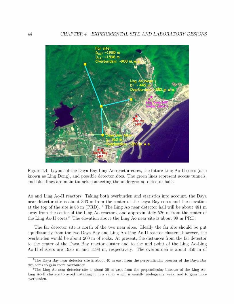
44 CHAPTER 4. EXPERIMENTAL SITE AND LABORATORY DESIGNS
Figure 4.4: Layout of the Daya Bay-Ling Ao reactor cores, the future Ling Ao-II cores (alsoknown as Ling Dong), and possible detector sites. The green lines represent access tunnels,and blue lines are main tunnels connecting the underground detector halls.
Ao and Ling Ao-II reactors. Taking both overburden and statistics into account, the Dayanear detector site is about 363 m from the center of the Daya Bay cores and the elevationat the top of the site is 88 m (PRD). 7 The Ling Ao near detector hall will be about 481 maway from the center of the Ling Ao reactors, and approximately 526 m from the center ofthe Ling Ao-II cores.8 The elevation above the Ling Ao near site is about 99 m PRD.
The far detector site is north of the two near sites. Ideally the far site should be putequidistantly from the two Daya Bay and Ling Ao-Ling Ao-II reactor clusters; however, theoverburden would be about 200 m of rocks. At present, the distances from the far detectorto the center of the Daya Bay reactor cluster and to the mid point of the Ling Ao-LingAo-II clusters are 1985 m and 1598 m, respectively. The overburden is about 350 m of
7The Daya Bay near detector site is about 40 m east from the perpendicular bisector of the Daya Baytwo cores to gain more overburden.
8The Ling Ao near detector site is about 50 m west from the perpendicular bisector of the Ling Ao-Ling Ao-II clusters to avoid installing it in a valley which is usually geologically weak, and to gain moreoverburden.
4.8. DESIGN OF LABORATORY FACILITIES 45
rocks. Precise experimental hall positions will be measured after the excavation finished,the measurement precisions from reactors to detectors could be within 5 cm. Optimizationshowed that the current location of the far detector can still meet the designed sensitivityof sin22θ13.
It is possible to install a mid detector hall between the near and far sites such that it isabout 1156 m from the Daya Bay reactor cluster and 873 m from the Ling Ao-Ling Ao-IIcluster. The elevation of mid hall is 196 m PRD. This mid experimental hall could be usedto carry out measurements for systematic studies and for internal consistency checks.
4.8.2 Tunnels
A sketch of the layout of the tunnels is shown in Fig. 4.4. There are three branches forthe horizontal main tunnel extending from a junction near the mid hall to the near andfar underground detector halls. There are also an access tunnel and a construction tunnel.The construction tunnel can be shorter if the construction tunnel goes perpendicular fromconstruction portal to the tunnel from Daya Bay near site to the junction near the mid site.
Referring to Fig. 4.4, the entrance portal of the access tunnel is behind the on-site hospitaland to the west of the Daya near site. The length of this access tunnel, from the portal tothe Daya near site, is 295 m. Its elevation is 12 m PRD, and has a grade between 8% and12% [3]. A sloped access tunnel will allow the underground facilities to go deeper, providingmore overburden. In the case of 8% grade, the elevation of the Daya near site will be -12 mPRD.
The access and main tunnels will be able to accommodate vehicles transporting equip-ment of different size and weight. A conceptual design of the tunnel is shown in Fig. 4.5. Ithas an inverse-U shape. The height, as well as the width, is 7.2 m. The grade of the maintunnel will be at most 0.3% to ensure levelled movement of the heavy detectors filled withliquid scintillator inside the main tunnel. The lowest position will be near the Daya Baynear site where a pool will be built to collect the leak water in the tunnel. From there thewater will be pumped out to the outside of the tunnel.
The entrance portal of the construction tunnel is at the upper level of the Daya BayQuarry (see Fig. 4.4). The length of this tunnel is 607 m from the entrance to the junctionnear the mid site [3]. During excavation, all the waste rocks and dirt are transferred throughthis tunnel to the outside. This construction tunnel is also necessary to avoid the interferenceof excavation activities from the assembly of detectors in the Daya near and mid sites. Thecross section of the construction tunnel can be smaller than the access and main tunnel butit is large enough for tramcar transportation. The grade can be as large as 33%.
The total length of the tunnel is 3094 m. The amount of waste to be removed will be120000 m3 (this is a scaled number) [3]. About half of the waste will be stacked up in theDaya Bay Quarry to provide additional overburden to the Daya near site which is not far
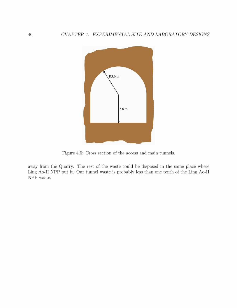
46 CHAPTER 4. EXPERIMENTAL SITE AND LABORATORY DESIGNS
Figure 4.5: Cross section of the access and main tunnels.
away from the Quarry. The rest of the waste could be disposed in the same place whereLing Ao-II NPP put it. Our tunnel waste is probably less than one tenth of the Ling Ao-IINPP waste.
Bibliography
[1] Report of Ling Ao Nuclear Power Plant.
[2] Catalog of Chinese Earthquakes, Quoted in the Preliminary Safety Report on Ling AoNuclear Power Plant.
[3] Report of Preliminary Feasibility Study of Site Selection for the Daya Bay NeutrinoExperiment, prepared by Beijing Institute of Nuclear Energy, September, 2004.
47

48 BIBLIOGRAPHY
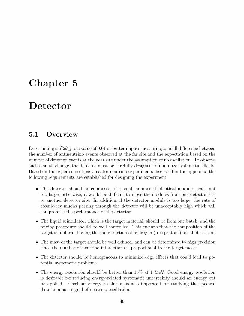
Chapter 5
Detector
5.1 Overview
Determining sin22θ13 to a value of 0.01 or better implies measuring a small difference betweenthe number of antineutrino events observed at the far site and the expectation based on thenumber of detected events at the near site under the assumption of no oscillation. To observesuch a small change, the detector must be carefully designed to minimize systematic effects.Based on the experience of past reactor neutrino experiments discussed in the appendix, thefollowing requirements are established for designing the experiment:
• The detector should be composed of a small number of identical modules, each nottoo large; otherwise, it would be difficult to move the modules from one detector siteto another detector site. In addition, if the detector module is too large, the rate ofcosmic-ray muons passing through the detector will be unacceptably high which willcompromise the performance of the detector.
• The liquid scintillator, which is the target material, should be from one batch, and themixing procedure should be well controlled. This ensures that the composition of thetarget is uniform, having the same fraction of hydrogen (free protons) for all detectors.
• The mass of the target should be well defined, and can be determined to high precisionsince the number of neutrino interactions is proportional to the target mass.
• The detector should be homogeneous to minimize edge effects that could lead to po-tential systematic problems.
• The energy resolution should be better than 15% at 1 MeV. Good energy resolutionis desirable for reducing energy-related systematic uncertainty should an energy cutbe applied. Excellent energy resolution is also important for studying the spectraldistortion as a signal of neutrino oscillation.
49
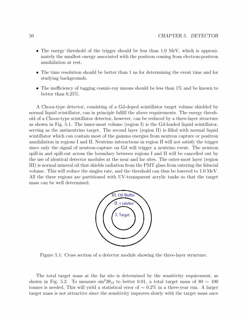
50 CHAPTER 5. DETECTOR
• The energy threshold of the trigger should be less than 1.0 MeV, which is approxi-mately the smallest energy associated with the positron coming from electron-positronannihilation at rest.
• The time resolution should be better than 1 ns for determining the event time and forstudying backgrounds.
• The inefficiency of tagging cosmic-ray muons should be less than 1% and be known tobetter than 0.25%.
A Chooz-type detector, consisting of a Gd-doped scintillator target volume shielded bynormal liquid scintillator, can in principle fulfill the above requirements. The energy thresh-old of a Chooz-type scintillator detector, however, can be reduced by a three-layer structureas shown in Fig. 5.1. The inner-most volume (region I) is the Gd-loaded liquid scintillator,serving as the antineutrino target. The second layer (region II) is filled with normal liquidscintillator which can contain most of the gamma energies from neutron capture or positronannihilation in regions I and II. Neutrino interactions in region II will not satisfy the triggersince only the signal of neutron-capture on Gd will trigger a neutrino event. The neutronspill-in and spill-out across the boundary between regions I and II will be cancelled out bythe use of identical detector modules at the near and far sites. The outer-most layer (regionIII) is normal mineral oil that shields radiation from the PMT glass from entering the fiducialvolume. This will reduce the singles rate, and the threshold can thus be lowered to 1.0 MeV.All the three regions are partitioned with UV-transparent acrylic tanks so that the targetmass can be well determined.
Figure 5.1: Cross section of a detector module showing the three-layer structure.
The total target mass at the far site is determined by the sensitivity requirement, asshown in Fig. 5.2. To measure sin22θ13 to better 0.01, a total target mass of 80 ∼ 100tonnes is needed, This will yield a statistical error of ∼ 0.2% in a three-year run. A largertarget mass is not attractive since the sensitivity improves slowly with the target mass once
5.1. OVERVIEW 51
the measurement is systematic-limited. In order to have sufficient target mass at the farsite, a scheme with multiple detector modules, each with a typical target mass of 20 metrictons, is chosen. Identical detector modules, fewer in number, will be used at the near sites.The scheme of multiple modules offers better scalability and internal consistency checks at agiven location. The 20-ton modules are easier to construct, less susceptible to cosmic-muoninduced backgrounds, and easier to move. Movable detector modules will allow us to swapdetectors between the far and near sites, further reducing detector systematic errors. Inaddition, adjusting the baseline is possible for movable detectors.
0
0.005
0.01
0.015
0.02
0.025
0.03
0 50 100 150 200
∆m2 = 2.0×10⁻³eV2
σsys = 0.2%
(B/S)Near = 0.5%
(B/S)Mid = 0.1%
(B/S)Far = 0.1%
Target Mass at Far Site (Ton)
sin2 2θ
13 S
ensi
tivi
ty
Figure 5.2: Sensitivity of sin22θ13 at 90% C.L. as a function of target mass at the far site.
Each detector module will be viewed by about 200 8” PMTs with low-radioactivity glass.1
At the near site (360-500 m from reactors), about 400 to 800 νe events per day per modulecan be obtained at the Daya Bay nuclear power complex, while about 70 events per day permodule can be obtained at the far site (∼ 1700m).2 For the near detector, two modules arenecessary in order to have cross checks. For the far detector, four modules are needed inorder to have enough statistics to reach the designed sensitivity while keeping the numberof modules at a manageable level. To minimize the differences in systematic uncertaintiesbetween the near and far locations, detector modules can be cross calibrated at the near site
1The detector of Chooz had a mass of 5 tonnes, Palo Verde 12 tonnes with fine segmentation, MiniBooNE800 tonnes, and KamLAND 1000 tonnes,
2At a distance of 1 km, the rate is about 1 νe event per GW per tonne per day.
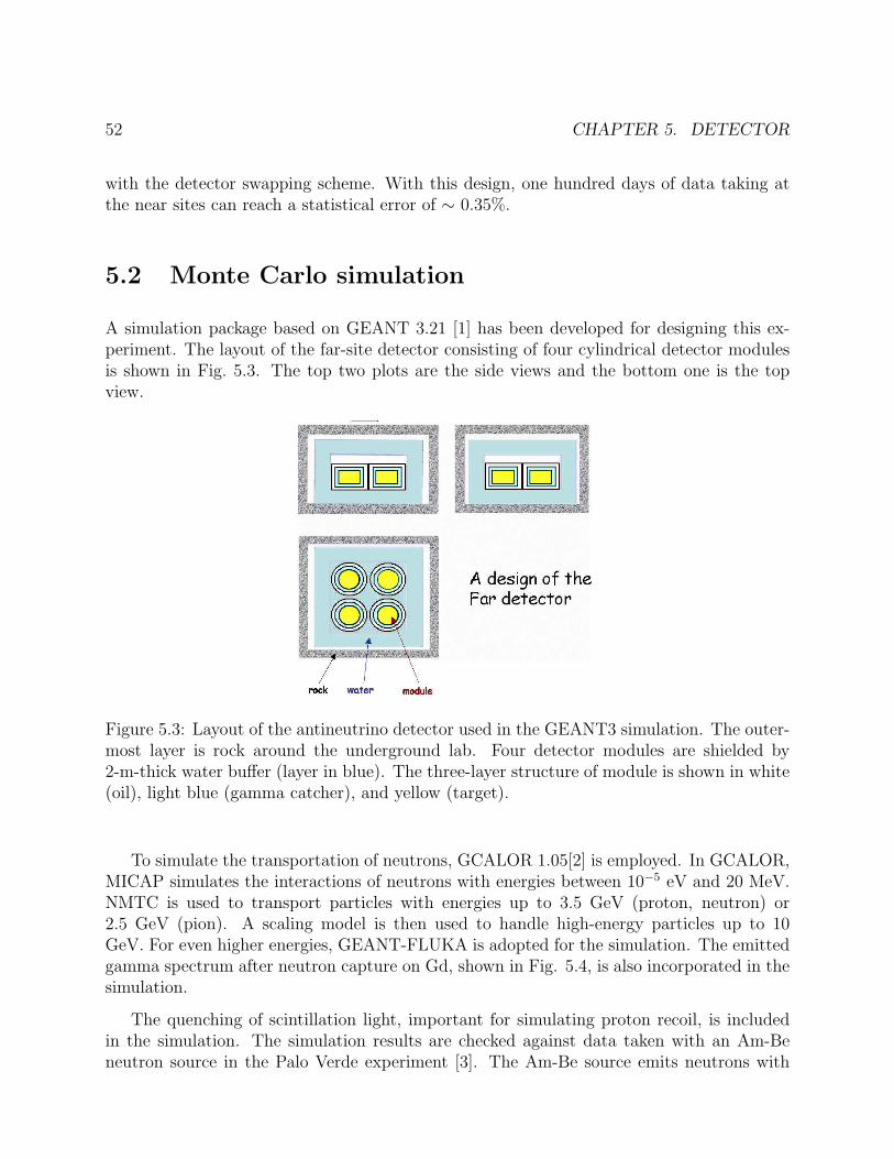
52 CHAPTER 5. DETECTOR
with the detector swapping scheme. With this design, one hundred days of data taking atthe near sites can reach a statistical error of ∼ 0.35%.
5.2 Monte Carlo simulation
A simulation package based on GEANT 3.21 [1] has been developed for designing this ex-periment. The layout of the far-site detector consisting of four cylindrical detector modulesis shown in Fig. 5.3. The top two plots are the side views and the bottom one is the topview.
Figure 5.3: Layout of the antineutrino detector used in the GEANT3 simulation. The outer-most layer is rock around the underground lab. Four detector modules are shielded by2-m-thick water buffer (layer in blue). The three-layer structure of module is shown in white(oil), light blue (gamma catcher), and yellow (target).
To simulate the transportation of neutrons, GCALOR 1.05[2] is employed. In GCALOR,MICAP simulates the interactions of neutrons with energies between 10−5 eV and 20 MeV.NMTC is used to transport particles with energies up to 3.5 GeV (proton, neutron) or2.5 GeV (pion). A scaling model is then used to handle high-energy particles up to 10GeV. For even higher energies, GEANT-FLUKA is adopted for the simulation. The emittedgamma spectrum after neutron capture on Gd, shown in Fig. 5.4, is also incorporated in thesimulation.
The quenching of scintillation light, important for simulating proton recoil, is includedin the simulation. The simulation results are checked against data taken with an Am-Beneutron source in the Palo Verde experiment [3]. The Am-Be source emits neutrons with
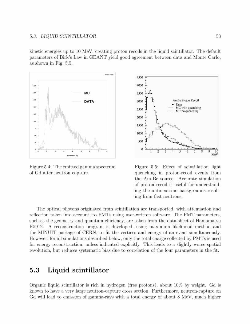
5.3. LIQUID SCINTILLATOR 53
kinetic energies up to 10 MeV, creating proton recoils in the liquid scintillator. The defaultparameters of Birk’s Law in GEANT yield good agreement between data and Monte Carlo,as shown in Fig. 5.5.
generated Eg
96/09/25 09.55
MC
DATA
0
25
50
75
100
125
150
175
200
225
0 1 2 3 4 5 6 7 8
Figure 5.4: The emitted gamma spectrumof Gd after neutron capture.
Figure 5.5: Effect of scintillation lightquenching in proton-recoil events fromthe Am-Be source. Accurate simulationof proton recoil is useful for understand-ing the antineutrino backgrounds result-ing from fast neutrons.
The optical photons originated from scintillation are transported, with attenuation andreflection taken into account, to PMTs using user-written software. The PMT parameters,such as the geometry and quantum efficiency, are taken from the data sheet of HamamatsuR5912. A reconstruction program is developed, using maximum likelihood method andthe MINUIT package of CERN, to fit the vertices and energy of an event simultaneously.However, for all simulations described below, only the total charge collected by PMTs is usedfor energy reconstruction, unless indicated explicitly. This leads to a slightly worse spatialresolution, but reduces systematic bias due to correlation of the four parameters in the fit.
5.3 Liquid scintillator
Organic liquid scintillator is rich in hydrogen (free protons), about 10% by weight. Gd isknown to have a very large neutron-capture cross section. Furthermore, neutron-capture onGd will lead to emission of gamma-rays with a total energy of about 8 MeV, much higher
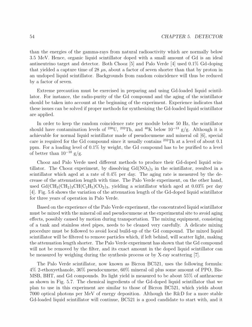
54 CHAPTER 5. DETECTOR
than the energies of the gamma-rays from natural radioactivity which are normally below3.5 MeV. Hence, organic liquid scintillator doped with a small amount of Gd is an idealantineutrino target and detector. Both Chooz [5] and Palo Verde [4] used 0.1% Gd-dopingthat yielded a capture time of 28 µs, about a factor of seven shorter than that by proton inan undoped liquid scintillator. Backgrounds from random coincidence will thus be reducedby a factor of seven.
Extreme precaution must be exercised in preparing and using Gd-loaded liquid scintil-lator. For instance, the radio-purity of the Gd compound and the aging of the scintillatorshould be taken into account at the beginning of the experiment. Experience indicates thatthese issues can be solved if proper methods for synthesizing the Gd-loaded liquid scintillatorare applied.
In order to keep the random coincidence rate per module below 50 Hz, the scintillatorshould have contamination levels of 238U, 232Th, and 40K below 10−13 g/g. Although it isachievable for normal liquid scintillator made of pseudocumene and mineral oil [6], specialcare is required for the Gd compound since it usually contains 232Th at a level of about 0.1ppm. For a loading level of 0.1% by weight, the Gd compound has to be purified to a levelof better than 10−10 g/g.
Chooz and Palo Verde used different methods to produce their Gd-doped liquid scin-tillator. The Chooz experiment, by dissolving Gd(NO3)3 in the scintillator, resulted in ascintillator which aged at a rate of 0.4% per day. The aging rate is measured by the de-crease of the attenuation length with time. The Palo Verde experiment, on the other hand,used Gd(CH3(CH2)3CH(C2H5)CO2)3, yielding a scintillator which aged at 0.03% per day[4]. Fig. 5.6 shows the variation of the attenuation length of the Gd-doped liquid scintillatorfor three years of operation in Palo Verde.
Based on the experience of the Palo Verde experiment, the concentrated liquid scintillatormust be mixed with the mineral oil and pseudocumene at the experimental site to avoid agingeffects, possibly caused by motion during transportation. The mixing equipment, consistingof a tank and stainless steel pipes, needs to be cleaned very carefully. A delicate mixingprocedure must be followed to avoid local build-up of the Gd compound. The mixed liquidscintillator will be filtered to remove particles which, if left behind, will scatter light, makingthe attenuation length shorter. The Palo Verde experiment has shown that the Gd compoundwill not be removed by the filter, and its exact amount in the doped liquid scintillator canbe measured by weighing during the synthesis process or by X-ray scattering [7].
The Palo Verde scintillator, now known as Bicron BC521, uses the following formula:4% 2-ethoxyethanole, 36% pseudocumene, 60% mineral oil plus some amount of PPO, Bis-MSB, BHT, and Gd compounds. Its light yield is measured to be about 55% of anthraceneas shown in Fig. 5.7. The chemical ingredients of the Gd-doped liquid scintillator that weplan to use in this experiment are similar to those of Bicron BC521, which yields about7000 optical photons per MeV of energy deposition. Although the R&D for a more stableGd-loaded liquid scintillator will continue, BC521 is a good candidate to start with, and it
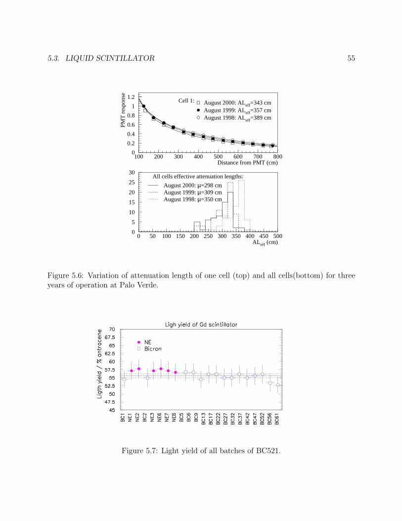
5.3. LIQUID SCINTILLATOR 55
Cell 1: August 2000: ALeff=343 cmAugust 1999: ALeff=357 cmAugust 1998: ALeff=389 cm
Distance from PMT (cm)
PMT
res
pons
e
ALeff (cm)
All cells effective attenuation lengths:
August 2000: µ=298 cmAugust 1999: µ=309 cmAugust 1998: µ=350 cm
0
0.2
0.4
0.6
0.8
1
1.2
100 200 300 400 500 600 700 800
0
5
10
15
20
25
30
0 50 100 150 200 250 300 350 400 450 500
Figure 5.6: Variation of attenuation length of one cell (top) and all cells(bottom) for threeyears of operation at Palo Verde.
Figure 5.7: Light yield of all batches of BC521.

56 CHAPTER 5. DETECTOR
fulfills our requirements.
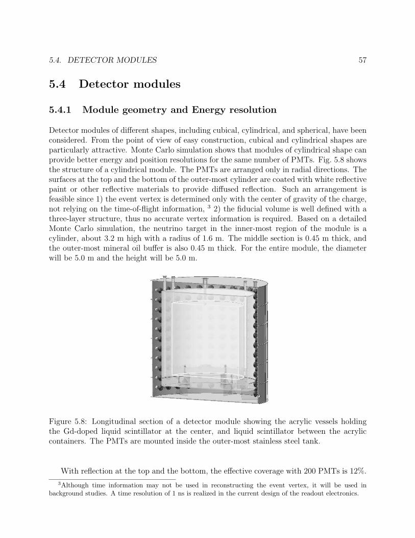
5.4. DETECTOR MODULES 57
5.4 Detector modules
5.4.1 Module geometry and Energy resolution
Detector modules of different shapes, including cubical, cylindrical, and spherical, have beenconsidered. From the point of view of easy construction, cubical and cylindrical shapes areparticularly attractive. Monte Carlo simulation shows that modules of cylindrical shape canprovide better energy and position resolutions for the same number of PMTs. Fig. 5.8 showsthe structure of a cylindrical module. The PMTs are arranged only in radial directions. Thesurfaces at the top and the bottom of the outer-most cylinder are coated with white reflectivepaint or other reflective materials to provide diffused reflection. Such an arrangement isfeasible since 1) the event vertex is determined only with the center of gravity of the charge,not relying on the time-of-flight information, 3 2) the fiducial volume is well defined with athree-layer structure, thus no accurate vertex information is required. Based on a detailedMonte Carlo simulation, the neutrino target in the inner-most region of the module is acylinder, about 3.2 m high with a radius of 1.6 m. The middle section is 0.45 m thick, andthe outer-most mineral oil buffer is also 0.45 m thick. For the entire module, the diameterwill be 5.0 m and the height will be 5.0 m.
Figure 5.8: Longitudinal section of a detector module showing the acrylic vessels holdingthe Gd-doped liquid scintillator at the center, and liquid scintillator between the acryliccontainers. The PMTs are mounted inside the outer-most stainless steel tank.
With reflection at the top and the bottom, the effective coverage with 200 PMTs is 12%.
3Although time information may not be used in reconstructing the event vertex, it will be used inbackground studies. A time resolution of 1 ns is realized in the current design of the readout electronics.
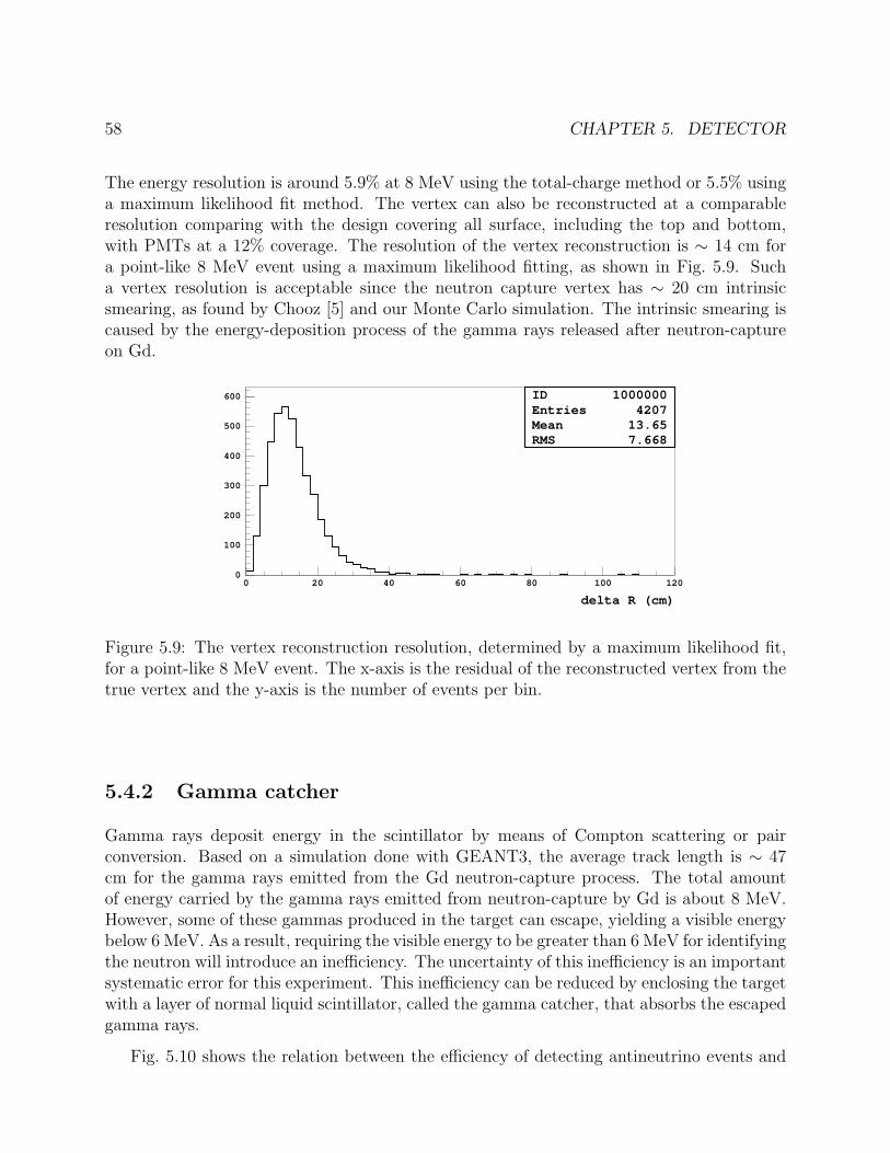
58 CHAPTER 5. DETECTOR
The energy resolution is around 5.9% at 8 MeV using the total-charge method or 5.5% usinga maximum likelihood fit method. The vertex can also be reconstructed at a comparableresolution comparing with the design covering all surface, including the top and bottom,with PMTs at a 12% coverage. The resolution of the vertex reconstruction is ∼ 14 cm fora point-like 8 MeV event using a maximum likelihood fitting, as shown in Fig. 5.9. Sucha vertex resolution is acceptable since the neutron capture vertex has ∼ 20 cm intrinsicsmearing, as found by Chooz [5] and our Monte Carlo simulation. The intrinsic smearing iscaused by the energy-deposition process of the gamma rays released after neutron-captureon Gd.
IDEntriesMeanRMS
1000000 4207
13.65 7.668
delta R (cm)
0
100
200
300
400
500
600
0 20 40 60 80 100 120
Figure 5.9: The vertex reconstruction resolution, determined by a maximum likelihood fit,for a point-like 8 MeV event. The x-axis is the residual of the reconstructed vertex from thetrue vertex and the y-axis is the number of events per bin.
5.4.2 Gamma catcher
Gamma rays deposit energy in the scintillator by means of Compton scattering or pairconversion. Based on a simulation done with GEANT3, the average track length is ∼ 47cm for the gamma rays emitted from the Gd neutron-capture process. The total amountof energy carried by the gamma rays emitted from neutron-capture by Gd is about 8 MeV.However, some of these gammas produced in the target can escape, yielding a visible energybelow 6 MeV. As a result, requiring the visible energy to be greater than 6 MeV for identifyingthe neutron will introduce an inefficiency. The uncertainty of this inefficiency is an importantsystematic error for this experiment. This inefficiency can be reduced by enclosing the targetwith a layer of normal liquid scintillator, called the gamma catcher, that absorbs the escapedgamma rays.
Fig. 5.10 shows the relation between the efficiency of detecting antineutrino events and
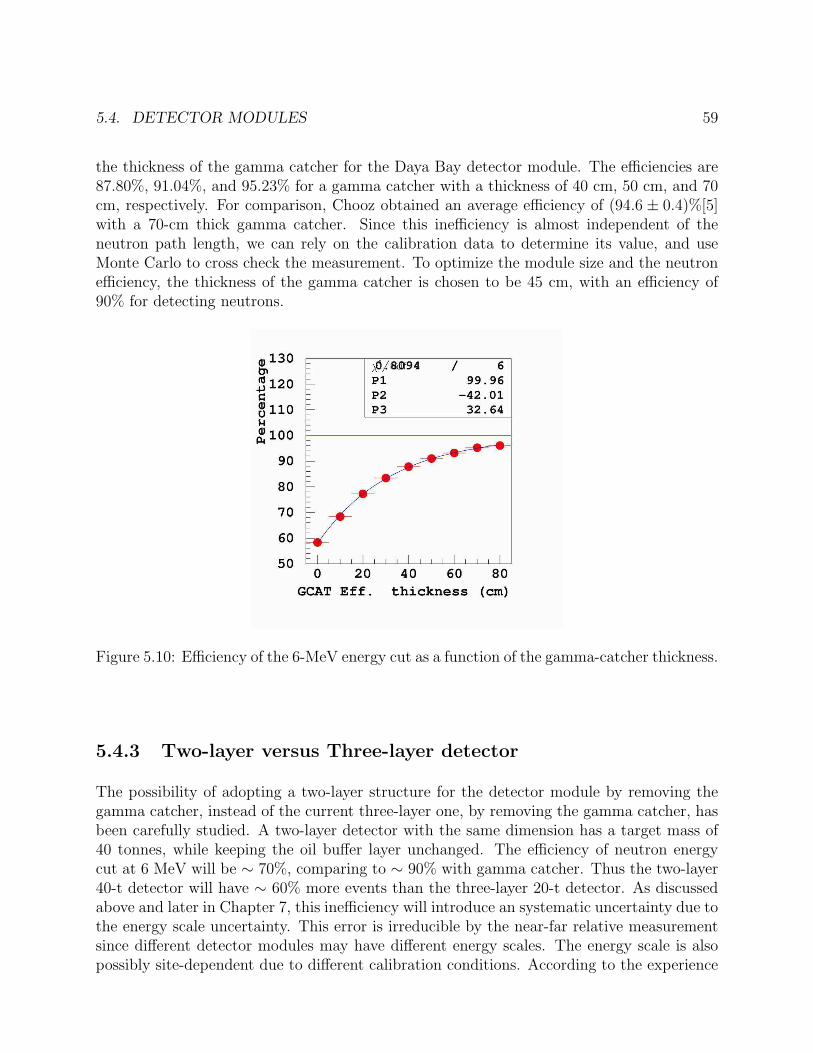
5.4. DETECTOR MODULES 59
the thickness of the gamma catcher for the Daya Bay detector module. The efficiencies are87.80%, 91.04%, and 95.23% for a gamma catcher with a thickness of 40 cm, 50 cm, and 70cm, respectively. For comparison, Chooz obtained an average efficiency of (94.6 ± 0.4)%[5]with a 70-cm thick gamma catcher. Since this inefficiency is almost independent of theneutron path length, we can rely on the calibration data to determine its value, and useMonte Carlo to cross check the measurement. To optimize the module size and the neutronefficiency, the thickness of the gamma catcher is chosen to be 45 cm, with an efficiency of90% for detecting neutrons.
Figure 5.10: Efficiency of the 6-MeV energy cut as a function of the gamma-catcher thickness.
5.4.3 Two-layer versus Three-layer detector
The possibility of adopting a two-layer structure for the detector module by removing thegamma catcher, instead of the current three-layer one, by removing the gamma catcher, hasbeen carefully studied. A two-layer detector with the same dimension has a target mass of40 tonnes, while keeping the oil buffer layer unchanged. The efficiency of neutron energycut at 6 MeV will be ∼ 70%, comparing to ∼ 90% with gamma catcher. Thus the two-layer40-t detector will have ∼ 60% more events than the three-layer 20-t detector. As discussedabove and later in Chapter 7, this inefficiency will introduce an systematic uncertainty due tothe energy scale uncertainty. This error is irreducible by the near-far relative measurementsince different detector modules may have different energy scales. The energy scale is alsopossibly site-dependent due to different calibration conditions. According to the experience
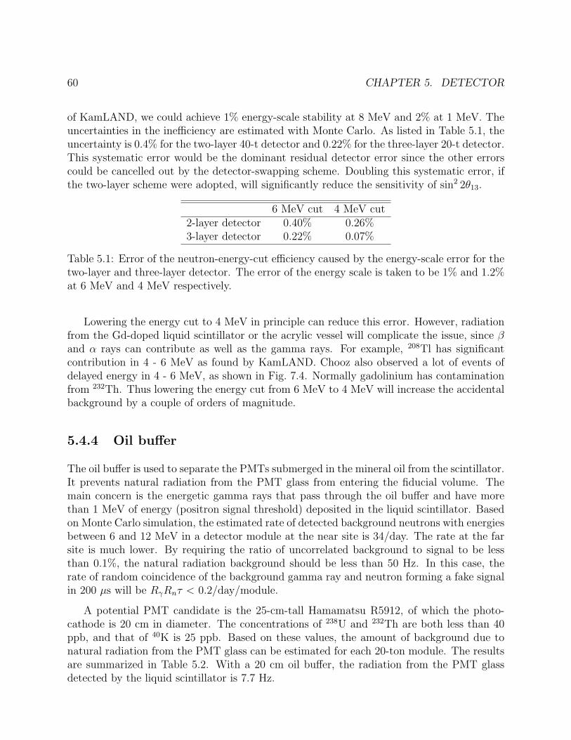
60 CHAPTER 5. DETECTOR
of KamLAND, we could achieve 1% energy-scale stability at 8 MeV and 2% at 1 MeV. Theuncertainties in the inefficiency are estimated with Monte Carlo. As listed in Table 5.1, theuncertainty is 0.4% for the two-layer 40-t detector and 0.22% for the three-layer 20-t detector.This systematic error would be the dominant residual detector error since the other errorscould be cancelled out by the detector-swapping scheme. Doubling this systematic error, ifthe two-layer scheme were adopted, will significantly reduce the sensitivity of sin2 2θ13.
6 MeV cut 4 MeV cut2-layer detector 0.40% 0.26%3-layer detector 0.22% 0.07%
Table 5.1: Error of the neutron-energy-cut efficiency caused by the energy-scale error for thetwo-layer and three-layer detector. The error of the energy scale is taken to be 1% and 1.2%at 6 MeV and 4 MeV respectively.
Lowering the energy cut to 4 MeV in principle can reduce this error. However, radiationfrom the Gd-doped liquid scintillator or the acrylic vessel will complicate the issue, since βand α rays can contribute as well as the gamma rays. For example, 208Tl has significantcontribution in 4 - 6 MeV as found by KamLAND. Chooz also observed a lot of events ofdelayed energy in 4 - 6 MeV, as shown in Fig. 7.4. Normally gadolinium has contaminationfrom 232Th. Thus lowering the energy cut from 6 MeV to 4 MeV will increase the accidentalbackground by a couple of orders of magnitude.
5.4.4 Oil buffer
The oil buffer is used to separate the PMTs submerged in the mineral oil from the scintillator.It prevents natural radiation from the PMT glass from entering the fiducial volume. Themain concern is the energetic gamma rays that pass through the oil buffer and have morethan 1 MeV of energy (positron signal threshold) deposited in the liquid scintillator. Basedon Monte Carlo simulation, the estimated rate of detected background neutrons with energiesbetween 6 and 12 MeV in a detector module at the near site is 34/day. The rate at the farsite is much lower. By requiring the ratio of uncorrelated background to signal to be lessthan 0.1%, the natural radiation background should be less than 50 Hz. In this case, therate of random coincidence of the background gamma ray and neutron forming a fake signalin 200 µs will be RγRnτ < 0.2/day/module.
A potential PMT candidate is the 25-cm-tall Hamamatsu R5912, of which the photo-cathode is 20 cm in diameter. The concentrations of 238U and 232Th are both less than 40ppb, and that of 40K is 25 ppb. Based on these values, the amount of background due tonatural radiation from the PMT glass can be estimated for each 20-ton module. The resultsare summarized in Table 5.2. With a 20 cm oil buffer, the radiation from the PMT glassdetected by the liquid scintillator is 7.7 Hz.
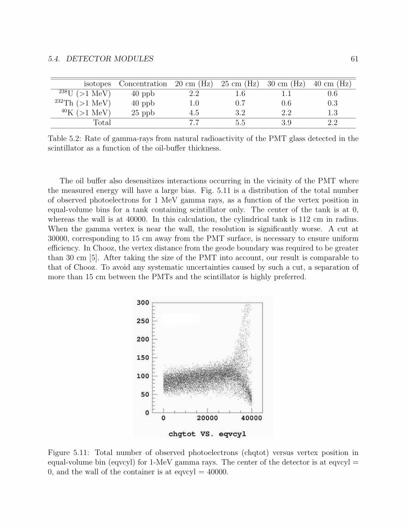
5.4. DETECTOR MODULES 61
isotopes Concentration 20 cm (Hz) 25 cm (Hz) 30 cm (Hz) 40 cm (Hz)238U (>1 MeV) 40 ppb 2.2 1.6 1.1 0.6
232Th (>1 MeV) 40 ppb 1.0 0.7 0.6 0.340K (>1 MeV) 25 ppb 4.5 3.2 2.2 1.3
Total 7.7 5.5 3.9 2.2
Table 5.2: Rate of gamma-rays from natural radioactivity of the PMT glass detected in thescintillator as a function of the oil-buffer thickness.
The oil buffer also desensitizes interactions occurring in the vicinity of the PMT wherethe measured energy will have a large bias. Fig. 5.11 is a distribution of the total numberof observed photoelectrons for 1 MeV gamma rays, as a function of the vertex position inequal-volume bins for a tank containing scintillator only. The center of the tank is at 0,whereas the wall is at 40000. In this calculation, the cylindrical tank is 112 cm in radius.When the gamma vertex is near the wall, the resolution is significantly worse. A cut at30000, corresponding to 15 cm away from the PMT surface, is necessary to ensure uniformefficiency. In Chooz, the vertex distance from the geode boundary was required to be greaterthan 30 cm [5]. After taking the size of the PMT into account, our result is comparable tothat of Chooz. To avoid any systematic uncertainties caused by such a cut, a separation ofmore than 15 cm between the PMTs and the scintillator is highly preferred.
Figure 5.11: Total number of observed photoelectrons (chqtot) versus vertex position inequal-volume bin (eqvcyl) for 1-MeV gamma rays. The center of the detector is at eqvcyl =0, and the wall of the container is at eqvcyl = 40000.
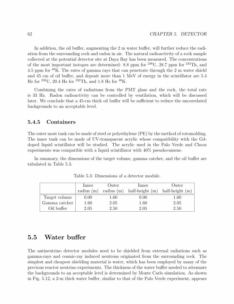
62 CHAPTER 5. DETECTOR
In addition, the oil buffer, augmenting the 2 m water buffer, will further reduce the radi-ation from the surrounding rock and radon in air. The natural radioactivity of a rock samplecollected at the potential detector site at Daya Bay has been measured. The concentrationsof the most important isotopes are determined: 8.8 ppm for 238U, 28.7 ppm for 232Th, and4.5 ppm for 40K. The rates of gamma rays that can penetrate through the 2 m water shieldand 45 cm of oil buffer, and deposit more than 1 MeV of energy in the scintillator are 5.4Hz for 238U, 20.4 Hz for 232Th, and 1.8 Hz for 40K.
Combining the rates of radiations from the PMT glass and the rock, the total rateis 33 Hz. Radon radioactivity can be controlled by ventilation, which will be discussedlater. We conclude that a 45-cm thick oil buffer will be sufficient to reduce the uncorrelatedbackgrounds to an acceptable level.
5.4.5 Containers
The outer most tank can be made of steel or polyethylene (PE) by the method of rotomolding.The inner tank can be made of UV-transparent acrylic whose compatibility with the Gd-doped liquid scintillator will be studied. The acrylic used in the Palo Verde and Choozexperiments was compatible with a liquid scintillator with 40% pseudocumene.
In summary, the dimensions of the target volume, gamma catcher, and the oil buffer aretabulated in Table 5.3.
Table 5.3: Dimensions of a detector module.
Inner Outer Inner Outerradius (m) radius (m) half-height (m) half-height (m)
Target volume 0.00 1.60 0.00 1.60Gamma catcher 1.60 2.05 1.60 2.05
Oil buffer 2.05 2.50 2.05 2.50
5.5 Water buffer
The antineutrino detector modules need to be shielded from external radiations such asgamma-rays and cosmic-ray induced neutrons originated from the surrounding rock. Thesimplest and cheapest shielding material is water, which has been employed by many of theprevious reactor neutrino experiments. The thickness of the water buffer needed to attenuatethe backgrounds to an acceptable level is determined by Monte Carlo simulation. As shownin Fig. 5.12, a 2-m thick water buffer, similar to that of the Palo Verde experiment, appears
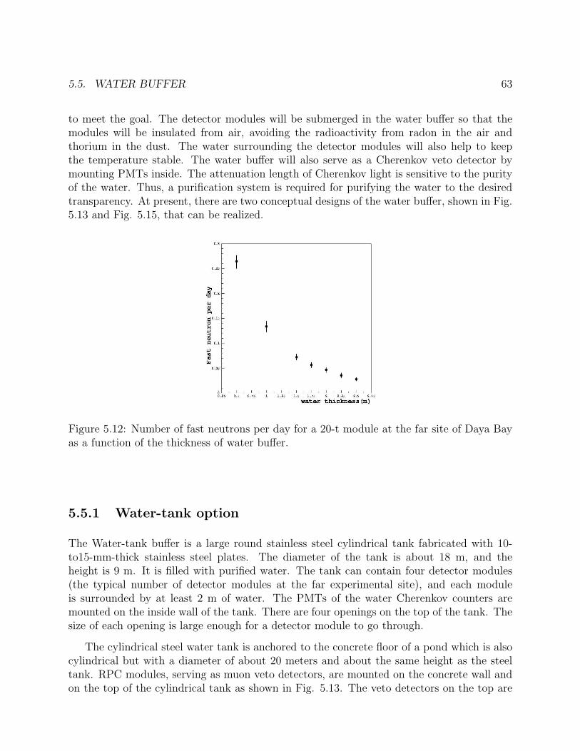
5.5. WATER BUFFER 63
to meet the goal. The detector modules will be submerged in the water buffer so that themodules will be insulated from air, avoiding the radioactivity from radon in the air andthorium in the dust. The water surrounding the detector modules will also help to keepthe temperature stable. The water buffer will also serve as a Cherenkov veto detector bymounting PMTs inside. The attenuation length of Cherenkov light is sensitive to the purityof the water. Thus, a purification system is required for purifying the water to the desiredtransparency. At present, there are two conceptual designs of the water buffer, shown in Fig.5.13 and Fig. 5.15, that can be realized.
Figure 5.12: Number of fast neutrons per day for a 20-t module at the far site of Daya Bayas a function of the thickness of water buffer.
5.5.1 Water-tank option
The Water-tank buffer is a large round stainless steel cylindrical tank fabricated with 10-to15-mm-thick stainless steel plates. The diameter of the tank is about 18 m, and theheight is 9 m. It is filled with purified water. The tank can contain four detector modules(the typical number of detector modules at the far experimental site), and each moduleis surrounded by at least 2 m of water. The PMTs of the water Cherenkov counters aremounted on the inside wall of the tank. There are four openings on the top of the tank. Thesize of each opening is large enough for a detector module to go through.
The cylindrical steel water tank is anchored to the concrete floor of a pond which is alsocylindrical but with a diameter of about 20 meters and about the same height as the steeltank. RPC modules, serving as muon veto detectors, are mounted on the concrete wall andon the top of the cylindrical tank as shown in Fig. 5.13. The veto detectors on the top are
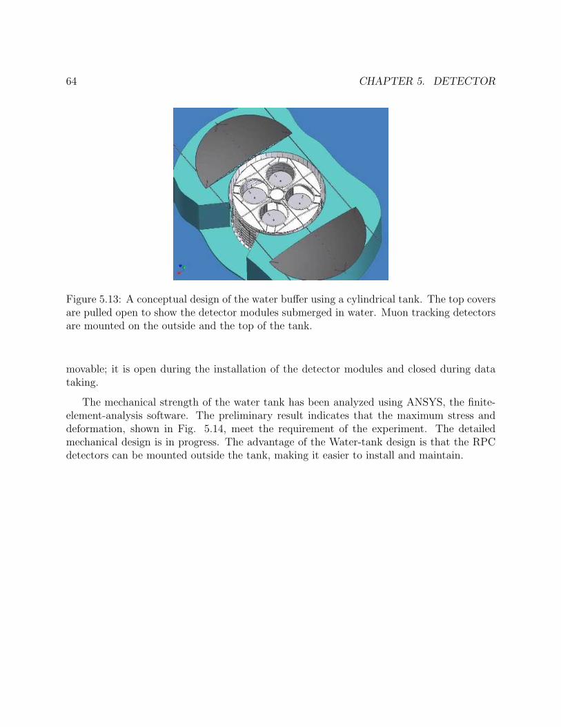
64 CHAPTER 5. DETECTOR
Figure 5.13: A conceptual design of the water buffer using a cylindrical tank. The top coversare pulled open to show the detector modules submerged in water. Muon tracking detectorsare mounted on the outside and the top of the tank.
movable; it is open during the installation of the detector modules and closed during datataking.
The mechanical strength of the water tank has been analyzed using ANSYS, the finite-element-analysis software. The preliminary result indicates that the maximum stress anddeformation, shown in Fig. 5.14, meet the requirement of the experiment. The detailedmechanical design is in progress. The advantage of the Water-tank design is that the RPCdetectors can be mounted outside the tank, making it easier to install and maintain.
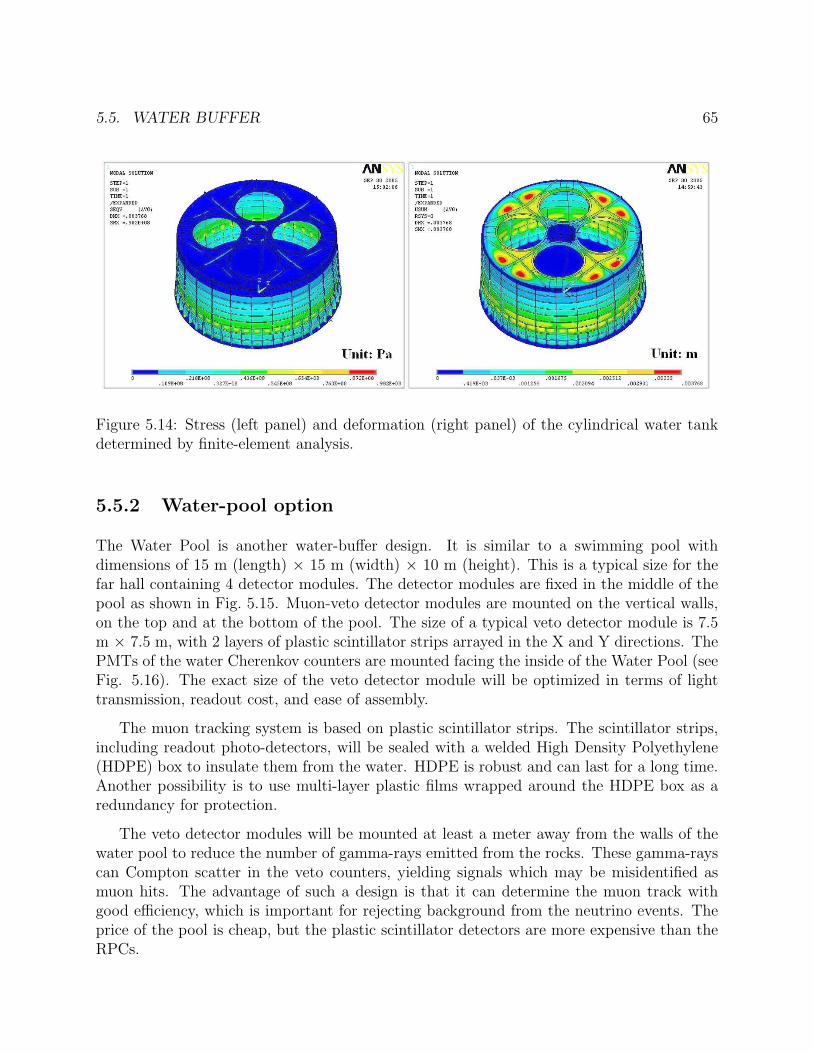
5.5. WATER BUFFER 65
Figure 5.14: Stress (left panel) and deformation (right panel) of the cylindrical water tankdetermined by finite-element analysis.
5.5.2 Water-pool option
The Water Pool is another water-buffer design. It is similar to a swimming pool withdimensions of 15 m (length) × 15 m (width) × 10 m (height). This is a typical size for thefar hall containing 4 detector modules. The detector modules are fixed in the middle of thepool as shown in Fig. 5.15. Muon-veto detector modules are mounted on the vertical walls,on the top and at the bottom of the pool. The size of a typical veto detector module is 7.5m × 7.5 m, with 2 layers of plastic scintillator strips arrayed in the X and Y directions. ThePMTs of the water Cherenkov counters are mounted facing the inside of the Water Pool (seeFig. 5.16). The exact size of the veto detector module will be optimized in terms of lighttransmission, readout cost, and ease of assembly.
The muon tracking system is based on plastic scintillator strips. The scintillator strips,including readout photo-detectors, will be sealed with a welded High Density Polyethylene(HDPE) box to insulate them from the water. HDPE is robust and can last for a long time.Another possibility is to use multi-layer plastic films wrapped around the HDPE box as aredundancy for protection.
The veto detector modules will be mounted at least a meter away from the walls of thewater pool to reduce the number of gamma-rays emitted from the rocks. These gamma-rayscan Compton scatter in the veto counters, yielding signals which may be misidentified asmuon hits. The advantage of such a design is that it can determine the muon track withgood efficiency, which is important for rejecting background from the neutrino events. Theprice of the pool is cheap, but the plastic scintillator detectors are more expensive than theRPCs.
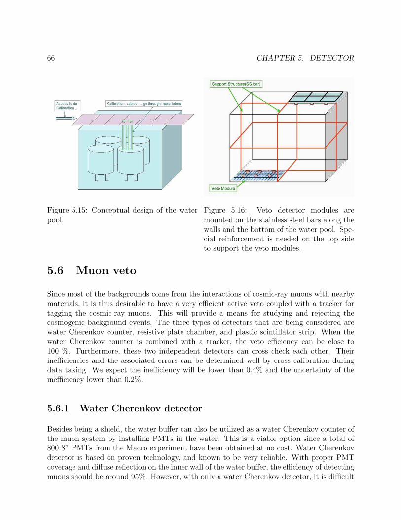
66 CHAPTER 5. DETECTOR
Figure 5.15: Conceptual design of the waterpool.
Figure 5.16: Veto detector modules aremounted on the stainless steel bars along thewalls and the bottom of the water pool. Spe-cial reinforcement is needed on the top sideto support the veto modules.
5.6 Muon veto
Since most of the backgrounds come from the interactions of cosmic-ray muons with nearbymaterials, it is thus desirable to have a very efficient active veto coupled with a tracker fortagging the cosmic-ray muons. This will provide a means for studying and rejecting thecosmogenic background events. The three types of detectors that are being considered arewater Cherenkov counter, resistive plate chamber, and plastic scintillator strip. When thewater Cherenkov counter is combined with a tracker, the veto efficiency can be close to100 %. Furthermore, these two independent detectors can cross check each other. Theirinefficiencies and the associated errors can be determined well by cross calibration duringdata taking. We expect the inefficiency will be lower than 0.4% and the uncertainty of theinefficiency lower than 0.2%.
5.6.1 Water Cherenkov detector
Besides being a shield, the water buffer can also be utilized as a water Cherenkov counter ofthe muon system by installing PMTs in the water. This is a viable option since a total of800 8” PMTs from the Macro experiment have been obtained at no cost. Water Cherenkovdetector is based on proven technology, and known to be very reliable. With proper PMTcoverage and diffuse reflection on the inner wall of the water buffer, the efficiency of detectingmuons should be around 95%. However, with only a water Cherenkov detector, it is difficult
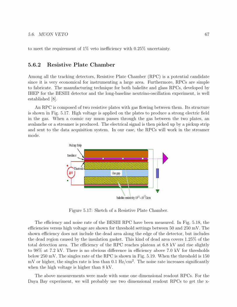
5.6. MUON VETO 67
to meet the requirement of 1% veto inefficiency with 0.25% uncertainty.
5.6.2 Resistive Plate Chamber
Among all the tracking detectors, Resistive Plate Chamber (RPC) is a potential candidatesince it is very economical for instrumenting a large area. Furthermore, RPCs are simpleto fabricate. The manufacturing technique for both bakelite and glass RPCs, developed byIHEP for the BESIII detector and the long-baseline neutrino-oscillation experiment, is wellestablished [8].
An RPC is composed of two resistive plates with gas flowing between them. Its structureis shown in Fig. 5.17. High voltage is applied on the plates to produce a strong electric fieldin the gas. When a cosmic ray muon passes through the gas between the two plates, anavalanche or a streamer is produced. The electrical signal is then picked up by a pickup stripand sent to the data acquisition system. In our case, the RPCs will work in the streamermode.
Figure 5.17: Sketch of a Resistive Plate Chamber.
The efficiency and noise rate of the BESIII RPC have been measured. In Fig. 5.18, theefficiencies versus high voltage are shown for threshold settings between 50 and 250 mV. Theshown efficiency does not include the dead area along the edge of the detector, but includesthe dead region caused by the insulation gasket. This kind of dead area covers 1.25% of thetotal detection area. The efficiency of the RPC reaches plateau at 6.8 kV and rise slightlyto 98% at 7.2 kV. There is no obvious difference in efficiency above 7.0 kV for thresholdsbelow 250 mV. The singles rate of the RPC is shown in Fig. 5.19. When the threshold is 150mV or higher, the singles rate is less than 0.1 Hz/cm2. The noise rate increases significantlywhen the high voltage is higher than 8 kV.
The above measurements were made with some one dimensional readout RPCs. For theDaya Bay experiment, we will probably use two dimensional readout RPCs to get the x-
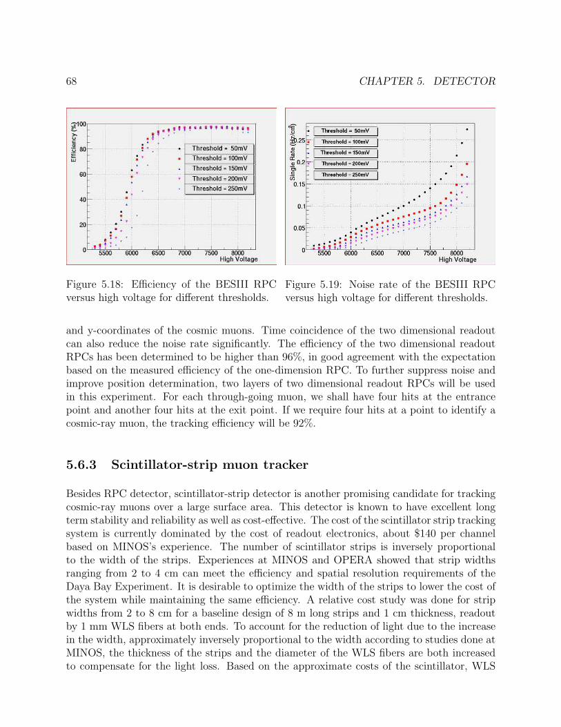
68 CHAPTER 5. DETECTOR
Figure 5.18: Efficiency of the BESIII RPCversus high voltage for different thresholds.
Figure 5.19: Noise rate of the BESIII RPCversus high voltage for different thresholds.
and y-coordinates of the cosmic muons. Time coincidence of the two dimensional readoutcan also reduce the noise rate significantly. The efficiency of the two dimensional readoutRPCs has been determined to be higher than 96%, in good agreement with the expectationbased on the measured efficiency of the one-dimension RPC. To further suppress noise andimprove position determination, two layers of two dimensional readout RPCs will be usedin this experiment. For each through-going muon, we shall have four hits at the entrancepoint and another four hits at the exit point. If we require four hits at a point to identify acosmic-ray muon, the tracking efficiency will be 92%.
5.6.3 Scintillator-strip muon tracker
Besides RPC detector, scintillator-strip detector is another promising candidate for trackingcosmic-ray muons over a large surface area. This detector is known to have excellent longterm stability and reliability as well as cost-effective. The cost of the scintillator strip trackingsystem is currently dominated by the cost of readout electronics, about $140 per channelbased on MINOS’s experience. The number of scintillator strips is inversely proportionalto the width of the strips. Experiences at MINOS and OPERA showed that strip widthsranging from 2 to 4 cm can meet the efficiency and spatial resolution requirements of theDaya Bay Experiment. It is desirable to optimize the width of the strips to lower the cost ofthe system while maintaining the same efficiency. A relative cost study was done for stripwidths from 2 to 8 cm for a baseline design of 8 m long strips and 1 cm thickness, readoutby 1 mm WLS fibers at both ends. To account for the reduction of light due to the increasein the width, approximately inversely proportional to the width according to studies done atMINOS, the thickness of the strips and the diameter of the WLS fibers are both increasedto compensate for the light loss. Based on the approximate costs of the scintillator, WLS
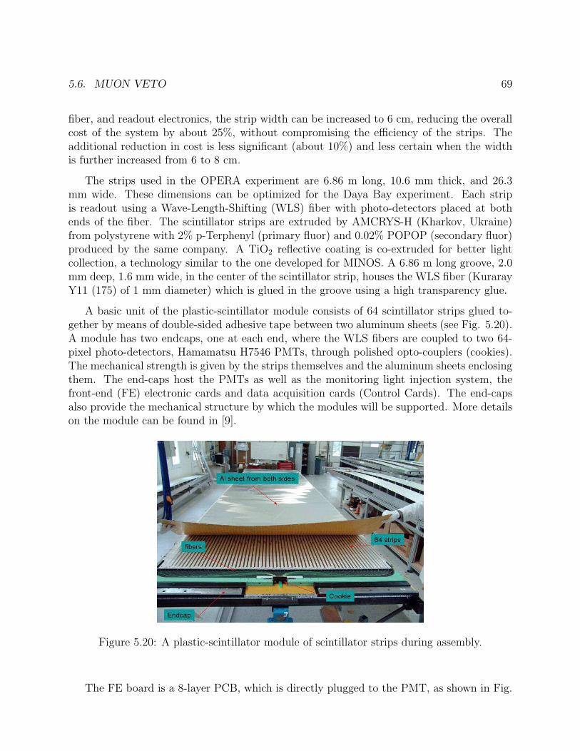
5.6. MUON VETO 69
fiber, and readout electronics, the strip width can be increased to 6 cm, reducing the overallcost of the system by about 25%, without compromising the efficiency of the strips. Theadditional reduction in cost is less significant (about 10%) and less certain when the widthis further increased from 6 to 8 cm.
The strips used in the OPERA experiment are 6.86 m long, 10.6 mm thick, and 26.3mm wide. These dimensions can be optimized for the Daya Bay experiment. Each stripis readout using a Wave-Length-Shifting (WLS) fiber with photo-detectors placed at bothends of the fiber. The scintillator strips are extruded by AMCRYS-H (Kharkov, Ukraine)from polystyrene with 2% p-Terphenyl (primary fluor) and 0.02% POPOP (secondary fluor)produced by the same company. A TiO2 reflective coating is co-extruded for better lightcollection, a technology similar to the one developed for MINOS. A 6.86 m long groove, 2.0mm deep, 1.6 mm wide, in the center of the scintillator strip, houses the WLS fiber (KurarayY11 (175) of 1 mm diameter) which is glued in the groove using a high transparency glue.
A basic unit of the plastic-scintillator module consists of 64 scintillator strips glued to-gether by means of double-sided adhesive tape between two aluminum sheets (see Fig. 5.20).A module has two endcaps, one at each end, where the WLS fibers are coupled to two 64-pixel photo-detectors, Hamamatsu H7546 PMTs, through polished opto-couplers (cookies).The mechanical strength is given by the strips themselves and the aluminum sheets enclosingthem. The end-caps host the PMTs as well as the monitoring light injection system, thefront-end (FE) electronic cards and data acquisition cards (Control Cards). The end-capsalso provide the mechanical structure by which the modules will be supported. More detailson the module can be found in [9].
Figure 5.20: A plastic-scintillator module of scintillator strips during assembly.
The FE board is a 8-layer PCB, which is directly plugged to the PMT, as shown in Fig.
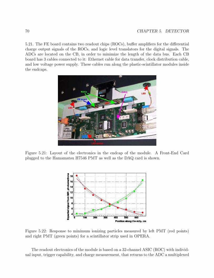
70 CHAPTER 5. DETECTOR
5.21. The FE board contains two readout chips (ROCs), buffer amplifiers for the differentialcharge output signals of the ROCs, and logic level translators for the digital signals. TheADCs are located on the CB, in order to minimize the length of the data bus. Each CBboard has 3 cables connected to it: Ethernet cable for data transfer, clock distribution cable,and low voltage power supply. These cables run along the plastic-scintillator modules insidethe endcaps.
Figure 5.21: Layout of the electronics in the endcap of the module. A Front-End Cardplugged to the Hamamatsu H7546 PMT as well as the DAQ card is shown.
Figure 5.22: Response to minimum ionizing particles measured by left PMT (red points)and right PMT (green points) for a scintillator strip used in OPERA.
The readout electronics of the module is based on a 32-channel ASIC (ROC) with individ-ual input, trigger capability, and charge measurement, that returns to the ADC a multiplexed
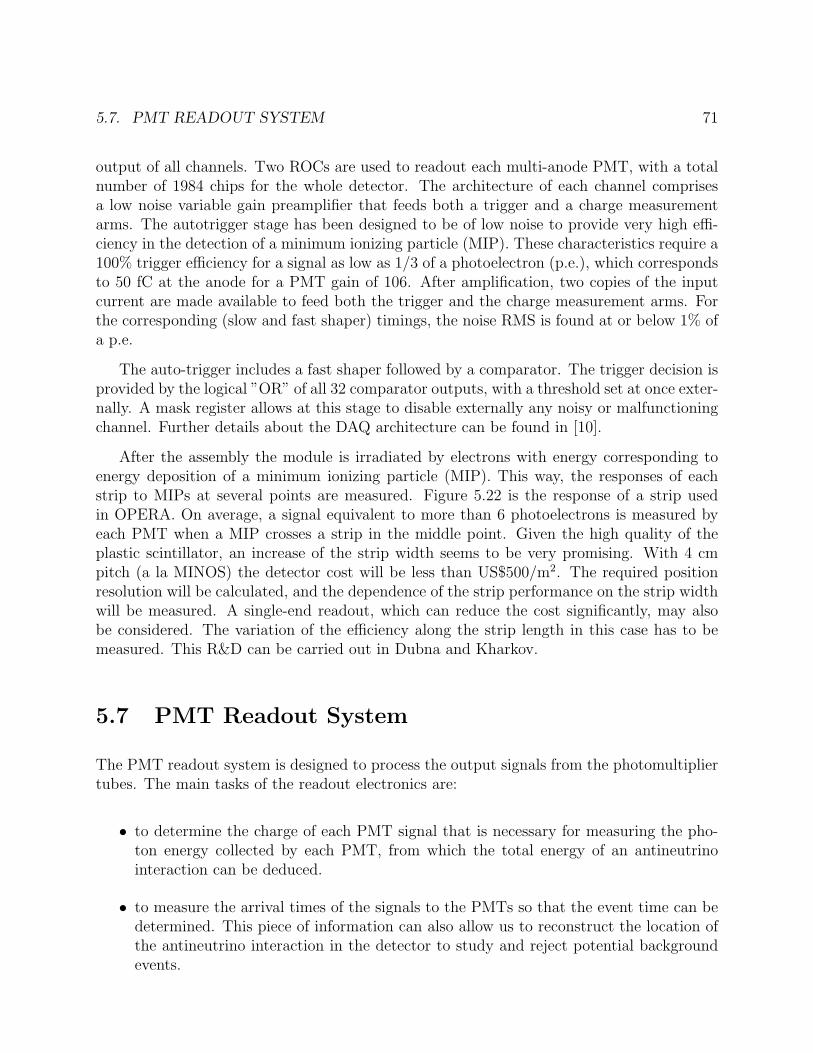
5.7. PMT READOUT SYSTEM 71
output of all channels. Two ROCs are used to readout each multi-anode PMT, with a totalnumber of 1984 chips for the whole detector. The architecture of each channel comprisesa low noise variable gain preamplifier that feeds both a trigger and a charge measurementarms. The autotrigger stage has been designed to be of low noise to provide very high effi-ciency in the detection of a minimum ionizing particle (MIP). These characteristics require a100% trigger efficiency for a signal as low as 1/3 of a photoelectron (p.e.), which correspondsto 50 fC at the anode for a PMT gain of 106. After amplification, two copies of the inputcurrent are made available to feed both the trigger and the charge measurement arms. Forthe corresponding (slow and fast shaper) timings, the noise RMS is found at or below 1% ofa p.e.
The auto-trigger includes a fast shaper followed by a comparator. The trigger decision isprovided by the logical ”OR” of all 32 comparator outputs, with a threshold set at once exter-nally. A mask register allows at this stage to disable externally any noisy or malfunctioningchannel. Further details about the DAQ architecture can be found in [10].
After the assembly the module is irradiated by electrons with energy corresponding toenergy deposition of a minimum ionizing particle (MIP). This way, the responses of eachstrip to MIPs at several points are measured. Figure 5.22 is the response of a strip usedin OPERA. On average, a signal equivalent to more than 6 photoelectrons is measured byeach PMT when a MIP crosses a strip in the middle point. Given the high quality of theplastic scintillator, an increase of the strip width seems to be very promising. With 4 cmpitch (a la MINOS) the detector cost will be less than US$500/m2. The required positionresolution will be calculated, and the dependence of the strip performance on the strip widthwill be measured. A single-end readout, which can reduce the cost significantly, may alsobe considered. The variation of the efficiency along the strip length in this case has to bemeasured. This R&D can be carried out in Dubna and Kharkov.
5.7 PMT Readout System
The PMT readout system is designed to process the output signals from the photomultipliertubes. The main tasks of the readout electronics are:
• to determine the charge of each PMT signal that is necessary for measuring the pho-ton energy collected by each PMT, from which the total energy of an antineutrinointeraction can be deduced.
• to measure the arrival times of the signals to the PMTs so that the event time can bedetermined. This piece of information can also allow us to reconstruct the location ofthe antineutrino interaction in the detector to study and reject potential backgroundevents.
72 CHAPTER 5. DETECTOR
• to provide the energy sum of 16 adjacent channels in real time for the trigger systemto estimate the total energy of an event. The energy sum is the key component of theLevel-1 trigger.
5.7.1 Specifications
• Charge measurement
When a reactor antineutrino interacts in the target, its energy is eventually convertedinto ultraviolet or visible light photons that some of them are transformed into photo-electrons (pe) at the photo-cathodes of the PMTs. For a given PMT, the minimumnumber of photo-electrons is one and, based on Monte Carlo simulation, the maximumnumber of pe is 50 when an antineutrino interaction occurs in the vicinity of theinterface of the Gd-doped liquid scintillator and the gamma catcher. For a through-going cosmic-ray muon, typically 500 pe will be recorded by each PMT. Hence, thedynamic range of the PMT is up to about 500 pe.
Based on the pulse height distribution given in the Hamamatsu data sheet of R5912,the intrinsic energy resolution for a single pe is about 40% when a 410 nm photon isincident on a PMT operating at 1500 V at 25 ◦C. This intrinsic resolution varies fromPMT to PMT as well as the operating conditions of the PMT. The energy thresholdof each PMT will set at about 1/4 pe and the noise contribution from the electronicsis required to be less than 1/10 pe.
The total charge measurement determined by the center-of-gravity method will yieldthe total energy deposited by a signal antineutrino or a background event. This methodwill also reconstruct the event vertex with a precision of several cm based on the pastexperience of Chooz and KamLAND.
• Time measurement
The arrival time of the signal from the PMT will be measured relative to a commonstop signal, for example, the Level-1 trigger.
The rise time of the PMT signal is about 2-3 ns and the time walk of the inherent risingedge of the PMT signal is about 1 ns. Due to the dispersion of the signal cable, therising edge of the signal at the input of the readout module will be smeared dependingon the quality and the length of the signal cable. The design goal for the time resolutionof a single channel is about 0.5 ns or better.
The dynamic range of the time measurement depends on the latency of the level-1trigger and the maximum time difference between the earliest and the latest arrival oflight for a given PMT. The range is chosen to be from 0 to 500 ns.
Since the antineutrino event is a coincidence of a prompt and a delayed sub-event, thesub-event time is a crucial parameter to be determined. This time is a weighted average
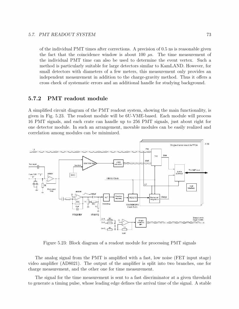
5.7. PMT READOUT SYSTEM 73
of the individual PMT times after corrections. A precision of 0.5 ns is reasonable giventhe fact that the coincidence window is about 100 µs. The time measurement ofthe individual PMT time can also be used to determine the event vertex. Such amethod is particularly suitable for large detectors similar to KamLAND. However, forsmall detectors with diameters of a few meters, this measurement only provides anindependent measurement in addition to the charge-gravity method. Thus it offers across check of systematic errors and an additional handle for studying background.
5.7.2 PMT readout module
A simplified circuit diagram of the PMT readout system, showing the main functionality, isgiven in Fig. 5.23. The readout module will be 6U-VME-based. Each module will process16 PMT signals, and each crate can handle up to 256 PMT signals, just about right forone detector module. In such an arrangement, movable modules can be easily realized andcorrelation among modules can be minimized.
Figure 5.23: Block diagram of a readout module for processing PMT signals
The analog signal from the PMT is amplified with a fast, low noise (FET input stage)video amplifier (AD8021). The output of the amplifier is split into two branches, one forcharge measurement, and the other one for time measurement.
The signal for the time measurement is sent to a fast discriminator at a given thresholdto generate a timing pulse, whose leading edge defines the arrival time of the signal. A stable
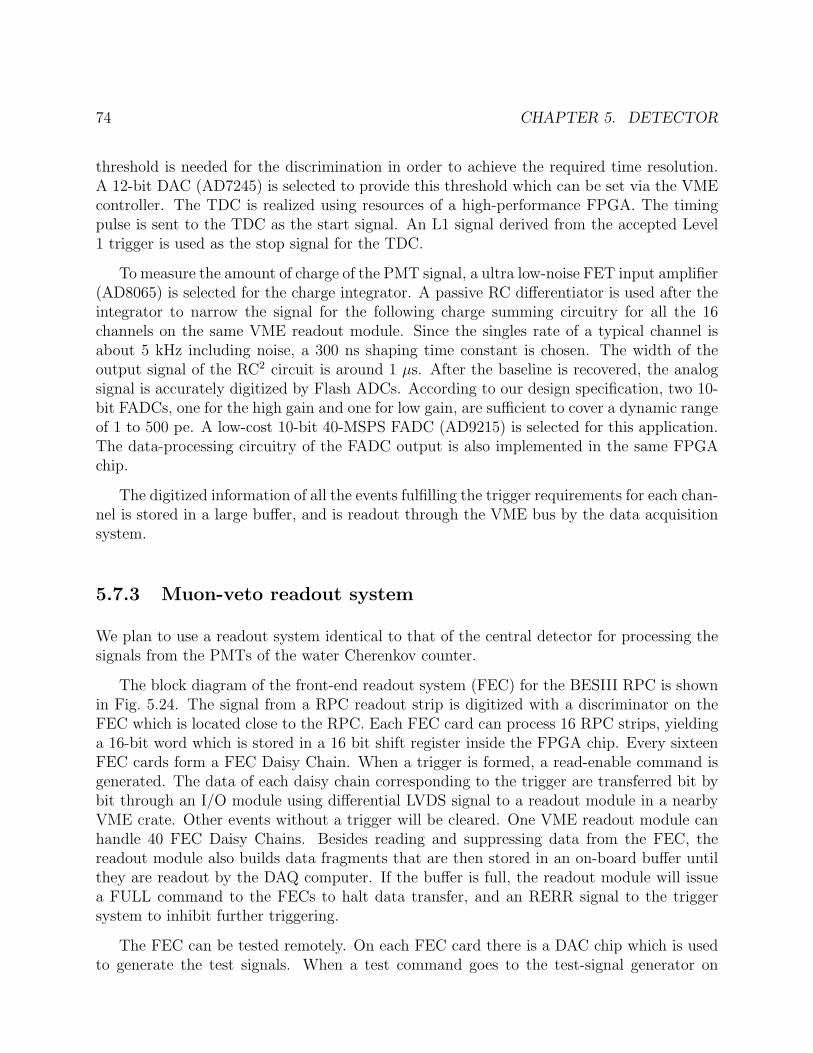
74 CHAPTER 5. DETECTOR
threshold is needed for the discrimination in order to achieve the required time resolution.A 12-bit DAC (AD7245) is selected to provide this threshold which can be set via the VMEcontroller. The TDC is realized using resources of a high-performance FPGA. The timingpulse is sent to the TDC as the start signal. An L1 signal derived from the accepted Level1 trigger is used as the stop signal for the TDC.
To measure the amount of charge of the PMT signal, a ultra low-noise FET input amplifier(AD8065) is selected for the charge integrator. A passive RC differentiator is used after theintegrator to narrow the signal for the following charge summing circuitry for all the 16channels on the same VME readout module. Since the singles rate of a typical channel isabout 5 kHz including noise, a 300 ns shaping time constant is chosen. The width of theoutput signal of the RC2 circuit is around 1 µs. After the baseline is recovered, the analogsignal is accurately digitized by Flash ADCs. According to our design specification, two 10-bit FADCs, one for the high gain and one for low gain, are sufficient to cover a dynamic rangeof 1 to 500 pe. A low-cost 10-bit 40-MSPS FADC (AD9215) is selected for this application.The data-processing circuitry of the FADC output is also implemented in the same FPGAchip.
The digitized information of all the events fulfilling the trigger requirements for each chan-nel is stored in a large buffer, and is readout through the VME bus by the data acquisitionsystem.
5.7.3 Muon-veto readout system
We plan to use a readout system identical to that of the central detector for processing thesignals from the PMTs of the water Cherenkov counter.
The block diagram of the front-end readout system (FEC) for the BESIII RPC is shownin Fig. 5.24. The signal from a RPC readout strip is digitized with a discriminator on theFEC which is located close to the RPC. Each FEC card can process 16 RPC strips, yieldinga 16-bit word which is stored in a 16 bit shift register inside the FPGA chip. Every sixteenFEC cards form a FEC Daisy Chain. When a trigger is formed, a read-enable command isgenerated. The data of each daisy chain corresponding to the trigger are transferred bit bybit through an I/O module using differential LVDS signal to a readout module in a nearbyVME crate. Other events without a trigger will be cleared. One VME readout module canhandle 40 FEC Daisy Chains. Besides reading and suppressing data from the FEC, thereadout module also builds data fragments that are then stored in an on-board buffer untilthey are readout by the DAQ computer. If the buffer is full, the readout module will issuea FULL command to the FECs to halt data transfer, and an RERR signal to the triggersystem to inhibit further triggering.
The FEC can be tested remotely. On each FEC card there is a DAC chip which is usedto generate the test signals. When a test command goes to the test-signal generator on
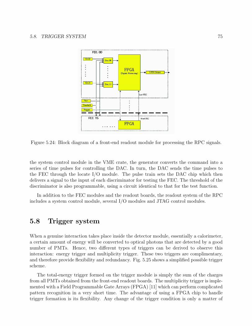
5.8. TRIGGER SYSTEM 75
Figure 5.24: Block diagram of a front-end readout module for processing the RPC signals.
the system control module in the VME crate, the generator converts the command into aseries of time pulses for controlling the DAC. In turn, the DAC sends the time pulses tothe FEC through the locate I/O module. The pulse train sets the DAC chip which thendelivers a signal to the input of each discriminator for testing the FEC. The threshold of thediscriminator is also programmable, using a circuit identical to that for the test function.
In addition to the FEC modules and the readout boards, the readout system of the RPCincludes a system control module, several I/O modules and JTAG control modules.
5.8 Trigger system
When a genuine interaction takes place inside the detector module, essentially a calorimeter,a certain amount of energy will be converted to optical photons that are detected by a goodnumber of PMTs. Hence, two different types of triggers can be derived to observe thisinteraction: energy trigger and multiplicity trigger. These two triggers are complimentary,and therefore provide flexibility and redundancy. Fig. 5.25 shows a simplified possible triggerscheme.
The total-energy trigger formed on the trigger module is simply the sum of the chargesfrom all PMTs obtained from the front-end readout boards. The multiplicity trigger is imple-mented with a Field Programmable Gate Arrays (FPGA) [11] which can perform complicatedpattern recognition in a very short time. The advantage of using a FPGA chip to handletrigger formation is its flexibility. Any change of the trigger condition is only a matter of
76 CHAPTER 5. DETECTOR
Figure 5.25: A simplified trigger scheme
modifying the software that can be downloaded to the FPGA on board easily. Based on ourprevious experience at the Palo Verde [12] and the KamLAND experiments, this technologycan provide satisfactory performance in terms of speed, reliability and complexity.
The 200 MHz FADC on the trigger module has the following functionality:
• provides a cross check of the trigger performance of the FPGA.
• measures the trigger threshold continuously without the need of taking special runs.
• measures the pulse shape that provides an additional handle for rejecting background.
• measures virtually an infinite number of hits during the DAQ dead-time providing anexcellent monitor against the multi-neutron background.
We plan to have a trigger threshold of energy less than 0.7 MeV in order to reach theoff-line threshold for physics of 0.9 MeV. At such a low energy threshold, this trigger will bedominated by background originated from natural radioactivity in the environment, whichis less than 50 Hz based on Monte Carlo simulation, and the dark current of the PMTs, eachrunning at about 4 kHz at 25◦C typically. Using a multiplicity threshold of about 16, thetotal trigger rate would be less than 100 Hz with a 100 ns window.
The time-correlation between simple events, such as electron antineutrino events will bereconstructed off-line. In this way we can easily measure the random correlated background

5.9. CALIBRATION 77
and it is always possible to have a correlated-event trigger if it is necessary due to physicsinterest or too high a background rate.
The muon veto system will have its own trigger. The presence of a muon going throughthe experimental hall can be tagged with a multiplicity trigger based on the number ofstruck PMTs of the water Cherenkov counter. Similarly, if scintillator strips are used totrack muons, the strips can also be utilized to form a muon trigger. The muon triggerscan either serve as a tag or launch a delay trigger looking for activities inside the centraldetector after the passing of a muon, allowing us to study muon-induced background indetail. Information of the muon system along with the central detector will be digitizedwhen a muon-related trigger is satisfied. The time difference between the central detectorand the muon trigger will be recorded.
Each experimental hall will be equipped with an independent DAQ system controlled bya local clock which is synchronized to a master clock for the entire experiment. The localclock will determine the event time for both the veto and the central detector. Furthermore,to minimize correlation among the detector modules, each central detector module will haveits own trigger board and VME crate for data acquisition.
5.9 Calibration
To determine θ13 to high precision, it is essential to understand the performance of thecomplicated antineutrino detector very well. Although every effort is made during the con-struction to ensure all the detector modules to be identical, higher-order small differencesin responses among the detectors are difficult to avoid. These minute differences can leadto slight distortion in the measured energy spectra of the antineutrinos. Without correc-tions, the distorted spectrum may mimic the oscillation effect. The goal of calibration is tomap out these small variations, and introduce the necessary corrections. This will requireemploying many different means to establish the gain and relative timing of each photomul-tiplier tube, the energy response and the energy scale of each detector module. Furthermore,the stability of the detector performance must be monitored regularly throughout the entiredata-collection period.
It is a common practice to utilize three different types of calibration systems to calibrateand monitor the behavior of the detector [13]:
• LED system for calibrating and monitoring the stability of gain of photomultipliertubes.
• Laser system for timing calibration.
• Encapsulated radioactive sources for calibrating the absolute energy scale, and theposition-dependent energy response of the detector.
78 CHAPTER 5. DETECTOR
5.9.1 LED system
The photomultiplier tubes can be calibrated using a stable uniform light source to establishthe gain. The gain stability can also be monitored frequently using the same light source.In addition, the dynamical response of the photomultiplier tubes generally necessitates anextrapolation over two orders of magnitude in light intensity, usually achieved by light in-jection using a powerful laser. Recently, generic small size ultra bright LEDs are readilyavailable. This is a cheaper alternative to the laser system.
The emission spectrum of the LED should be compatible to that of the liquid scintillator.The intensity of the LED is controlled by driving the LED with a nominal square pulse thathas an adjustable width and voltage amplitude. Light from the LED can be injected to eachphotomultiplier tube by routing an optical fiber from a distribution system. Alternatively,light can be guided down a thin light-insulated fiber to a small translucent sphere positionedat the center of the detector. Light will then uniformly illuminate the fiducial volume of thedetector.
5.9.2 Laser system
The propagation time of a photomultiplier tubes in general varies from tube to tube. Thedifference in the propagation time can be due to different cable length, or transit time. It isessential to obtain accurate relative timing of the PMT signals for precise reconstruction ofthe vertex position.
A laser flasher with a mixer ball can be used to adjust timing and to measure chargedependence. Light pulses from the laser are injected into the light mixer ball at the detectorcenter through an optical fiber, and isotropic light is emitted by the mixer ball. The light isdetected by all the photomultiplier tubes. The time difference between each PMT and thereference PMT is then measured. The intensity of the laser can be changed by a trigger andis monitored with a 2-inch PMT.
5.9.3 Radioactive sources
The absolute energy scale of the experiment can be established by calibrating the modulesby a set of radioactive sources along with detailed Monte Carlo simulation. In addition, thelinearity of the energy scale in the region of interest can be investigated as well. The non-linearity is caused by Cherenkov threshold effect, quenching effect, noise hit, and inefficiencyof detecting single photoelectrons. A combined radioactive source emitting a gamma rayand a neutron can be employed to estimate the efficiency of detecting reactor antineutrinossince the signal topology of the artificial source is similar to that of the inverse beta decayreaction.
5.9. CALIBRATION 79
The radioactive sources 68Ge, 22Na, 24Na, 65Zn, 60Co, and Am-Be will be used for energycalibration between 1 and 8 MeV. Two gamma-rays, each with 0.511 MeV of energy, areemitted from the positron annihilation in the 68Ge source. One gamma-ray of 1.116 MeV isemitted from the 65Zn source. A 1.173 MeV gamma-ray and a 1.332 MeV gamma-ray areemitted at same time from the 60Co source. The energy scale at 7.652 MeV is calibratedby the gamma-rays emitted by the Am-Be source. The monochromatic gamma-ray with anenergy of 2.22 MeV coming from the muon-induced neutron captured by hydrogen in theliquid scintillator can be utilized for calibration as well. Furthermore, the 4.947 MeV gamma-ray originating from muon-induced neutron captured by carbon in the liquid scintillator willalso be used.
It should be noted that there is a difference between the real energies of the particlesand the measured ones (quenching effect). The deficit of scintillation light [14] depends onthe type of particle (in our case we have positron and two annihilation gamma-rays). In theChooz experiment the difference between the real and measured energies was:
• ∆(2× 0.511 MeV annihilation gammas) = 125.6 keV,
• ∆(2.225 MeV gamma-ray from np-capture) = 67.9 keV,
• ∆(1.27 MeV gamma-ray from 22Na-source) = 65.9 keV,
• ∆(2.29 MeV gamma-ray from 22Na -source) = 191.5 keV,
• ∆( 8MeV gamma-rays from n-Gd-capture) = 189 keV.
This effect should be investigated and be taken into account in the energy calibration.A method of measuring the quenching effect at the low-background condition is to use a22Na source. The idea is to use the positron from the source as an independent trigger andto measure the energy of the 1.27 MeV gamma-ray and two annihilation gamma-rays. Thisapproach will give us additional calibration information, practically avoiding the externalbackground and accidental coincidence. Another method is to use a small spontaneousfission 252Cf source placed at the center of the detector. The source generates a continuousenergy spectrum due to neutron recoils and the prompt fission gamma-rays. Any deviationfrom unity for the ratio of spectra measured at two detectors can be used to calculate therelative corrections.
The absolute efficiency of detecting a neutron can be determined by radioactive sourceswith tagging capability. For instance, with ≈50% branching fraction of the α+9Be reactionwhere the α is emitted from Am decay, the neutron emitted by an Am-Be source can betagged by the accompanying 4.43 MeV gamma-ray. Another possible candidate is 252Cf whichemits on average 3.77 neutrons per fission. The distribution of the number of neutronsemitted in a fission of 252Cf is well known up to a multiplicity of 10 [15]. The efficiencyof detecting a neutron can be determined again by tagging the prompt gamma-rays from
80 CHAPTER 5. DETECTOR
each fission along with the emitted neutrons. The resulting probability Q(n) of observed nneutrons for i emitted (n < i) is just
Q(n) =∑
i
P (i)i!
n!(i− n)!εn(1− ε)i−n (5.1)
where P(i) are constants, and ε is the detection efficiency. The probability Q(n) dependson the operational conditions of a given detector such as the time window and the energythreshold of detecting the Gd-captured neutron. The absolute efficiency of detecting aneutron can be determined by fitting the observed multiplicity distribution of neutron toEquation 5.1. There is weak dependence between the number of emitted neutrons and theprompt gamma-ray energy. The lower the energy of the gamma-ray is, the higher the meanvalue of the emitted neutrons will be. Thus, the loss of low-energy gamma-rays leads to thedistortion of the neutron multiplicity distribution. To avoid this effect we will analyze theneutron multiplicity distribution obtained with a prompt-gamma trigger beginning from asingle neutron. Combining different measurements and Monte Carlo simulation it is possibleto get a precision of better than 0.5% for the absolute efficiency of detecting neutrons.
Each radioactive source is encapsulated in a small container to prevent any potentialcontamination of the ultra-pure liquid scintillator. The assembly is kept in an extremelyclean environment that is sealed off from radon penetration. The radioactive source will bedeployed to the target volume and the gamma catcher in turn along different vertical axesof the detector by attaching it to a string which is lowered into the detector via a controlledmotor. The position of the source inside detector is determined by the length of the stringin the detector.
Bibliography
[1] R. Brun, F. Carminati, GEANT Detector Description and Simulation Tool, CERNProgram Library Long Writeup W5013, September 1993.
[2] C. Zeitnitz and T. A. Gabriel, The GEANT-Calor interface user’s guide. September,2001.
[3] L. H. Miller, Ph.D thesis (unpublished), Stanford University (2000).
[4] F. Boehm et al. (Palo Verde Collaboration), Phys. Rev. Lett. 84, 3764 (2000) [arXiv:hep-ex/9912050]; Phys. Rev. D62, 072002 (2000) [arXiv:hep-ex/0003022]; Phys. Rev. D64,112001 (2001) [arXiv:hep-ex/0107009]; A. Piepke et al., Nucl. Instr. and meth. A432,392 (1999).
[5] M. Apollonio et al. (Chooz Collaboration), Phys. Lett. B420, 397 (1998); Phys. Lett.B466, 415 (1999); Eur. Phys. J. C27, 331 (2003).
[6] K. Eguchi et al. (KamLAND collaboration), Phys. Rev. Lett. 90, 021802 (2003).
[7] V. M. Novikov, Nucl. Instr. and Meth. A366, 413 (1995).
[8] J.W. Zhang et al, High Energy Phys. and Nucl. Phys., 27, 615 (2003).
[9] OPERA proposal, ,”An appearance experiment to search for νµ ↔ ντ oscillations in theCNGS beam”, CERN/SPSC 2000-028, SPSC/P318, LNGS P25/2000, July 10, 2000.
[10] C. Girerd et al., ethernet network based DAQ and smart sensors for the OPERA long-baseline neutrino experiment, LYCEN 2000-109, IEEE Nuclear Science Symposium andNuclear Imaging Conference, Lyon, October 15-20, 2000.
[11] For example, Virtex chip from Xilinx Corp. See http://www.xilinx.com.
[12] G. Gratta et al., Nucl. Instr. and Meth. A400, 54 (1997).
[13] L. Mikaelyan, Nucl. Phys. B (Proc. Suppl.) 91, 120 (2001), (hep-ex/0008046); V.Martemianov et al., Phys. Atom. Nucl. 66, 1934 (2003), (hep-ex/0211070).
81

82 BIBLIOGRAPHY
[14] J.B. Birks, Phys. Soc. A64, 874 (1951).
[15] Yu.V. Kozlov, V.P. Martemyanov, V.N. Vyrodov et al. J. of Nucl. Phys. 36 3(9), 587(1982); J.W. Boldeman et al. Nucl. Sci. Eng. A 189, 285 (1972).
Chapter 6
Detector Overburden andBackgrounds
For a reactor-based θ13 experiment, the minimization of background will be an importantconsideration in site selection and detector design. In the Daya Bay experiment, the signalevents (inverse beta decay reactions) have a distinct signature of two time-ordered signals:A prompt positron signal (prompt trigger) followed by a neutron-capture signal (delayedtrigger). Backgrounds can be classified into two categories: correlated and uncorrelatedbackgrounds. If a background event is triggered by two signals that come from the samesource, such as those induced by the same cosmic muon, it is a correlated background event.On the other hand, if the two signals come from different sources but satisfy the triggerrequirements by chance, the event is an uncorrelated background.
There are three important sources of backgrounds in the Daya Bay experiment: fastneutrons, 8He/9Li, and natural radioactivity. A fast neutron produced by cosmic muons inthe surrounding rocks or the detector can produce a signal mimicking the inverse beta decayreaction in the detector: the recoil proton generates the prompt signal and the capture of thethermalized neutron provides the delayed signal. The 8He/9Li isotopes produced by cosmicmuons have substantial beta-neutron decay branching fractions, 16% for 8He and 49.5% for9Li. The beta energy of the beta-neutron cascade overlaps the positron signal of neutrinoevents, simulating the prompt signal, and the neutron emission forms the delayed signal.Fast neutrons and 8He/9Li isotopes create correlated backgrounds since both the promptand delayed signals are from the same single parent muon. Some neutrons produced bycosmic muons are captured in the detector without proton recoil energy. A single neutroncapture signal has some probability to fall accidentally within the time window of a precedingsignal due to natural radioactivity in the detector, producing an accidental background. Inthis case, the prompt and delayed signals are from different sources, forming an uncorrelatedbackground.
All the three major backgrounds are related to cosmic muons whose flux cannot be easily
83
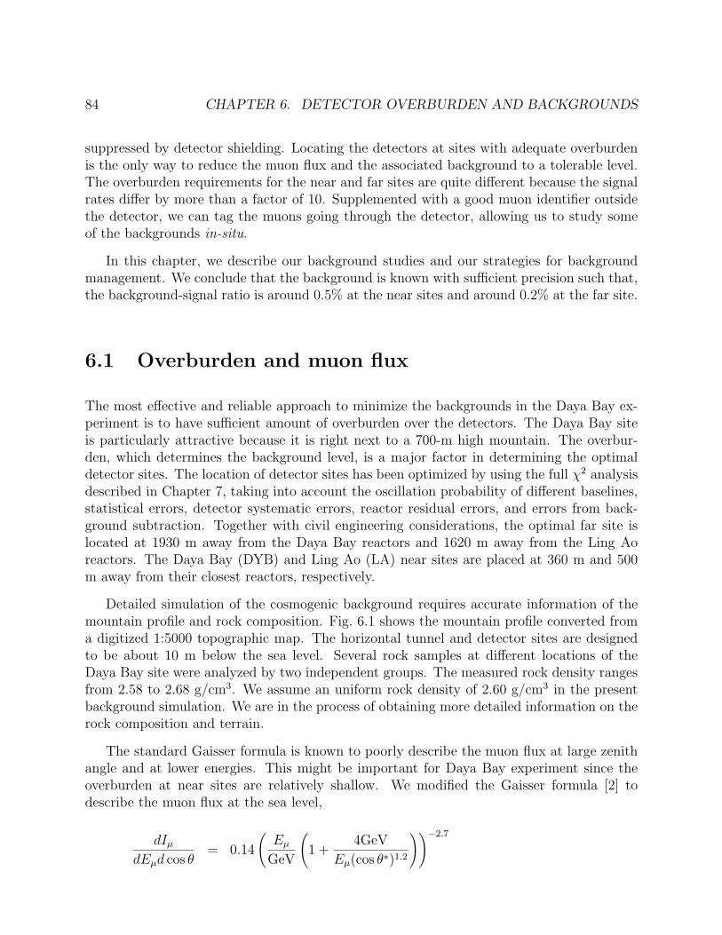
84 CHAPTER 6. DETECTOR OVERBURDEN AND BACKGROUNDS
suppressed by detector shielding. Locating the detectors at sites with adequate overburdenis the only way to reduce the muon flux and the associated background to a tolerable level.The overburden requirements for the near and far sites are quite different because the signalrates differ by more than a factor of 10. Supplemented with a good muon identifier outsidethe detector, we can tag the muons going through the detector, allowing us to study someof the backgrounds in-situ.
In this chapter, we describe our background studies and our strategies for backgroundmanagement. We conclude that the background is known with sufficient precision such that,the background-signal ratio is around 0.5% at the near sites and around 0.2% at the far site.
6.1 Overburden and muon flux
The most effective and reliable approach to minimize the backgrounds in the Daya Bay ex-periment is to have sufficient amount of overburden over the detectors. The Daya Bay siteis particularly attractive because it is right next to a 700-m high mountain. The overbur-den, which determines the background level, is a major factor in determining the optimaldetector sites. The location of detector sites has been optimized by using the full χ2 analysisdescribed in Chapter 7, taking into account the oscillation probability of different baselines,statistical errors, detector systematic errors, reactor residual errors, and errors from back-ground subtraction. Together with civil engineering considerations, the optimal far site islocated at 1930 m away from the Daya Bay reactors and 1620 m away from the Ling Aoreactors. The Daya Bay (DYB) and Ling Ao (LA) near sites are placed at 360 m and 500m away from their closest reactors, respectively.
Detailed simulation of the cosmogenic background requires accurate information of themountain profile and rock composition. Fig. 6.1 shows the mountain profile converted froma digitized 1:5000 topographic map. The horizontal tunnel and detector sites are designedto be about 10 m below the sea level. Several rock samples at different locations of theDaya Bay site were analyzed by two independent groups. The measured rock density rangesfrom 2.58 to 2.68 g/cm3. We assume an uniform rock density of 2.60 g/cm3 in the presentbackground simulation. We are in the process of obtaining more detailed information on therock composition and terrain.
The standard Gaisser formula is known to poorly describe the muon flux at large zenithangle and at lower energies. This might be important for Daya Bay experiment since theoverburden at near sites are relatively shallow. We modified the Gaisser formula [2] todescribe the muon flux at the sea level,
dIµ
dEµd cos θ= 0.14
(Eµ
GeV
(1 +
4GeV
Eµ(cos θ∗)1.2
))−2.7
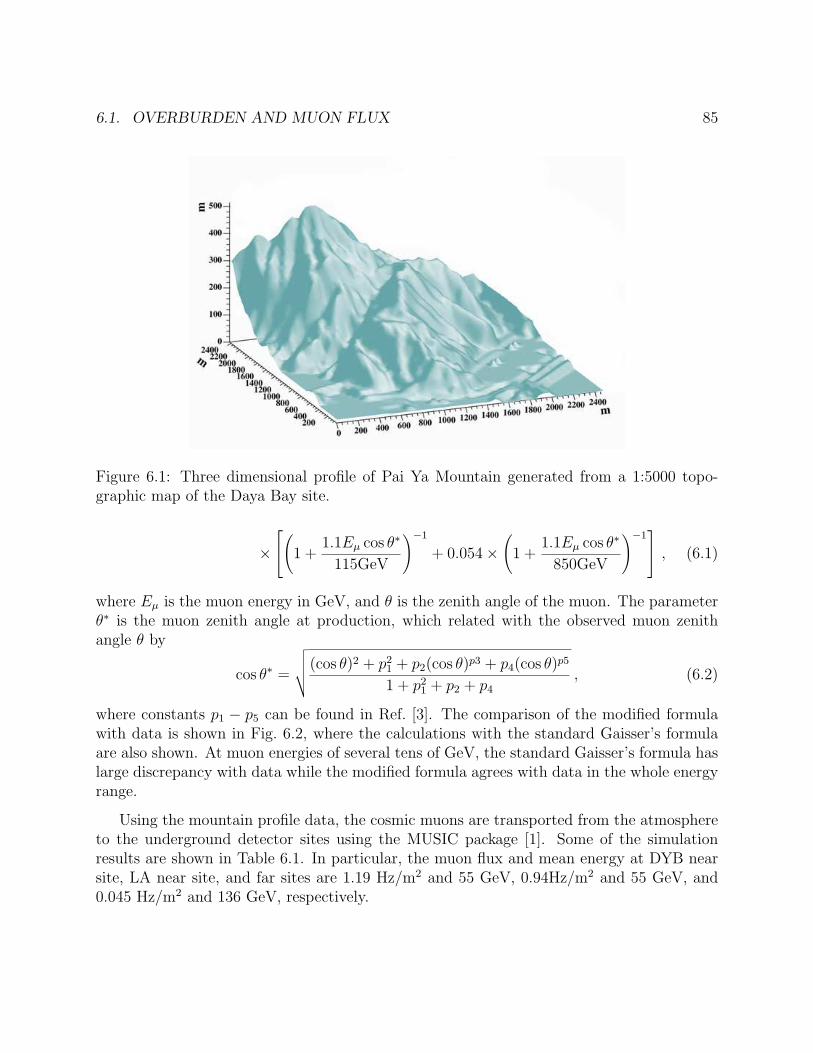
6.1. OVERBURDEN AND MUON FLUX 85
Figure 6.1: Three dimensional profile of Pai Ya Mountain generated from a 1:5000 topo-graphic map of the Daya Bay site.
×
(1 +
1.1Eµ cos θ∗
115GeV
)−1
+ 0.054×(
1 +1.1Eµ cos θ∗
850GeV
)−1 , (6.1)
where Eµ is the muon energy in GeV, and θ is the zenith angle of the muon. The parameterθ∗ is the muon zenith angle at production, which related with the observed muon zenithangle θ by
cos θ∗ =
√√√√(cos θ)2 + p21 + p2(cos θ)p3 + p4(cos θ)p5
1 + p21 + p2 + p4
, (6.2)
where constants p1 − p5 can be found in Ref. [3]. The comparison of the modified formulawith data is shown in Fig. 6.2, where the calculations with the standard Gaisser’s formulaare also shown. At muon energies of several tens of GeV, the standard Gaisser’s formula haslarge discrepancy with data while the modified formula agrees with data in the whole energyrange.
Using the mountain profile data, the cosmic muons are transported from the atmosphereto the underground detector sites using the MUSIC package [1]. Some of the simulationresults are shown in Table 6.1. In particular, the muon flux and mean energy at DYB nearsite, LA near site, and far sites are 1.19 Hz/m2 and 55 GeV, 0.94Hz/m2 and 55 GeV, and0.045 Hz/m2 and 136 GeV, respectively.
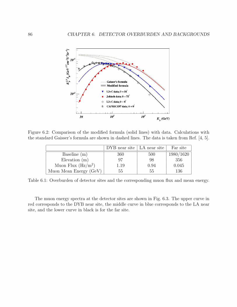
86 CHAPTER 6. DETECTOR OVERBURDEN AND BACKGROUNDS
Figure 6.2: Comparison of the modified formula (solid lines) with data. Calculations withthe standard Gaisser’s formula are shown in dashed lines. The data is taken from Ref. [4, 5].
DYB near site LA near site Far site
Baseline (m) 360 500 1980/1620Elevation (m) 97 98 356
Muon Flux (Hz/m2) 1.19 0.94 0.045Muon Mean Energy (GeV) 55 55 136
Table 6.1: Overburden of detector sites and the corresponding muon flux and mean energy.
The muon energy spectra at the detector sites are shown in Fig. 6.3. The upper curve inred corresponds to the DYB near site, the middle curve in blue corresponds to the LA nearsite, and the lower curve in black is for the far site.
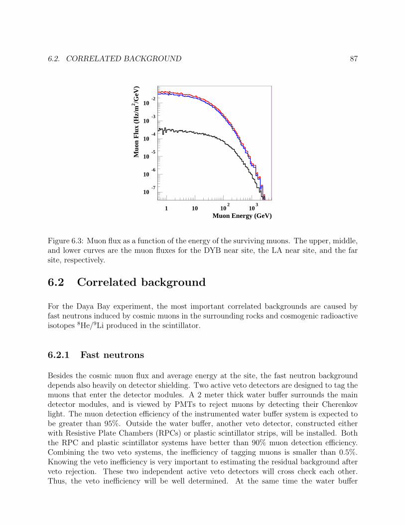
6.2. CORRELATED BACKGROUND 87
10-7
10-6
10-5
10-4
10-3
10-2
1 10 102
103
Muon Energy (GeV)
Muo
n F
lux
(Hz/
m2 /G
eV)
Figure 6.3: Muon flux as a function of the energy of the surviving muons. The upper, middle,and lower curves are the muon fluxes for the DYB near site, the LA near site, and the farsite, respectively.
6.2 Correlated background
For the Daya Bay experiment, the most important correlated backgrounds are caused byfast neutrons induced by cosmic muons in the surrounding rocks and cosmogenic radioactiveisotopes 8He/9Li produced in the scintillator.
6.2.1 Fast neutrons
Besides the cosmic muon flux and average energy at the site, the fast neutron backgrounddepends also heavily on detector shielding. Two active veto detectors are designed to tag themuons that enter the detector modules. A 2 meter thick water buffer surrounds the maindetector modules, and is viewed by PMTs to reject muons by detecting their Cherenkovlight. The muon detection efficiency of the instrumented water buffer system is expected tobe greater than 95%. Outside the water buffer, another veto detector, constructed eitherwith Resistive Plate Chambers (RPCs) or plastic scintillator strips, will be installed. Boththe RPC and plastic scintillator systems have better than 90% muon detection efficiency.Combining the two veto systems, the inefficiency of tagging muons is smaller than 0.5%.Knowing the veto inefficiency is very important to estimating the residual background afterveto rejection. These two independent active veto detectors will cross check each other.Thus, the veto inefficiency will be well determined. At the same time the water buffer
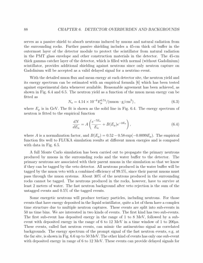
88 CHAPTER 6. DETECTOR OVERBURDEN AND BACKGROUNDS
serves as a passive shield to absorb neutrons induced by muons and natural radiation fromthe surrounding rocks. Further passive shielding includes a 45-cm thick oil buffer in theoutermost layer of the detector module to protect the scintillator from natural radiationin the PMT glass envelope and other construction materials in the detector. The 45-cmthick gamma catcher layer of the detector, which is filled with normal (without Gadolinium)scintillator, provides additional shielding against neutrons since only neutron capture onGadolinium will be accepted as a valid delayed signal for a neutrino event.
With the detailed muon flux and mean energy at each detector site, the neutron yield andits energy spectrum can be estimated with an empirical formula [6] which has been testedagainst experimental data whenever available. Reasonable agreement has been achieved, asshown in Fig. 6.4 and 6.5. The neutron yield as a function of the muon mean energy can befitted as
Nn = 4.14× 10⁻⁶E0.74µ /(muon · g/cm2) , (6.3)
where Eµ is in GeV. The fit is shown as the solid line in Fig. 6.4. The energy spectrum ofneutron is fitted to the empirical function
dN
dEn
= A
(e−7En
En
+ B(Eµ)e−2En
), (6.4)
where A is a normalization factor, and B(Eµ) = 0.52− 0.58 exp(−0.0099Eµ). The empiricalfunction fits well to FLUKA simulation results at different muon energies and is comparedwith data in Fig. 6.5.
A full Monte Carlo simulation has been carried out to propagate the primary neutronsproduced by muons in the surrounding rocks and the water buffer to the detector. Theprimary neutrons are associated with their parent muons in the simulation so that we knowif they can be tagged by the veto detector. All neutrons produced in the water buffer will betagged by the muon veto with a combined efficiency of 99.5%, since their parent muons mustpass through the muon systems. About 30% of the neutrons produced in the surroundingrocks cannot be tagged. The neutrons produced in the rocks, however, have to survive atleast 2 meters of water. The fast neutron background after veto rejection is the sum of theuntagged events and 0.5% of the tagged events.
Some energetic neutrons will produce tertiary particles, including neutrons. For thoseevents that have energy deposited in the liquid scintillator, quite a lot of them have a complextime structure due to multiple neutron captures. These events are split into sub-events in50 ns time bins. We are interested in two kinds of events. The first kind has two sub-events.The first sub-event has deposited energy in the range of 1 to 8 MeV, followed by a sub-event with deposited energy in the range of 6 to 12 MeV in a time window of 1 to 200µs.These events, called fast neutron events, can mimic the antineutrino signal as correlatedbackgrounds. The energy spectrum of the prompt signal of the fast neutron events, e.g. atthe far site, is shown in Fig. 6.6 up to 50 MeV. The other kind of events has only one sub-eventwith deposited energy in range of 6 to 12 MeV. These events can provide delayed signals for

6.2. CORRELATED BACKGROUND 89
Eµ (GeV)
Neu
tro
n y
ield
(n
/µg
cm-2
)
A
B
C
D
E
F
G
10-4
10 102
Figure 6.4: Neutron yield as a functionof mean muon energy. The stars indicateFLUKA simulation results. The solid lineis a fit of the simulation results to a powerlaw in Eq. 6.3. The crosses are data pointstaken from underground experiments at var-ious depths. For details see Ref. [6].
En (MeV)
Eve
nts
/s/M
eV
Nsofte-E/2.1+Nharde-E/39
Our parameterization
Karmen Data
En (MeV)
Eve
nts
/mu
on
/co
un
ter/
MeV LVD Data
Our parameterization
10-4
10-3
10 15 20 25 30 35 40 45 50
10-9
10-8
10-7
10-6
10 102
Figure 6.5: Comparison of measured neu-tron energy spectrum with the empiricalfunction in Eq. 6.4.
the uncorrelated backgrounds. We call them single neutron events. The simulation resultsare listed in Table 6.2.
DYB near site LA near site far site
fast neutron vetoed 57.8 45.6 3.8(/day/module) not vetoed 0.83 0.64 0.08
single neutron vetoed 1365 1070 94.7(/day/module) not vetoed 27.2 21.0 2.1
Table 6.2: Neutron rates in a 20-ton module at the Daya Bay sites. The rows labelled”vetoed” refer to the case where the parent muon track traversed the veto detectors, andthus it could be tagged. Rows labelled ”not vetoed” refer to the case where the muon trackdid not traverse the veto detectors.
90 CHAPTER 6. DETECTOR OVERBURDEN AND BACKGROUNDS
Figure 6.6: The prompt energy spectrum of fast neutron backgrounds at the Daya Bay fardetector. The inset is an expanded view of the spectrum from 1 to 10 MeV.
6.2.2 Cosmogenic 8He/9Li
Cosmic muons, even if they are tagged by the muon identifier, can produce radioactiveisotopes in the detector scintillator which decay by emitting both a beta and a neutron(β-neutron emission isotopes). Some of these so-called cosmogenic radioactive isotopes livelong enough such that their decay cannot be reliably associated with the last vetoed muon.Among them, 8He and 9Li with half-lives of 0.12 s and 0.18 s, respectively, constitute the mostserious correlated background sources. The production cross section of these two isotopeshas been measured with muons at an energy of 190 GeV at CERN [10]. Their combinedcross section is σ(9Li +8 He) = (2.12 ± 0.35)µbarn. Since their lifetimes are so close, it ishard to get their individual cross sections. About 16% of 8He and 49.5% of 9Li will decayby β-neutron emission. Using the muon flux and mean energy given in last section at thesites and an energy dependence of the cross section, σtot(Eµ) ∝ Eα
µ , with α = 0.73, thebackground-to-signal ratio (B/S) is estimated to be around 0.5% for the near sites and 0.2%for the far site, assuming that 49.5% of the isotopes contribute to the backgrounds.
KamLAND experiment measures the isotope background very well by fitting the timesince last muon. The KamLAND detector has an average overburden of 2700 m.w.e. (meter-water-equivalent), resulting in a muon flux of 0.0015 Hz/m2, or 0.2 Hz of cosmic-ray muonsin the detector active volume. The mean time interval of successive muons is 5 seconds, muchlonger than the lifetimes of 9Li/8He. For the Daya Bay experiment, the muon flux is 1.2,0.94, and 0.04 Hz/m2 at the DYB near site, the LA near site, and the far site, respectively.The target volume of a 20 ton detector module has a cross section around 10 m2. Thus themuon rate is around 10 Hz at the near sites, resulting in a mean time interval of successivemuons shorter than the lifetimes of 9Li/8He. With a modified fitting algorithm, we find thatit is still feasible to measure the isotope background in-situ.
From the decay time and β-energy spectra fit, the contribution of 8He relative to that of
6.2. CORRELATED BACKGROUND 91
9Li was determined to be less than 15% at 90% confidence level [11]. Furthermore, the 8Hecontribution can be identified by tagging the double cascade 8He →8 Li →8 Be [13]. In thefollowing we assume that all isotope backgrounds are from 9Li.
The arrival times of the muons are uniformly distributed in time. The time intervalbetween two successive muons t follows the exponential distribution law
fµ(t) =1
Texp(−t/T ), (6.5)
where the time constant T is the mean time interval between successive muons. T = 1/Rµ,where Rµ is the muon rate. The neutrino events are also uniformly distributed in time, andare independent of the muons. The time interval between a neutrino event and the last muonalso follows an exponential distribution law, with a time constant T ′ = 1/(Rµ + Rν), whereRν is the neutrino rate. Since the neutrino rate is 2 ∼ 3 orders of magnitude lower than themuon rate for a typical Daya Bay site, the difference between T ′ and T can be ignored. Theproduction times of 9Li are correlated with the arrival times of the muons. If the muon rateis high, a 9Li is not necessarily produced by the last muon. When summed over all precedingmuons, the probability density function of the time since the last muon t is
fLi(t) =1
λexp(−t/λ) ,
1
λ=
1
τ+
1
T, (6.6)
where τ = 0.258 s is the lifetime of 9Li. The isotope backgrounds can be measured by fittingthe observed distribution to two exponentials, one for neutrino and the other for 9Li. Sincethe 9Li and the neutrino rates are much lower than the muon rate, the probability of twoneutrino-like events falling into the fitting time window is negligible. The muons immediatelyfollowing a neutrino candidate can be simply ignored. It is therefore not necessary to restrictthe fitting time window to the interval between two successive muons.
In the distribution Eq. 6.6, contributions of all preceding muons are averaged and com-bined into the last muon. The fitting can be done with either the least χ2 method or theunbinned maximum likelihood method. Assuming that each neutrino candidate has a prob-ability of b to be a 9Li and 1− b to be a neutrino, the likelihood function is
log L =∑
i
log[b1
λe−ti/λ + (1− b)
1
Te−ti/T
], (6.7)
where ti is time of the i-th neutrino candidate since last muon.
Maximum likelihood fitting can make use of the timing information of preceding muons,instead of using the average effect. It will be useful for lower muon rate, such as at the farsite. The likelihood function can be written as
log L =∑
i
log
b
∑
j
1
τe−tij/τ
e−ti1/T + (1− b)
1
Te−ti1/T
, (6.8)
92 CHAPTER 6. DETECTOR OVERBURDEN AND BACKGROUNDS
where i sums over all neutrino candidates and j sums over all preceding muons of the i-thneutrino candidate. ti1 is the time since last muon and tij is the time since the j-th precedingmuon. In practice, only muons in a 2-second window are summed. This cut-off results in adifference of probability smaller than 10−3.
Precision of the parameter fitting can be estimated for the maximum likelihood methodwhen the sample size is very large. If b ¿ τ/(τ + T ), which is true for all Daya Bay sites,the fitting precision of b in Eq. 6.7 can be approximated as
σb =1√N·√
(1 + τRµ)2 − 1 , (6.9)
where N is total number of neutrino candidates.
To explore the fitting algorithm, we simulated the event sample of the Daya Bay experi-ment for 3 years of running, with neutrinos, muons, and 9Li taken into account. At a givensite, the neutrino events are generated with uniform random numbers in time. The numberof muons is calculated according to the muon rate Rµ at the site. Muons are also gener-ated with uniform random numbers in time. The number of 9Li produced by each muon iscalculated with Poisson statistics. The 9Li yield is of the order of 10−5 per muon. If a 9Liis produced by a muon, its decay time is sampled by the exponential decay law. The twoindependent data sets, one containing neutrino events and the other containing muon and9Li events, are combined and sorted by time for the analysis. In the data sample generation,only time information is stored. The energy spectrum of 9Li events is not taken into account,neither is the muon-energy dependence of the yield of 9Li.
Fig. 6.7 shows the fitting results as a function of muon rate. The background-to-signalratio is fixed at 1%. The total neutrino candidate number is 2.5×10⁵, corresponding to 0.2%statistical error. The data sample generation and fitting were performed 400 times for eachpoint. In Fig. 6.8 the fitting precision is compared to the analytic formula Eq. 6.9 with thesame Monte Carlo samples in Fig. 6.7. The Monte Carlo results of the least χ2 fitting, themaximum likelihood fitting, and the simple analytical estimation are in excellent agreement.
In conclusion, the background-to-signal ratio of isotope background can be measured to∼ 0.3% with two 20-ton modules at the near sites of the Daya Bay experiment and ∼ 0.1%at the far site with four 20-ton modules, with the data sample of three years of running. Thefitting uses time information only. Inclusion of energy and vertex information may improvethe precision.
KamLAND found that around 85% isotope background are produced by shower muons[11]. A 2-second veto of the whole detector is applied at KamLAND to reject the isotopebackground. Around 3% of cosmic muons will cause a shower in the detector. It is unlikelyfor Daya Bay to apply a 2-second veto since the dead time of the near detector will bemore than 50%. If the detector is vetoed for 0.5 s after a shower muon, about 85% isotopebackgrounds caused by shower muons can be rejected. The remaining isotope backgroundwill be around 30%, 15% from non-shower muons and 15% from shower muons. Taking into
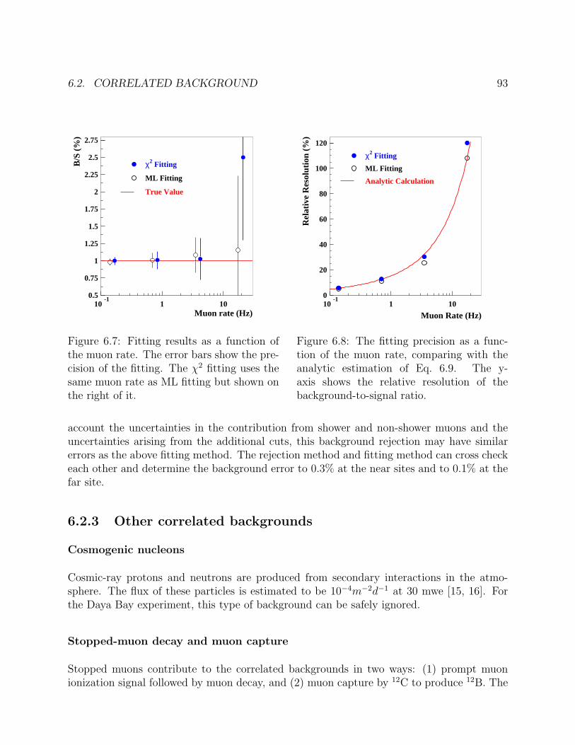
6.2. CORRELATED BACKGROUND 93
0.5
0.75
1
1.25
1.5
1.75
2
2.25
2.5
2.75
10-1
1 10
χ2 Fitting
ML Fitting
True Value
Muon rate (Hz)
B/S
(%
)
Figure 6.7: Fitting results as a function ofthe muon rate. The error bars show the pre-cision of the fitting. The χ2 fitting uses thesame muon rate as ML fitting but shown onthe right of it.
0
20
40
60
80
100
120
10-1
1 10
χ2 Fitting
ML Fitting
Analytic Calculation
Muon Rate (Hz)R
elat
ive
Res
olut
ion
(%)
Figure 6.8: The fitting precision as a func-tion of the muon rate, comparing with theanalytic estimation of Eq. 6.9. The y-axis shows the relative resolution of thebackground-to-signal ratio.
account the uncertainties in the contribution from shower and non-shower muons and theuncertainties arising from the additional cuts, this background rejection may have similarerrors as the above fitting method. The rejection method and fitting method can cross checkeach other and determine the background error to 0.3% at the near sites and to 0.1% at thefar site.
6.2.3 Other correlated backgrounds
Cosmogenic nucleons
Cosmic-ray protons and neutrons are produced from secondary interactions in the atmo-sphere. The flux of these particles is estimated to be 10−4m−2d−1 at 30 mwe [15, 16]. Forthe Daya Bay experiment, this type of background can be safely ignored.
Stopped-muon decay and muon capture
Stopped muons contribute to the correlated backgrounds in two ways: (1) prompt muonionization signal followed by muon decay, and (2) muon capture by 12C to produce 12B. The
94 CHAPTER 6. DETECTOR OVERBURDEN AND BACKGROUNDS
rate of untagged muons that decay in the detector is given by:
R = (1− ε)RµfdecayfE exp(−tv/τ), (6.10)
where Rµ is the muon rate, ε is the efficiency of the muon veto, fdecay is the fraction ofmuons that stopped and decayed, fE is the fraction of the decay electrons in the range ofthe neutron-capture energy (10%), τ is the muon lifetime and tv is the time window of theveto after any event. With a veto efficiency of 99.5% and 200 mwe of overburden, muondecay will contribute 0.3 events per day for the near detector. For the far detector the rateis reduced to <0.001 events per day. In cosmic rays 44% are muons, and 7.9% of them willbe captured by 12C. About 80% of the capture will end up in unstable states that typicallyresult in neutron emission. The background due to muon capture is smaller than that frommuon decay. While it is a non-trivial background for a detector with shallow overburden,backgrounds coming from stopped-muon decay and muon capture can be safely ignored inthe Daya Bay experiment.
6.3 Uncorrelated background
Natural radioactivity and slow neutrons induced by cosmic muons may occur within a giventime window accidentally to form an uncorrelated background. The coincidence rate is givenby
R = RγRnτ, (6.11)
where Rγ is the rate of natural radiation, Rn is the rate of spallation neutron, and τ is thelength of the time window. Since the geological environment and rock composition are verysimilar between Hong Kong and Daya Bay, the natural radioactivity in the Daya Bay sitescan be studied in Hong Kong. The group at Hong Kong University operates an undergroundlab in the Aberdeen Tunnel in Hong Kong. The spectrum of the natural radioactivity of therocks surrounding the lab is shown in Fig. 6.9.
Past experiments suppressed uncorrelated backgrounds with a combination of using care-fully selected construction materials, self-shielding, and using absorbers that have large neu-tron capture cross section. However, attention still needs to be paid to lower the detectorenergy threshold to under 1 MeV, the minimum visible energy of positron annihilation. Ahigher threshold will introduce a systematic error in the efficiency of detecting the positron,which is 0.8% in Chooz. Uncorrelated background can be measured by swapping detec-
tors [17]. The precision will be√
B/S. To achieve a background-to-signal ratio of 0.1%, therate of natural radioactivity above the 1 MeV threshold should be smaller than 50 Hz.
Radioactive background can come from a variety of sources:
• U/Th/K in the PMT glass.
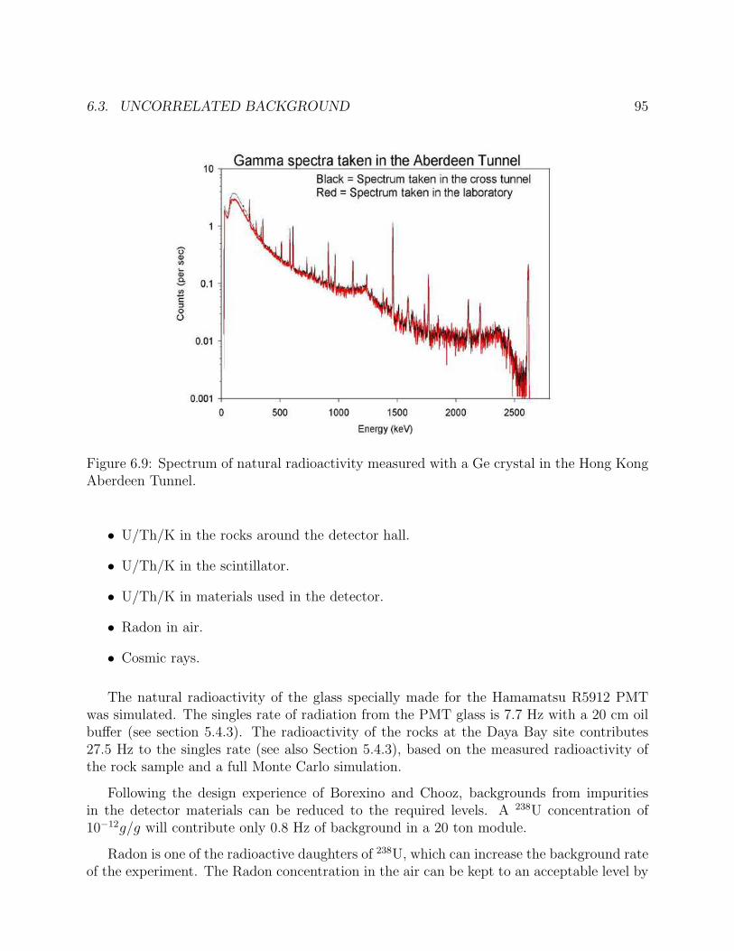
6.3. UNCORRELATED BACKGROUND 95
Figure 6.9: Spectrum of natural radioactivity measured with a Ge crystal in the Hong KongAberdeen Tunnel.
• U/Th/K in the rocks around the detector hall.
• U/Th/K in the scintillator.
• U/Th/K in materials used in the detector.
• Radon in air.
• Cosmic rays.
The natural radioactivity of the glass specially made for the Hamamatsu R5912 PMTwas simulated. The singles rate of radiation from the PMT glass is 7.7 Hz with a 20 cm oilbuffer (see section 5.4.3). The radioactivity of the rocks at the Daya Bay site contributes27.5 Hz to the singles rate (see also Section 5.4.3), based on the measured radioactivity ofthe rock sample and a full Monte Carlo simulation.
Following the design experience of Borexino and Chooz, backgrounds from impuritiesin the detector materials can be reduced to the required levels. A 238U concentration of10−12g/g will contribute only 0.8 Hz of background in a 20 ton module.
Radon is one of the radioactive daughters of 238U, which can increase the background rateof the experiment. The Radon concentration in the air can be kept to an acceptable level by

96 CHAPTER 6. DETECTOR OVERBURDEN AND BACKGROUNDS
ventilation. Since the neutrino detector modules are immersed in 2-meter thick water buffer,it is expected that the radon contribution can be safely ignored for Daya Bay.
The β decay of long lived radioactive isotopes produced by cosmic muons in the scin-tillator will contribute a couple of Hz at the near detector, and less than 0.1 Hz at the fardetector. The rate of accidental coincidence induced by muon decay or muon capture is lessthan the muon rate. So they can be ignored too.
6.4 Summary of backgrounds
Assuming a 99.5% muon veto efficiency, the three major backgrounds are summarized belowwhile the other sources are negligible. In our sensitivity study, the errors were taken as 100%for the accidental and fast neutron backgrounds. The isotope background can be measuredto an uncertainty of 0.3% and 0.1% at the near and far sites, respectively.
near site far site
Neutrino rate (/day) 560 80Natural radiation (Hz) <50 <50Single neutron (/day) 34 3
Accidental/Signal <0.05% <0.05%Fast neutron/Signal 0.14% 0.08%
8He9Li/Signal 0.5% 0.2%
Table 6.3: Summary of backgrounds.
The energy spectra of backgrounds are shown in Fig. 6.4. The background-to-signal ratiosare taken at the far site. The oscillation signal is the difference of the expected neutrinosignal without oscillation and the ”observed” signal with oscillation if sin2 2θ13 = 0.01.
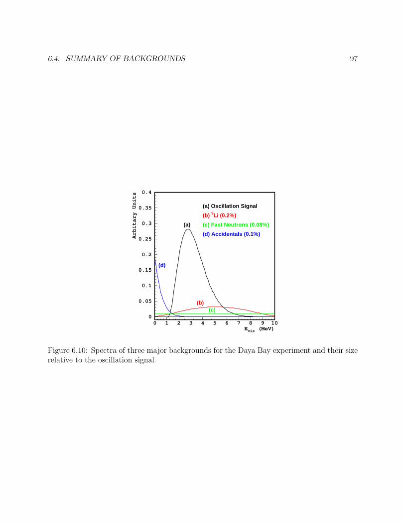
6.4. SUMMARY OF BACKGROUNDS 97
0
0.05
0.1
0.15
0.2
0.25
0.3
0.35
0.4
0 1 2 3 4 5 6 7 8 9 10Evis (MeV)
Arbitary Units
(b)
(b) 9Li (0.2%)
(c)
(c) Fast Neutrons (0.08%)
(d)
(d) Accidentals (0.1%)
(a)
(a) Oscillation Signal
Figure 6.10: Spectra of three major backgrounds for the Daya Bay experiment and their sizerelative to the oscillation signal.
Bibliography
[1] P. Antonioli et al., Astro. Phys. 7, 357 (1997).
[2] T. Gaisser, Cosmic Rays and Particle Physics, Cambridge University Press, 1991.
[3] Y. Muraki et al., Phys. Rev. D 28, 40 (1983).
[4] J. Kremer et al., Phys. Rev. Lett. 83, 4241 (1999)
[5] H. Jokisch et al., Phys. Rev. D 19, 1368 (1979).
[6] Y. F. Wang et al., Phys. Rev. D 64, 013012 (2001).
[7] M. Apollonio et al., Phys. Lett. 420B, 397 (1998); Phys. Lett. 466B, 415 (1999);Euro. Phys. J. C 27, 331 (2003).
[8] M. Ambrosio et al., (The MACRO Collaboration) Phys. Rev. D 52, 3793 (1995);M. Aglietta et al., (LVD Collaboration) Phys. Rev. D 60, 112001 (1999); Ch. Berger etal., (Frejus Collaboration) Phys. Rev. D 40, 2163 (1989).
[9] Atomic Data and Nuclear Data Tables, Vol. 78, No. 2 (July, 2001).
[10] T. Hagner et al., Astro. Phys. 14, 33 (2000).
[11] T. Araki et al., (KamLAND Collaboration) Phys. Rev. Lett. 94, 081801 (2005).
[12] K. S. McKinny, A Search for Astrophysical Electron Anti-neutrinos at KamLAND.Ph. D thesis, University of Alabama.
[13] Double Chooz LOI: hep-ex/0405032.
[14] John A. Rice, Mathematical Statistics and Data Analysis, second edition, WadsworthPublishing Co., Inc., 1993.
[15] F. Ashton, H. J. Edwards, and G. N. Kelly, J. Phys. A 4, 352 (1971).
[16] White paper report on using nuclear reactors to search for a value of θ13, hep-ex/0402041.
98

BIBLIOGRAPHY 99
[17] Y. F. Wang et al., Phys. Rev. D 62, 013012.
[18] A. Piepke et al., Nucl. Instr. and Meth. 432A, 392 (1999); F. Boehm et al., Phys. Rev. D62, 072002 (2000).

100 BIBLIOGRAPHY
Chapter 7
Systematic Issues
7.1 Overview
The control of systematic errors is critical to achieving the sin2 2θ13 sensitivity goal of thisexperiment. The most relevant previous experience is the Chooz experiment [1] which ob-tained sin2 2θ13 < 0.17 for ∆m2
31 = 2.5× 10⁻³eV2, the best limit to date, with a systematicuncertainty of 2.7% and statistical uncertainty of 2.8%. In order to achieve a sin2 2θ13 sen-sitivity below 0.01, both the statistical and systematic uncertainties have to be an order ofmagnitude smaller. The projected statistical error of the Daya Bay far detector is 0.2% withthree years data taking. In this section we discuss our strategy for achieving the level of sys-tematic error comparable to that of the statistical error. Achieving this very ambitious goalwill require extreme care and substantial effort that can only be realized by incorporatingrigid constraints in the design of the experiment.
There are three main sources of systematic uncertainties: reactor, background, and de-tector. Each source of error can be further classified into correlated and uncorrelated errors.
For the Chooz experiment, the systematic errors were due mostly to reactor uncertain-ties (2%), detector efficiency (1.5%), and the normalization of detector response which isdominated by the uncertainty in the number of free protons calculated from the hydrogen-to-carbon (H/C) ratio of the liquid scintillator (0.8%). The systematic uncertainties for theChooz experiment are presented in Table 7.2 for comparison. We will use them as referencefor estimating the effects of various improvements in detector technique and design.
Palo Verde [2] had systematic uncertainties similar to Chooz in detection efficiency andneutrino flux calculation. Palo Verde had additional errors related to background variations(the overburden was much less for Palo Verde) and trigger efficiency (due to the higherenergy threshold).
In KamLAND [3], uncertainties related to the reactors and fluxes are similar but a bit
101
102 CHAPTER 7. SYSTEMATIC ISSUES
larger than those of Chooz and Palo Verde. Other major sources of uncertainty for Kam-LAND include the total mass of liquid scintillator (2.1%), the fraction of liquid scintillatorwithin the fiducial volume (3.5%), and the level of background (1.8%). The KamLANDdetector systematic errors are listed in Table 7.2 as well.
The reduction in the systematic errors for Daya Bay relative to those of the Chooz exper-iment requires special detector techniques and design features. The primary considerationsthat led to the improved performance are listed below.
• The use of identical detectors at the near and far sites, a technique first proposed byMikaelyan et al. for the Kr2Det experiment in 1999 [4]. The event rate in the neardetector will be used to normalize the yield in the far detector. In this approach, allcorrelated errors essentially cancel in the ratio of the near and far signal rates. Un-correlated errors related to reactors can also be reduced to negligible level by carefullychoosing the locations of the near and far sites.
• Employ detector modules with three coaxial regions to reduce detector-related errorsby lowering the trigger threshold. The target volume is physically well defined by acentral region of Gd-loaded scintillator, surrounded by an intermediate region filledwith normal scintillator to catch the gammas leaking out of the central region. In thisdesign, no position cut is needed to determine the target volume, and the remainingerrors are dominated by the physical properties of the scintillator in the central volume.The third outer-most oil buffer region surrounding the gamma catcher separates thePMTs from the scintillator, reducing natural radioactivity background from the PMTs.Thus, the energy threshold of the detectors can be lowered to < 1.0 MeV, producingessentially 100% detection efficiency for the prompt positron.
• Detector components will be measured in advance of assembly, and divided among de-tector modules to equalize the properties of the modules. Differences will be distributedamong modules between the near and far sites to help cancel residual errors.
• Ensure sufficient overburden and shielding at all detector sites to reduce cosmic muoninduced backgrounds to a manageable level so they can be measured and subtractedout reliably.
• The use of multiple identical modules in each site enables the demonstration of sys-tematic error control at the limit of statistics.
• The detector modules are movable such that swapping of modules between the nearand far sites will cancel all detector related errors that remain unchanged before andafter swapping. The residual error is caused by the energy scale uncertainties, as wellas other site dependent errors.
With these improvements, the total detector-related systematic error is expected to be ∼0.2% per detector site which is comparable to the statistical uncertainty of ∼ 0.2% at the far
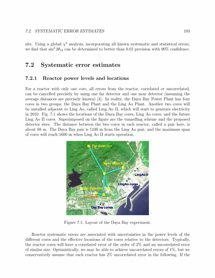
7.2. SYSTEMATIC ERROR ESTIMATES 103
site. Using a global χ2 analysis, incorporating all known systematic and statistical errors,we find that sin2 2θ13 can be determined to better than 0.01 precision with 90% confidence.
7.2 Systematic error estimates
7.2.1 Reactor power levels and locations
For a reactor with only one core, all errors from the reactor, correlated or uncorrelated,can be cancelled precisely by using one far detector and one near detector (assuming theaverage distances are precisely known) [4]. In reality, the Daya Bay Power Plant has fourcores in two groups, the Daya Bay Plant and the Ling Ao Plant. Another two cores willbe installed adjacent to Ling Ao, called Ling Ao II, which will start to generate electricityin 2010. Fig. 7.1 shows the locations of the Daya Bay cores, Ling Ao cores, and the futureLing Ao II cores. Superimposed on the figure are the tunnelling scheme and the proposeddetector sites. The distance between the two cores in each reactor, called a pair here, isabout 88 m. The Daya Bay pair is 1100 m from the Ling Ao pair, and the maximum spanof cores will reach 1600 m when Ling Ao II starts operation.
Figure 7.1: Layout of the Daya Bay experiment.
Reactor systematic errors are associated with uncertainties in the power levels of thedifferent cores and the effective locations of the cores relative to the detectors. Typically,the reactor cores will have a correlated error of the order of 2% and an uncorrelated errorof similar size. Optimistically, we may be able to achieve uncorrelated errors of 1%, but weconservatively assume that each reactor has 2% uncorrelated error in the following. If the
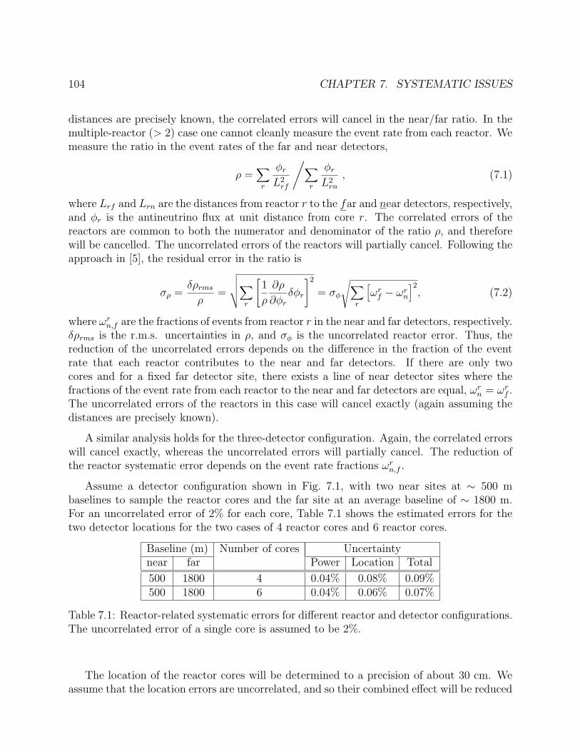
104 CHAPTER 7. SYSTEMATIC ISSUES
distances are precisely known, the correlated errors will cancel in the near/far ratio. In themultiple-reactor (> 2) case one cannot cleanly measure the event rate from each reactor. Wemeasure the ratio in the event rates of the far and near detectors,
ρ =∑r
φr
L2rf
/∑r
φr
L2rn
, (7.1)
where Lrf and Lrn are the distances from reactor r to the far and near detectors, respectively,and φr is the antineutrino flux at unit distance from core r. The correlated errors of thereactors are common to both the numerator and denominator of the ratio ρ, and thereforewill be cancelled. The uncorrelated errors of the reactors will partially cancel. Following theapproach in [5], the residual error in the ratio is
σρ =δρrms
ρ=
√√√√∑r
[1
ρ
∂ρ
∂φr
δφr
]2
= σφ
√∑r
[ωr
f − ωrn
]2, (7.2)
where ωrn,f are the fractions of events from reactor r in the near and far detectors, respectively.
δρrms is the r.m.s. uncertainties in ρ, and σφ is the uncorrelated reactor error. Thus, thereduction of the uncorrelated errors depends on the difference in the fraction of the eventrate that each reactor contributes to the near and far detectors. If there are only twocores and for a fixed far detector site, there exists a line of near detector sites where thefractions of the event rate from each reactor to the near and far detectors are equal, ωr
n = ωrf .
The uncorrelated errors of the reactors in this case will cancel exactly (again assuming thedistances are precisely known).
A similar analysis holds for the three-detector configuration. Again, the correlated errorswill cancel exactly, whereas the uncorrelated errors will partially cancel. The reduction ofthe reactor systematic error depends on the event rate fractions ωr
n,f .
Assume a detector configuration shown in Fig. 7.1, with two near sites at ∼ 500 mbaselines to sample the reactor cores and the far site at an average baseline of ∼ 1800 m.For an uncorrelated error of 2% for each core, Table 7.1 shows the estimated errors for thetwo detector locations for the two cases of 4 reactor cores and 6 reactor cores.
Baseline (m) Number of cores Uncertaintynear far Power Location Total
500 1800 4 0.04% 0.08% 0.09%500 1800 6 0.04% 0.06% 0.07%
Table 7.1: Reactor-related systematic errors for different reactor and detector configurations.The uncorrelated error of a single core is assumed to be 2%.
The location of the reactor cores will be determined to a precision of about 30 cm. Weassume that the location errors are uncorrelated, and so their combined effect will be reduced
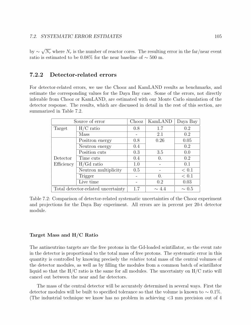
7.2. SYSTEMATIC ERROR ESTIMATES 105
by ∼ √Nr where Nr is the number of reactor cores. The resulting error in the far/near event
ratio is estimated to be 0.08% for the near baseline of ∼ 500 m.
7.2.2 Detector-related errors
For detector-related errors, we use the Chooz and KamLAND results as benchmarks, andestimate the corresponding values for the Daya Bay case. Some of the errors, not directlyinferable from Chooz or KamLAND, are estimated with our Monte Carlo simulation of thedetector response. The results, which are discussed in detail in the rest of this section, aresummarized in Table 7.2.
Source of error Chooz KamLAND Daya Bay
Target H/C ratio 0.8 1.7 0.2Mass - 2.1 0.2Positron energy 0.8 0.26 0.05Neutron energy 0.4 0.2Position cuts 0.3 3.5 0.0
Detector Time cuts 0.4 0. 0.2Efficiency H/Gd ratio 1.0 - 0.1
Neutron multiplicity 0.5 - < 0.1Trigger - 0. < 0.1Live time - 0.2 0.03
Total detector-related uncertainty 1.7 ∼ 4.4 ∼ 0.5
Table 7.2: Comparison of detector-related systematic uncertainties of the Chooz experimentand projections for the Daya Bay experiment. All errors are in percent per 20-t detectormodule.
Target Mass and H/C Ratio
The antineutrino targets are the free protons in the Gd-loaded scintillator, so the event ratein the detector is proportional to the total mass of free protons. The systematic error in thisquantity is controlled by knowing precisely the relative total mass of the central volumes ofthe detector modules, as well as by filling the modules from a common batch of scintillatorliquid so that the H/C ratio is the same for all modules. The uncertainty on H/C ratio willcancel out between the near and far detectors.
The mass of the central detector will be accurately determined in several ways. First thedetector modules will be built to specified tolerance so that the volume is known to ∼ 0.1%.(The industrial technique we know has no problem in achieving <3 mm precision out of 4
106 CHAPTER 7. SYSTEMATIC ISSUES
- 5 meters. We will make measurements of these volumes after construction to characterizethem to a precision better than 0.1%. We plan to fill each module from a common stainlesssteel tank maintained at constant temperature. We will measure the fluid volume usingpremium grade precision flowmeters with a repeatability of 0.02%. Several flowmeters willbe connected in series for redundancy. Residual topping off of the detector module to aspecified level (only about 20 kg since the volume is known and measured) is measured withthe flowmeters as well. We conservatively assign an error of 0.2% on the target mass basedon the absolute calibration of the flowmeters.
The absolute H/C ratio in Chooz was determined by using scintillator combustion andanalysis to 0.8% precision based on results from several laboratories. We will only requirethat the relative measurement on different samples be known, so an improved precision of0.2% or better is expected.
Energy Cut Efficiency
To reject uncorrelated backgrounds, Chooz employed a positron energy threshold of 1.3 MeV.This cut resulted in an estimated error of 0.8%, largely due to the trigger threshold changebecause of the degradation of liquid scintillator. The three-zone design of the Daya Baydetector and shielding makes it possible to lower this threshold to below 1 MeV while keepinguncorrelated backgrounds as low as 0.1%. The theoretical threshold of the visible energy ofthe neutrino events is 1.022 MeV, the annihilation energy of a positron at threshold with anelectron at rest. Due to finite energy resolution, the reconstructed energy will have a tailbelow 1 MeV. The systematic error associated with the inefficiency of this cut was studied byMonte Carlo simulation. The tail of the simulated energy spectrum is shown in Fig. 7.2 withthe full spectrum shown in the inset. For this simulation, 200 PMTs are used to measurethe energy deposited in a 20-ton module. The energy resolution is ∼ 15% at 1 MeV. Theinefficiencies are 0.32%, 0.37%, and 0.43% for cuts at 0.98 MeV, 1.0 MeV, and 1.02 MeV,respectively. Assuming the energy scale error is 2% at 1 MeV, this inefficiency variationwill produce a 0.05% error in the detected antineutrino rate. We have assumed that theGd-doped liquid scintillator has no dramatic degradation as Chooz suffered. A Palo Verdetype liquid scintillator will suffice for this requirement.
Another more important related issue is the neutron detection efficiency associated withthe capture of neutrons on Gd in the central detector volume. The capture releases severalgammas with 8 MeV total energy. Some gammas may escape from the active volume ofthe detector, resulting in a long tail in visible energy, as shown in Fig. 7.3. An energythreshold of about 6 MeV will be employed to cleanly select these delayed events. Whilegamma energy of natural radioactivity has an upper limit of ∼ 3.5 MeV, the radioactivityin liquid scintillator and acrylic vessel has contributions from gamma and beta particlessimultaneously. Especially 232Th contamination in gadolinium will contribute to the 4 - 6MeV energy region. Fig. 7.4 shows the data sample of Chooz before energy cut, in which
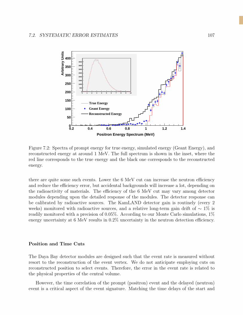
7.2. SYSTEMATIC ERROR ESTIMATES 107
0.2 0.4 0.6 0.8 1 1.2 1.4
Arb
itra
ry U
nit
s
0
50
100
150
200
250
300
350
400
True Energy
Geant Energy
Reconstructed Energy
0 1 2 3 4 5 6 7 8 9 100
500
1000
1500
2000
2500
3000
3500
4000
Positron Energy Spectrum (MeV)
option e1p
Figure 7.2: Spectra of prompt energy for true energy, simulated energy (Geant Energy), andreconstructed energy at around 1 MeV. The full spectrum is shown in the inset, where thered line corresponds to the true energy and the black one corresponds to the reconstructedenergy.
there are quite some such events. Lower the 6 MeV cut can increase the neutron efficiencyand reduce the efficiency error, but accidental backgrounds will increase a lot, depending onthe radioactivity of materials. The efficiency of the 6 MeV cut may vary among detectormodules depending upon the detailed response of the modules. The detector response canbe calibrated by radioactive sources. The KamLAND detector gain is routinely (every 2weeks) monitored with radioactive sources, and a relative long-term gain drift of ∼ 1% isreadily monitored with a precision of 0.05%. According to our Monte Carlo simulations, 1%energy uncertainty at 6 MeV results in 0.2% uncertainty in the neutron detection efficiency.
Position and Time Cuts
The Daya Bay detector modules are designed such that the event rate is measured withoutresort to the reconstruction of the event vertex. We do not anticipate employing cuts onreconstructed position to select events. Therefore, the error in the event rate is related tothe physical properties of the central volume.
However, the time correlation of the prompt (positron) event and the delayed (neutron)event is a critical aspect of the event signature. Matching the time delays of the start and
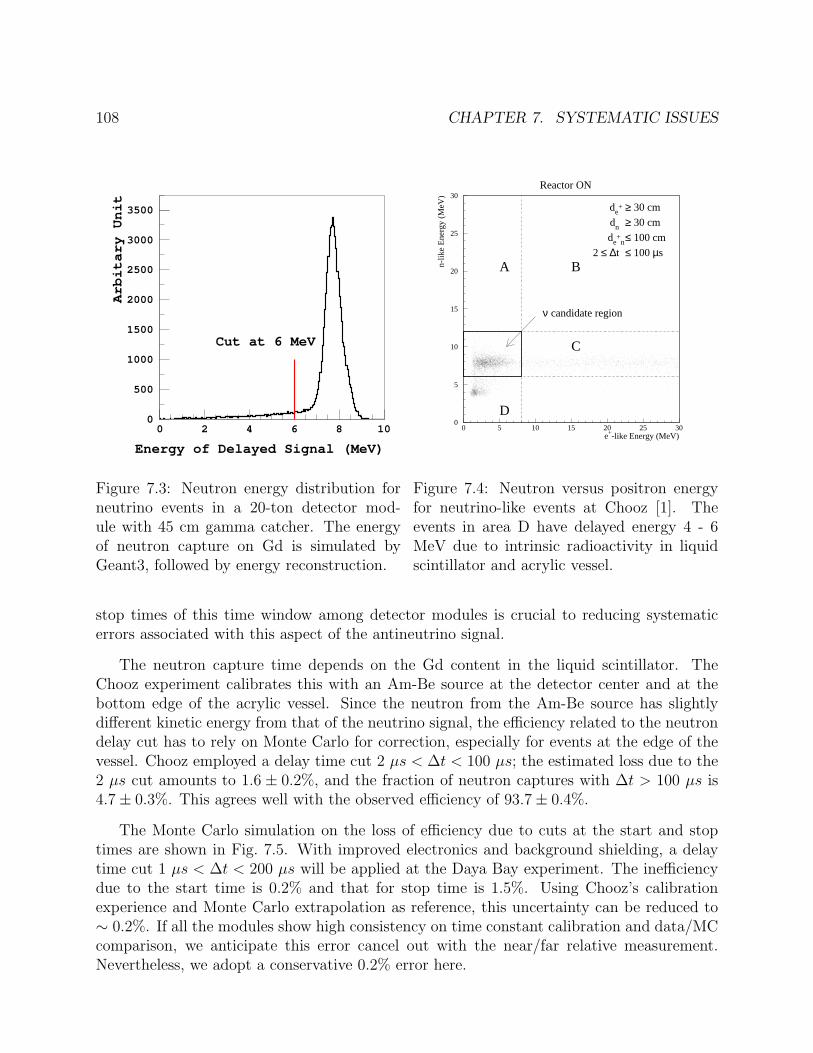
108 CHAPTER 7. SYSTEMATIC ISSUES
0
500
1000
1500
2000
2500
3000
3500
0 2 4 6 8 10
Energy of Delayed Signal (MeV)
Arbitary Unit
Cut at 6 MeV
Figure 7.3: Neutron energy distribution forneutrino events in a 20-ton detector mod-ule with 45 cm gamma catcher. The energyof neutron capture on Gd is simulated byGeant3, followed by energy reconstruction.
Reactor ON
0
5
10
15
20
25
30
0 5 10 15 20 25 30e+-like Energy (MeV)
n-lik
e E
nerg
y (M
eV)
A B
C
D
ν candidate region
de+
dn
de+
n
∆t
≥ 30 cm
≥ 30 cm
≤ 100 cm
≤ 100 µs2 ≤
Figure 7.4: Neutron versus positron energyfor neutrino-like events at Chooz [1]. Theevents in area D have delayed energy 4 - 6MeV due to intrinsic radioactivity in liquidscintillator and acrylic vessel.
stop times of this time window among detector modules is crucial to reducing systematicerrors associated with this aspect of the antineutrino signal.
The neutron capture time depends on the Gd content in the liquid scintillator. TheChooz experiment calibrates this with an Am-Be source at the detector center and at thebottom edge of the acrylic vessel. Since the neutron from the Am-Be source has slightlydifferent kinetic energy from that of the neutrino signal, the efficiency related to the neutrondelay cut has to rely on Monte Carlo for correction, especially for events at the edge of thevessel. Chooz employed a delay time cut 2 µs < ∆t < 100 µs; the estimated loss due to the2 µs cut amounts to 1.6 ± 0.2%, and the fraction of neutron captures with ∆t > 100 µs is4.7± 0.3%. This agrees well with the observed efficiency of 93.7± 0.4%.
The Monte Carlo simulation on the loss of efficiency due to cuts at the start and stoptimes are shown in Fig. 7.5. With improved electronics and background shielding, a delaytime cut 1 µs < ∆t < 200 µs will be applied at the Daya Bay experiment. The inefficiencydue to the start time is 0.2% and that for stop time is 1.5%. Using Chooz’s calibrationexperience and Monte Carlo extrapolation as reference, this uncertainty can be reduced to∼ 0.2%. If all the modules show high consistency on time constant calibration and data/MCcomparison, we anticipate this error cancel out with the near/far relative measurement.Nevertheless, we adopt a conservative 0.2% error here.
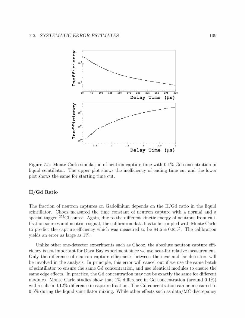
7.2. SYSTEMATIC ERROR ESTIMATES 109
10-2
10-1
50 75 100 125 150 175 200 225 250 275 300
Delay Time (µs)
Inefficiency
Delay Time (µs)
Inefficiency
10-4
10-3
10-2
0.5 1 1.5 2 2.5 3
Figure 7.5: Monte Carlo simulation of neutron capture time with 0.1% Gd concentration inliquid scintillator. The upper plot shows the inefficiency of ending time cut and the lowerplot shows the same for starting time cut.
H/Gd Ratio
The fraction of neutron captures on Gadolinium depends on the H/Gd ratio in the liquidscintillator. Chooz measured the time constant of neutron capture with a normal and aspecial tagged 252Cf source. Again, due to the different kinetic energy of neutrons from cali-bration sources and neutrino signal, the calibration data has to be coupled with Monte Carloto predict the capture efficiency which was measured to be 84.6 ± 0.85%. The calibrationyields an error as large as 1%.
Unlike other one-detector experiments such as Chooz, the absolute neutron capture effi-ciency is not important for Daya Bay experiment since we use near-far relative measurement.Only the difference of neutron capture efficiencies between the near and far detectors willbe involved in the analysis. In principle, this error will cancel out if we use the same batchof scintillator to ensure the same Gd concentration, and use identical modules to ensure thesame edge effects. In practice, the Gd concentration may not be exactly the same for differentmodules. Monte Carlo studies show that 1% difference in Gd concentration (around 0.1%)will result in 0.12% difference in capture fraction. The Gd concentration can be measured to0.5% during the liquid scintillator mixing. While other effects such as data/MC discrepancy
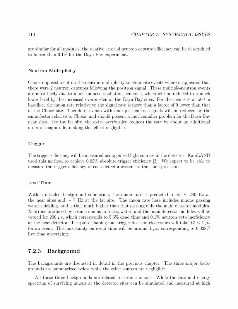
110 CHAPTER 7. SYSTEMATIC ISSUES
are similar for all modules, the relative error of neutron capture efficiency can be determinedto better than 0.1% for the Daya Bay experiment.
Neutron Multiplicity
Chooz imposed a cut on the neutron multiplicity to eliminate events where it appeared thatthere were 2 neutron captures following the positron signal. These multiple-neutron eventsare most likely due to muon-induced spallation neutrons, which will be reduced to a muchlower level by the increased overburden at the Daya Bay sites. For the near site at 500 mbaseline, the muon rate relative to the signal rate is more than a factor of 9 lower than thatof the Chooz site. Therefore, events with multiple neutron signals will be reduced by thesame factor relative to Chooz, and should present a much smaller problem for the Daya Baynear sites. For the far site, the extra overburden reduces the rate by about an additionalorder of magnitude, making this effect negligible.
Trigger
The trigger efficiency will be measured using pulsed light sources in the detector. KamLANDused this method to achieve 0.02% absolute trigger efficiency [3]. We expect to be able tomeasure the trigger efficiency of each detector system to the same precision.
Live Time
With a detailed background simulation, the muon rate is predicted to be ∼ 280 Hz atthe near sites and ∼ 7 Hz at the far site. The muon rate here includes muons passingwater shielding, and is thus much higher than that passing only the main detector modules.Neutrons produced by cosmic muons in rocks, water, and the main detector modules will bevetoed for 200 µs, which corresponds to 5.6% dead time and 0.1% neutron veto inefficiencyat the near detector. The pulse shaping and trigger decision electronics will take 0.5 ∼ 1 µsfor an event. The uncertainty on event time will be around 1 µs, corresponding to 0.028%live time uncertainty.
7.2.3 Background
The backgrounds are discussed in detail in the previous chapter. The three major back-grounds are summarized below while the other sources are negligible.
All these three backgrounds are related to cosmic muons. While the rate and energyspectrum of surviving muons at the detector sites can be simulated and measured at high
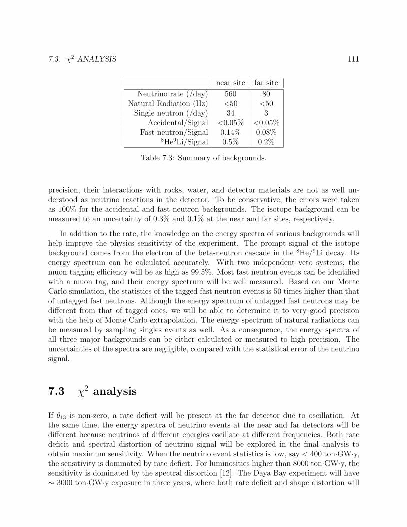
7.3. χ2 ANALYSIS 111
near site far site
Neutrino rate (/day) 560 80Natural Radiation (Hz) <50 <50
Single neutron (/day) 34 3Accidental/Signal <0.05% <0.05%
Fast neutron/Signal 0.14% 0.08%8He9Li/Signal 0.5% 0.2%
Table 7.3: Summary of backgrounds.
precision, their interactions with rocks, water, and detector materials are not as well un-derstood as neutrino reactions in the detector. To be conservative, the errors were takenas 100% for the accidental and fast neutron backgrounds. The isotope background can bemeasured to an uncertainty of 0.3% and 0.1% at the near and far sites, respectively.
In addition to the rate, the knowledge on the energy spectra of various backgrounds willhelp improve the physics sensitivity of the experiment. The prompt signal of the isotopebackground comes from the electron of the beta-neutron cascade in the 8He/9Li decay. Itsenergy spectrum can be calculated accurately. With two independent veto systems, themuon tagging efficiency will be as high as 99.5%. Most fast neutron events can be identifiedwith a muon tag, and their energy spectrum will be well measured. Based on our MonteCarlo simulation, the statistics of the tagged fast neutron events is 50 times higher than thatof untagged fast neutrons. Although the energy spectrum of untagged fast neutrons may bedifferent from that of tagged ones, we will be able to determine it to very good precisionwith the help of Monte Carlo extrapolation. The energy spectrum of natural radiations canbe measured by sampling singles events as well. As a consequence, the energy spectra ofall three major backgrounds can be either calculated or measured to high precision. Theuncertainties of the spectra are negligible, compared with the statistical error of the neutrinosignal.
7.3 χ2 analysis
If θ13 is non-zero, a rate deficit will be present at the far detector due to oscillation. Atthe same time, the energy spectra of neutrino events at the near and far detectors will bedifferent because neutrinos of different energies oscillate at different frequencies. Both ratedeficit and spectral distortion of neutrino signal will be explored in the final analysis toobtain maximum sensitivity. When the neutrino event statistics is low, say < 400 ton·GW·y,the sensitivity is dominated by rate deficit. For luminosities higher than 8000 ton·GW·y, thesensitivity is dominated by the spectral distortion [12]. The Daya Bay experiment will have∼ 3000 ton·GW·y exposure in three years, where both rate deficit and shape distortion will
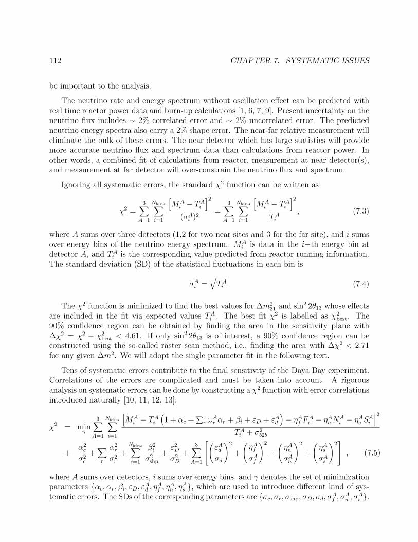
112 CHAPTER 7. SYSTEMATIC ISSUES
be important to the analysis.
The neutrino rate and energy spectrum without oscillation effect can be predicted withreal time reactor power data and burn-up calculations [1, 6, 7, 9]. Present uncertainty on theneutrino flux includes ∼ 2% correlated error and ∼ 2% uncorrelated error. The predictedneutrino energy spectra also carry a 2% shape error. The near-far relative measurement willeliminate the bulk of these errors. The near detector which has large statistics will providemore accurate neutrino flux and spectrum data than calculations from reactor power. Inother words, a combined fit of calculations from reactor, measurement at near detector(s),and measurement at far detector will over-constrain the neutrino flux and spectrum.
Ignoring all systematic errors, the standard χ2 function can be written as
χ2 =3∑
A=1
Nbins∑
i=1
[MA
i − TAi
]2
(σAi )2
=3∑
A=1
Nbins∑
i=1
[MA
i − TAi
]2
TAi
, (7.3)
where A sums over three detectors (1,2 for two near sites and 3 for the far site), and i sumsover energy bins of the neutrino energy spectrum. MA
i is data in the i−th energy bin atdetector A, and TA
i is the corresponding value predicted from reactor running information.The standard deviation (SD) of the statistical fluctuations in each bin is
σAi =
√TA
i . (7.4)
The χ2 function is minimized to find the best values for ∆m231 and sin2 2θ13 whose effects
are included in the fit via expected values TAi . The best fit χ2 is labelled as χ2
best. The90% confidence region can be obtained by finding the area in the sensitivity plane with∆χ2 = χ2 − χ2
best < 4.61. If only sin2 2θ13 is of interest, a 90% confidence region can beconstructed using the so-called raster scan method, i.e., finding the area with ∆χ2 < 2.71for any given ∆m2. We will adopt the single parameter fit in the following text.
Tens of systematic errors contribute to the final sensitivity of the Daya Bay experiment.Correlations of the errors are complicated and must be taken into account. A rigorousanalysis on systematic errors can be done by constructing a χ2 function with error correlationsintroduced naturally [10, 11, 12, 13]:
χ2 = minγ
3∑
A=1
Nbins∑
i=1
[MA
i − TAi
(1 + αc +
∑r ωA
r αr + βi + εD + εAd
)− ηA
f FAi − ηA
n NAi − ηA
s SAi
]2
TAi + σ2
b2b
+α2
c
σ2c
+∑r
α2r
σ2r
+Nbins∑
i=1
β2i
σ2shp
+ε2
D
σ2D
+3∑
A=1
(εA
d
σd
)2
+
(ηA
f
σAf
)2
+
(ηA
n
σAn
)2
+
(ηA
s
σAs
)2 , (7.5)
where A sums over detectors, i sums over energy bins, and γ denotes the set of minimizationparameters {αc, αr, βi, εD, εA
d , ηAf , ηA
n , ηAs }, which are used to introduce different kind of sys-
tematic errors. The SDs of the corresponding parameters are {σc, σr, σshp, σD, σd, σAf , σA
n , σAs }.
7.3. χ2 ANALYSIS 113
For each energy bin, there is a statistical error TAi and a bin-to-bin systematic error σb2b.
For each point in the oscillation space, the χ2 function has to be minimized with respect tothe parameters γ.
Assuming each error can be approximated by a Gaussian, this form of χ2 can be provento be strictly equivalent to the more familiar covariance matrix form χ2 = (M−T )T V −1(M−T ) [10], where V is the covariance matrix of (M−T ) with systematic errors included properly.The systematic errors are described one by one in the following.
Reactor-related correlated error: σc
Reactor-related correlated error accounts for normalization errors of the event rate commonto all reactor cores, such as energy released per fission and neutrino yield per fission. Withnear-far relative measurement, fully correlated error has almost no impact on the sensitivity.Nevertheless, we use σc = 2% in the sensitivity analysis.
Reactor-related uncorrelated error: σr
Reactor-related uncorrelated error is the normalization error of the event rate which variesindependently from core to core, such as reactor power and related burn-up calculation.It is discussed in section 7.2.1; this error does not exactly cancel out by near-far relativemeasurement for a complex core layout such as Daya Bay. We take the uncorrelated error ofa single core to be σr = 2% while we believe 1% could be reached. ωA
r is the event fractioncontribution from core r to detector A, with the constraint
∑r ωA
r = 1 for each detector.Error reduction will be automatically realized with the minimization of αr. For well chosensites, the residual error could be as low as 0.04% (see Table 7.1), and thus has very littleimpact. For poorly chosen sites or one near detector scenario, the residual error might havelarge impact.
Shape error: σshp
Shape error is the uncertainty on neutrino energy spectra calculated from reactor informa-tion, σshp ∼ 2%. This error is uncorrelated between different energy bins but correlatedbetween different detectors. Since we have enough statistics at near detector to measureneutrino energy spectrum to much better than 2%, in addition to this calculation, it haslittle impact for Daya Bay sensitivity.
114 CHAPTER 7. SYSTEMATIC ISSUES
Detector-related correlated error: σD
Some detection errors are common to all detectors, such as H/Gd ratio, H/C ratio, neutroncapture time on Gd, and edge effect, assuming we use the same batch of liquid scintillatorand identical detectors. Based on Chooz’s experience, σD is (1 - 2)%. Like other fullycorrelated errors, it has almost no impact on sensitivity.
Detector-related uncorrelated error: σd
Detector-related uncorrelated errors include the mass of active volume, live time, etc., whichdo cancel out with near-far measurement. It is described in section 7.2.2, and estimated tobe σd = 0.5% for a single detector module.
Background-related error: σAf , σA
n , and σAs
There are three kinds of major backgrounds in the Daya Bay experiment: Fast neutronsFA
i , isotopes SAi , and accidental backgrounds NA
i . As described above, their spectra can beeither calculated or measured to a very good precision, compared with the neutrino oscilla-tion signal. As a consequence, the bin-to-bin uncertainties due to background subtraction,which should be uncorrelated between energy bins and different sites, can be normally ig-nored. While we know the spectral shape of each individual background, the rate has a largeuncertainty. Our Monte Carlo simulation shows that the rate of fast neutrons FA =
∑i F
Ai
is 0.14% of the neutrino signal (TA =∑
i TAi ) at the near sites (A=1,2) and 0.08% of the
signal at the far site (A=3). The rate of isotopes SA =∑
i SAi is 0.5% of TA at the near
sites and 0.2% of TA at the far site. The rate of accidental backgrounds NA =∑
i NAi is
taken to be 0.05% of TA. To be conservative, we assume the estimation of the fast neutronand accidental backgrounds carry 100% uncertainty and the isotope backgrounds can bemeasured to a 60% precision at the near sites and to a 50% precision at the far site, i.e.,σA
f = σAn = 100%, σ1,2
s = 60%, σ3s = 50%.
Bin-to-bin error: σb2b
Bin-to-bin error is systematic error that is uncorrelated between energy bins and uncorrelatedbetween different detector modules. The bin-to-bin errors normally arise from the differentenergy scale at different energies and background subtraction. Up to now, the only reactorneutrino experiment that performed spectral analysis with large statistics is Bugey, whichhas bin-to-bin error of order of 0.5% [7, 8]. With better designed detector and much fewerbackground, we should have smaller bin-to-bin error than Bugey. The bin-to-bin error canbe studied by comparing the spectra of two detector modules at the same site. We will use0.5% in the sensitivity analysis.
7.4. SIDE-BY-SIDE CALIBRATION AND DETECTOR SWAPPING 115
Other errors:
The energy resolution of the detector is ∼ 14%/√
E(MeV), which is 5% at 8 MeV or 14% at1 MeV. Due to energy smearing, the spectra are distorted. However, the energy bins usedfor sensitivity analysis (∼ 30 bins) is 2 ∼ 6 times larger than the energy resolution, and thedistortion happens at all detectors in the same way, energy resolution has almost no impacton the final sensitivity.
Detector energy scale error has significant impact on detection errors (neutron efficiencyand positron efficiency). It is taken into account in σd. At the same time, an energy scaleerror will shift the whole spectrum, thus directly impacting the analysis, especially on thebest fit values. However, this shift is not a distortion, and cannot mimic oscillation. It hasvery little impact on sensitivity computations.
Current knowledge on θ12 and ∆m21 has around 10% errors. Although the net oscillationeffect at Daya Bay baseline is related to θ13 only, the subtraction of θ12 oscillation effectsmight bring errors.
We have studied the above three error sources and found none of them having visibleimpact on the sensitivity of the Daya Bay experiment. For simplicity, they are ignored inour χ2 analysis of sensitivity.
There may be other unexpected errors at the level of a few per mil since our experienceis only from measurements at the 3% level. For instance, neutrinos from spent fuel, duringor near by fuel recycle period, or other man-made neutrino sources such as nuclear-poweredsubmarines may affect our results. Unexpected efficiency variation could also occur at thelevel of 0.1%. Therefore redundancy is a must for such a precision experiment. This issuewill be discussed further in the next section.
7.4 Side-by-side calibration and detector swapping
The sensitivity of the Daya Bay experiment largely depends on detector uncorrelated error(relative detection efficiency error). With improved design, the detector systematic errorcould be lowered to ∼ 0.5%, based on Chooz’s experience. Nevertheless, it is a challenge tothe detector fabrication and operation. Furthermore, the detection error is a combination ofmany sources. Their correlations are not easy to work out. How to combine them may becontroversial. Side-by-side calibration of detectors can clarify this uncertainty.
If we put two detectors at the same site for the same period of time, the backgrounds andneutrino flux will be identical for them. The only difference is their detection efficiency. Nomatter what the origins of the systematic errors are, the detection efficiency can be correctedto the same level, up to the precision of statistics. For a 20-ton detector module at 360 maway from two 2.9 GW reactor cores (at Daya Bay near site), the statistical error is 0.3%
116 CHAPTER 7. SYSTEMATIC ISSUES
with 100 days’ data and 75% detection efficiency. The relative detection efficiency error couldthen be determined within
√2× 0.3% = 0.42% in 100 days. That will be a straightforward
check of detector systematics.
One advantage of the horizontal tunnel of the Daya Bay experiment is the ability to movethe detector modules conveniently. Swapping detectors between the near and far sites willeliminate detection efficiency errors and greatly improve the physics sensitivity. Suppose aflux deficit is observed at the far site, it may be attributed to neutrino oscillation, or it maybe due to lower detection efficiency at the far site compared with the near site. Then weswap the detectors at the near and far sites. If the deficit is due to detection efficiency, weshould observe a flux surplus at the far site, compared with the near detector which hasa lower detection efficiency. If the previously observed flux deficit is due to oscillation, weshould again observe deficit at far site. By swapping detectors, we have an over-constrainton detector uncorrelated errors in sensitivity analysis, which will essentially cancel out thisimportant systematic error.
To cancel the detector uncorrelated error, a detector module should have equal datafraction at the near and far sites. For example, if the data of a given module contributes1/4 of the total data volume taken at the Daya Bay near site, the data of the same moduleshould also contribute 1/4 of the whole data volume at the far site. If the data volumesare not equal, then part of the detector error cannot be cancelled out. For a pressurizedwater reactor, the average up-time is around 80% to 85%. The idle time is normally due toshutdown for refuelling and maintenance which takes 4∼6 weeks every 12 months. The twocores in a cluster will be shut down in turn. It is possible that one data taking period has ∼10% more data than another. Although the detector error cannot be cancelled out exactly,the residual error caused by different data volume will be an order of magnitude lower thanthat without swapping. The impact on sensitivity is much smaller.
A prerequisite for successful swapping is that the detection efficiency of a detector is keptunchanged before and after moving. One possible source of efficiency variation is the energyscale. To monitor liquid scintillator aging and other time dependent effects of detectors, theenergy calibration is performed from time to time. The energy scale is not necessarily thesame after moving. The precision of energy calibration can be as accurate as 0.5 to 1%. Thecorresponding neutron efficiency error will be 0.1 to 0.2% from our detector simulation. Sowe assume the residual detection efficiency error is 0.2% with swapping measurement.
Moving a detector of total weight of 100 tonnes for 2 km may cause unknown variations ofdetection efficiency. This could be fatal for such a precision experiment if we cannot discoverthe problem early and solve it. Side-by-side calibration enables us to get full control of thesystematics by monitoring detectors at the same site continuously. Variation of detectionefficiency after detector swapping can be identified up to the precision of statistics.
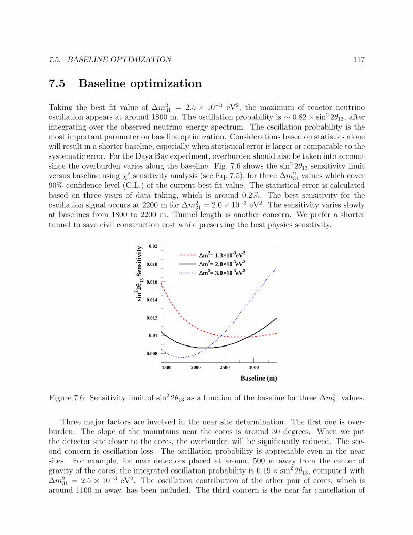
7.5. BASELINE OPTIMIZATION 117
7.5 Baseline optimization
Taking the best fit value of ∆m231 = 2.5 × 10⁻³ eV2, the maximum of reactor neutrino
oscillation appears at around 1800 m. The oscillation probability is ∼ 0.82× sin2 2θ13, afterintegrating over the observed neutrino energy spectrum. The oscillation probability is themost important parameter on baseline optimization. Considerations based on statistics alonewill result in a shorter baseline, especially when statistical error is larger or comparable to thesystematic error. For the Daya Bay experiment, overburden should also be taken into accountsince the overburden varies along the baseline. Fig. 7.6 shows the sin2 2θ13 sensitivity limitversus baseline using χ2 sensitivity analysis (see Eq. 7.5), for three ∆m2
31 values which cover90% confidence level (C.L.) of the current best fit value. The statistical error is calculatedbased on three years of data taking, which is around 0.2%. The best sensitivity for theoscillation signal occurs at 2200 m for ∆m2
31 = 2.0× 10⁻³ eV2. The sensitivity varies slowlyat baselines from 1800 to 2200 m. Tunnel length is another concern. We prefer a shortertunnel to save civil construction cost while preserving the best physics sensitivity.
0.008
0.01
0.012
0.014
0.016
0.018
0.02
1500 2000 2500 3000
∆m2= 1.3×10⁻³eV2
∆m2= 2.0×10⁻³eV2
∆m2= 3.0×10⁻³eV2
Baseline (m)
sin2 2θ
13 S
ensi
tivi
ty
Figure 7.6: Sensitivity limit of sin2 2θ13 as a function of the baseline for three ∆m231 values.
Three major factors are involved in the near site determination. The first one is over-burden. The slope of the mountains near the cores is around 30 degrees. When we putthe detector site closer to the cores, the overburden will be significantly reduced. The sec-ond concern is oscillation loss. The oscillation probability is appreciable even in the nearsites. For example, for near detectors placed at around 500 m away from the center ofgravity of the cores, the integrated oscillation probability is 0.19× sin2 2θ13, computed with∆m2
31 = 2.5 × 10⁻³ eV2. The oscillation contribution of the other pair of cores, which isaround 1100 m away, has been included. The third concern is the near-far cancellation of

118 CHAPTER 7. SYSTEMATIC ISSUES
reactor errors. As shown in the previous section, the cancellation is not exact if detectorsare too close to the reactor complex.
With a detailed topographic map of the Daya Bay site, the muon flux are simulatedwith a MUSIC-based program, as described in the last chapter. The simulation is performedwith a grid size of 50 m, as shown in Fig. 7.7, in the area that the optimal detector site maylocate. At each grid point, the flux and mean energy of the survived muons are obtained. Theisotope background can be directly calculated with the cross section extrapolated to the muonenergy. The fast neutron background and single neutrons, thus the accidental backgrounds,are simulated at several typical sites, using the algorithm described in last chapter. Then thebackgrounds are extrapolated to other sites using the power law, background ∝ E0.74
µ , sincethe neutron yield follows the same power law and the neutron energy spectrum depends onlyslightly on muon energy.
m400 500 600 700 800 900
m
2050
2100
2150
2200
2250
2300
2350
2400388
397
376
345
314
291
280
280
414
398
367
337
314
303
307
303
432
403
370
347
344
327
329
324
418
403
398
383
360
342
331
329
443
428
394
366
350
336
331
321
460
419
398
383
363
364
355
346
462
437
415
387
372
370
350
344
452
427
408
384
360
347
338
335
443
416
386
368
359
330
315
313
417
414
384
355
340
338
325
299
0.027 148
0.030 143
0.034 141
0.039 136
0.044 131
0.050 127
0.057 125
0.066 121
0.025 151
0.028 146
0.032 143
0.036 139
0.040 137
0.046 132
0.051 128
0.059 125
0.024 152
0.027 149
0.030 145
0.033 142
0.037 139
0.042 135
0.047 131
0.053 129
0.023 155
0.026 152
0.028 147
0.031 145
0.035 140
0.039 138
0.044 135
0.049 133
0.023 156
0.025 153
0.028 148
0.030 146
0.034 144
0.037 139
0.042 137
0.046 134
0.022 156
0.025 152
0.027 150
0.030 145
0.033 144
0.036 141
0.040 138
0.045 135
0.023 155
0.025 154
0.027 150
0.030 147
0.033 142
0.036 140
0.040 139
0.044 136
0.024 154
0.026 151
0.028 148
0.030 146
0.033 145
0.037 141
0.040 138
0.045 134
0.025 152
0.027 150
0.029 148
0.031 146
0.034 142
0.038 139
0.041 137
0.046 133
0.027 148
0.029 148
0.031 145
0.033 142
0.036 140
0.039 138
0.043 134
0.048 132
Figure 7.7: Muon flux in the vicinity of the far site. The blue lines shows the contour of themountain and the red dots are the grid points that the calculation is carried on.
Based on the background simulation at different possible sites, a global χ2 analysis iscarried on for each possible site configuration. Now the grid is finer at an interval of 10 m,by interpolate the background simulated as above. The inputs of the χ2 analysis has beendescribed in last section. The optimal near and far sites are chosen for the best sin2 2θ13
sensitivity. Fig. 7.8 shows the optimal sites in red triangles, as well as the sensitivity contourwhen one site varies and the other two are fixed at the optimal sites. The optimal sitesare off the perpendicular bisectors largely due to overburden. The average distances of theoptimal sites to three pairs of cores are listed in Table 7.4.
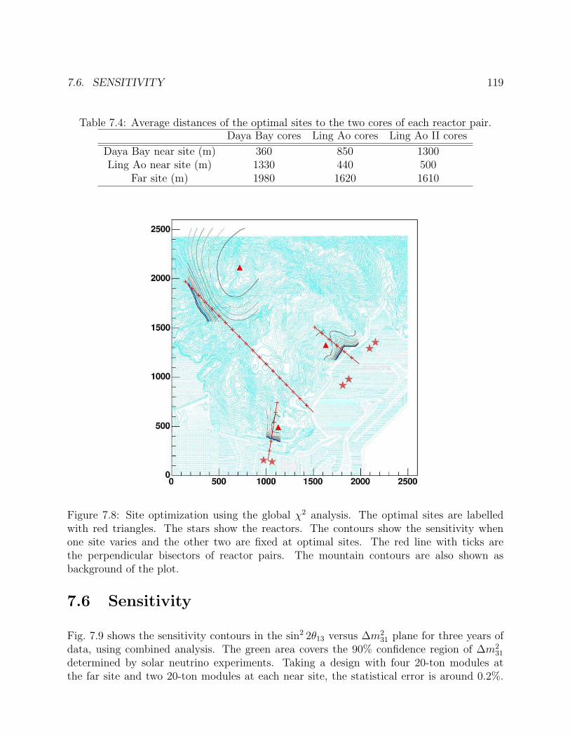
7.6. SENSITIVITY 119
Table 7.4: Average distances of the optimal sites to the two cores of each reactor pair.Daya Bay cores Ling Ao cores Ling Ao II cores
Daya Bay near site (m) 360 850 1300Ling Ao near site (m) 1330 440 500
Far site (m) 1980 1620 1610
Figure 7.8: Site optimization using the global χ2 analysis. The optimal sites are labelledwith red triangles. The stars show the reactors. The contours show the sensitivity whenone site varies and the other two are fixed at optimal sites. The red line with ticks arethe perpendicular bisectors of reactor pairs. The mountain contours are also shown asbackground of the plot.
7.6 Sensitivity
Fig. 7.9 shows the sensitivity contours in the sin2 2θ13 versus ∆m231 plane for three years of
data, using combined analysis. The green area covers the 90% confidence region of ∆m231
determined by solar neutrino experiments. Taking a design with four 20-ton modules atthe far site and two 20-ton modules at each near site, the statistical error is around 0.2%.
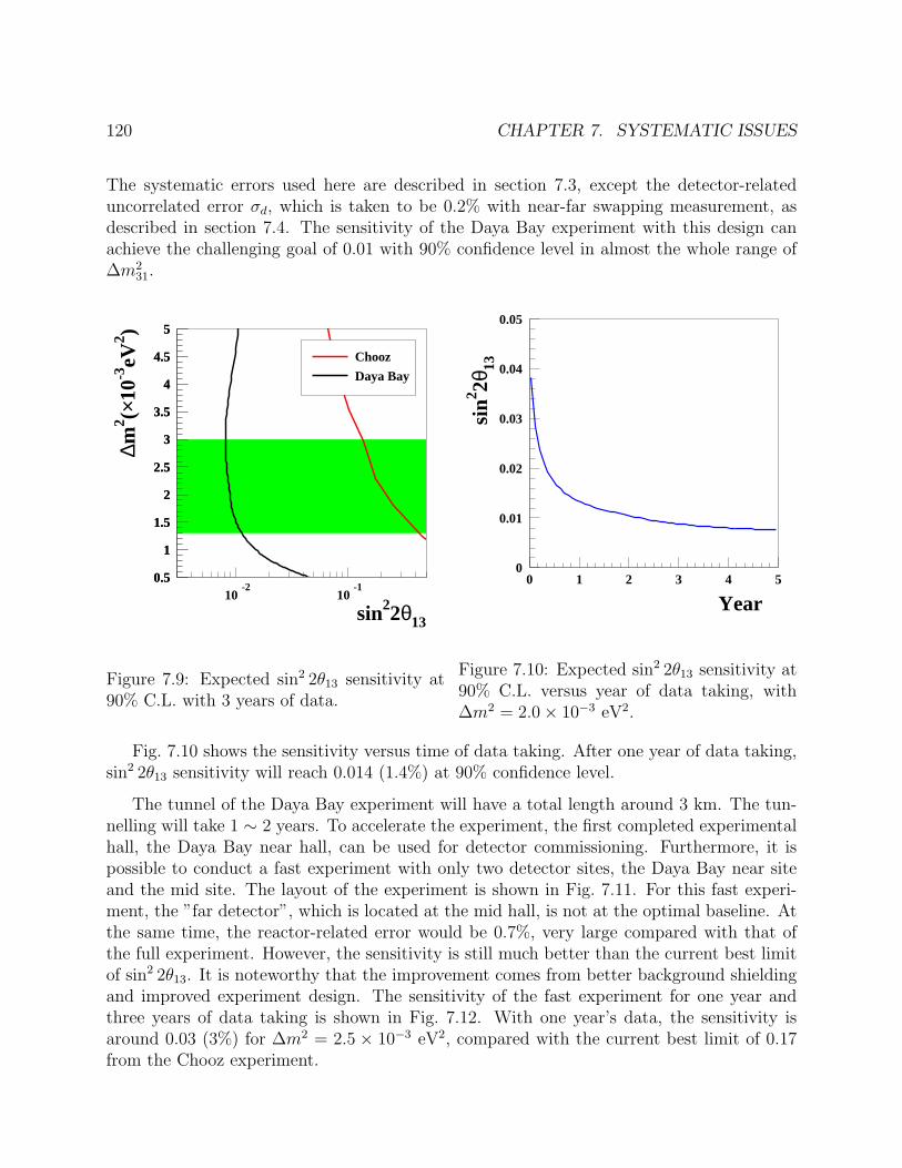
120 CHAPTER 7. SYSTEMATIC ISSUES
The systematic errors used here are described in section 7.3, except the detector-relateduncorrelated error σd, which is taken to be 0.2% with near-far swapping measurement, asdescribed in section 7.4. The sensitivity of the Daya Bay experiment with this design canachieve the challenging goal of 0.01 with 90% confidence level in almost the whole range of∆m2
31.
0.5
1
1.5
2
2.5
3
3.5
4
4.5
5
10-2
10-1
0.5
1
1.5
2
2.5
3
3.5
4
4.5
5
Chooz
Daya Bay
sin22θ13
∆m2 (×
10-3
eV2 )
Figure 7.9: Expected sin2 2θ13 sensitivity at90% C.L. with 3 years of data.
0
0.01
0.02
0.03
0.04
0.05
0 1 2 3 4 5
Year
sin2 2θ
13
Figure 7.10: Expected sin2 2θ13 sensitivity at90% C.L. versus year of data taking, with∆m2 = 2.0× 10⁻³ eV2.
Fig. 7.10 shows the sensitivity versus time of data taking. After one year of data taking,sin2 2θ13 sensitivity will reach 0.014 (1.4%) at 90% confidence level.
The tunnel of the Daya Bay experiment will have a total length around 3 km. The tun-nelling will take 1 ∼ 2 years. To accelerate the experiment, the first completed experimentalhall, the Daya Bay near hall, can be used for detector commissioning. Furthermore, it ispossible to conduct a fast experiment with only two detector sites, the Daya Bay near siteand the mid site. The layout of the experiment is shown in Fig. 7.11. For this fast experi-ment, the ”far detector”, which is located at the mid hall, is not at the optimal baseline. Atthe same time, the reactor-related error would be 0.7%, very large compared with that ofthe full experiment. However, the sensitivity is still much better than the current best limitof sin2 2θ13. It is noteworthy that the improvement comes from better background shieldingand improved experiment design. The sensitivity of the fast experiment for one year andthree years of data taking is shown in Fig. 7.12. With one year’s data, the sensitivity isaround 0.03 (3%) for ∆m2 = 2.5 × 10⁻³ eV2, compared with the current best limit of 0.17from the Chooz experiment.
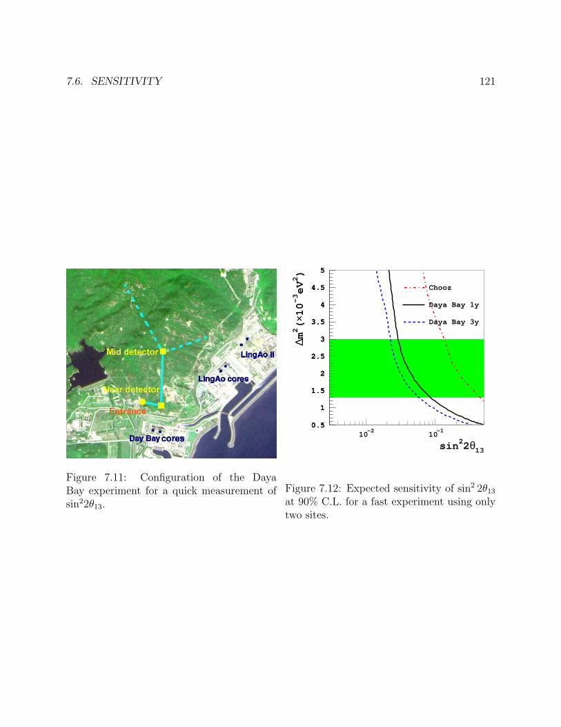
7.6. SENSITIVITY 121
Figure 7.11: Configuration of the DayaBay experiment for a quick measurement ofsin22θ13.
0.5
1
1.5
2
2.5
3
3.5
4
4.5
5
10-2
10-1
0.5
1
1.5
2
2.5
3
3.5
4
4.5
5
Chooz
Daya Bay 1y
Daya Bay 3y
sin22θ13
∆m2(
×10-3eV2)
Figure 7.12: Expected sensitivity of sin2 2θ13
at 90% C.L. for a fast experiment using onlytwo sites.
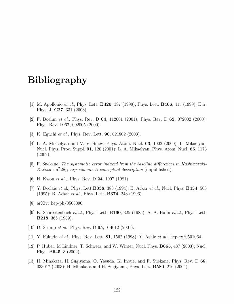
Bibliography
[1] M. Apollonio et al., Phys. Lett. B420, 397 (1998); Phys. Lett. B466, 415 (1999); Eur.Phys. J. C27, 331 (2003).
[2] F. Boehm et al., Phys. Rev. D 64, 112001 (2001); Phys. Rev. D 62, 072002 (2000);Phys. Rev. D 62, 092005 (2000).
[3] K. Eguchi et al., Phys. Rev. Lett. 90, 021802 (2003).
[4] L. A. Mikaelyan and V. V. Sinev, Phys. Atom. Nucl. 63, 1002 (2000); L. Mikaelyan,Nucl. Phys. Proc. Suppl. 91, 120 (2001); L. A. Mikaelyan, Phys. Atom. Nucl. 65, 1173(2002).
[5] F. Suekane, The systematic error induced from the baseline differences in Kashiwazaki-Kariwa sin2 2θ13 experiment: A conceptual description (unpublished).
[6] H. Kwon et al.,, Phys. Rev. D 24, 1097 (1981).
[7] Y. Declais et al., Phys. Lett.B338, 383 (1994). B. Ackar et al., Nucl. Phys. B434, 503(1995); B. Ackar et al., Phys. Lett. B374, 243 (1996).
[8] arXiv: hep-ph/0508090.
[9] K. Schreckenbach et al., Phys. Lett. B160, 325 (1985); A. A. Hahn et al., Phys. Lett.B218, 365 (1989).
[10] D. Stump et al., Phys. Rev. D 65, 014012 (2001).
[11] Y. Fukuda et al., Phys. Rev. Lett. 81, 1562 (1998); Y. Ashie et al., hep-ex/0501064.
[12] P. Huber, M Lindner, T. Schwetz, and W. Winter, Nucl. Phys. B665, 487 (2003); Nucl.Phys. B645, 3 (2002).
[13] H. Minakata, H. Sugiyama, O. Yasuda, K. Inoue, and F. Suekane, Phys. Rev. D 68,033017 (2003); H. Minakata and H. Sugiyama, Phys. Lett. B580, 216 (2004).
122
Chapter 8
Other Physics Reaches
In addition to the major goal of measuring θ13, the Daya Bay experiment can also contributeto several other related topics that are critical to our understanding of the neutrino sector.We discuss them below.
8.1 Sterile neutrinos
The existence of one or more sterile neutrinos in addition to the three active neutrinos ofthe standard model has been suggested by short-baseline experimental data. The LiquidScintillator Neutrino Detector (LSND) [1] studied νe coming from the decay µ+ → e+νeνµ
of positive muons at rest. LSND reported an excess of νe events above background thatimplied a transition probability of P (νµ → νe) = (2.64 ± 0.67 ± 0.45) × 10−3, and requireda ∆m2 = 0.1 ∼ 0.2 eV2, which was not consistent with the solar or atmospheric neutrinoresults. Later the KARMEN experiment [2], at a somewhat shorter baseline, found noevidence for such a transition. A combined analysis of the two experiments using a simpletwo-neutrino oscillation model found allowed regions in the ∆m2 − sin2 2θ space which areconsistent with both experiments. Reactor experiments can provide additional information.The Bugey reactor antineutrino experiment [3] measuring P (νe → νe) survival placed limitson sin2 2θ for ∆m2 > 0.01 eV2. Oscillation parameters in the two regions defined by 0.2 ≤∆m2 ≤ 1 eV2 and 0.003 ≤ sin2 2θ ≤ 0.03, and ∆m2 ' 7 eV2 and sin2 2θ = 0.004, couldexplain the results of all three short-baseline experiments in the two-neutrino (active-sterile)picture. Since the ∆m2 scale of these oscillations would be much larger than the scale neededfor solar and atmospheric oscillations, the addition of a fourth light neutrino is required; thisextra neutrino must be sterile since it does not contribute to the invisible width of the Zboson. The existence of more than one sterile neutrinos are also possible.
Four neutrino models that can simultaneously explain the solar, atmospheric, and LSNDdata fall into two categories:
123
124 CHAPTER 8. OTHER PHYSICS REACHES
(i) 2+2 models, where the two mass eigenstates that provide the solar mass-squared split-ting and the two states that provide the atmospheric splitting are separated from eachother by the much larger LSND mass-squared scale, or
(ii) (3+1) models, where the fourth, sterile neutrino is separated from the active neutrinosby the LSND mass-squared scale and has small mixings with the active neutrinos, andthe active neutrino mass-squared splittings are approximately those of the standardthree-neutrino model that describes the solar and atmospheric data.
Originally the 2+2 models are thought to provide better fits to all neutrino data, butthey are strongly disfavored by limits on oscillations to sterile neutrinos in both the solar andatmospheric sector [4]. The (3+1) models are also disfavored [4] (although less so) becausethe amplitude of the LSND oscillation is 4|Ue4|2|Uµ4|2, where Ue4 and Uµ4 are the mixingsof the νe and νµ with the fourth mass eigenstate, and Ue4 and Uµ4 are constrained by theBugey reactor and CDHSW [5] accelerator experiments, respectively.
Extensions of the four-neutrino models can provide better fits to the short-baseline data.The two currently recognized possibilities are:
(i) 3+2 models, where a second sterile neutrino is added to the (3+1) model, and thissecond sterile also has a large mass splitting from the active neutrinos. 3+2 modelsare allowed at approximately the 1σ level [7].
(ii) Four-neutrino models with CPT violation. If the masses and mixing angles of neutrinosand antineutrinos are different (CPT violation), then some of the bounds on four-neutrino models are relaxed. A (3+1) model with CPT violation, or models with(3+1) structures in the neutrino sector and (2+2) structures in the antineutrino sector,are consistent with the short-baseline data [8].
Improved short-baseline limits which would place more constraints on the existing modelsare desirable.
In a (3+1) model, the Daya Bay reactor experiment which measures νe survival, hasoscillation probability with a leading term of
P (νe → νe) ' 1− 4|Ue4|2(1− |Ue4|2) sin2 ∆41 , (8.1)
where ∆41 = 1.27∆m241(eV
2)L(m)/Eν(MeV). This is the same probability constrained by theBugey reactor experiment. For a near detector with L ∼ 300− 500 m and for Eν ∼ 3.8 MeV(the value at the peak of the spectrum), ∆41 ' 100 − 170 for ∆m2
41 ' 1 eV2. Thereforethe oscillations due to the fourth mass eigenstate are very rapid, with the oscillating factorsin2 ∆41 close to its average value of 0.5, and the measured probability in the near detectorswill not differ substantially from that in the far detector. Even for ∆m2
41 ' 0.2 eV2 (thelow end of the LSND region), the value of ∆41 ' 20 − 30 and an energy spread as little as
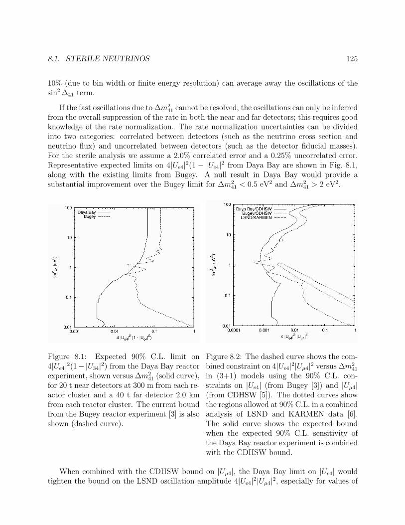
8.1. STERILE NEUTRINOS 125
10% (due to bin width or finite energy resolution) can average away the oscillations of thesin2 ∆41 term.
If the fast oscillations due to ∆m241 cannot be resolved, the oscillations can only be inferred
from the overall suppression of the rate in both the near and far detectors; this requires goodknowledge of the rate normalization. The rate normalization uncertainties can be dividedinto two categories: correlated between detectors (such as the neutrino cross section andneutrino flux) and uncorrelated between detectors (such as the detector fiducial masses).For the sterile analysis we assume a 2.0% correlated error and a 0.25% uncorrelated error.Representative expected limits on 4|Ue4|2(1 − |Ue4|2 from Daya Bay are shown in Fig. 8.1,along with the existing limits from Bugey. A null result in Daya Bay would provide asubstantial improvement over the Bugey limit for ∆m2
41 < 0.5 eV2 and ∆m241 > 2 eV2.
Figure 8.1: Expected 90% C.L. limit on4|Ue4|2(1−|U34|2) from the Daya Bay reactorexperiment, shown versus ∆m2
41 (solid curve),for 20 t near detectors at 300 m from each re-actor cluster and a 40 t far detector 2.0 kmfrom each reactor cluster. The current boundfrom the Bugey reactor experiment [3] is alsoshown (dashed curve).
Figure 8.2: The dashed curve shows the com-bined constraint on 4|Ue4|2|Uµ4|2 versus ∆m2
41
in (3+1) models using the 90% C.L. con-straints on |Ue4| (from Bugey [3]) and |Uµ4|(from CDHSW [5]). The dotted curves showthe regions allowed at 90% C.L. in a combinedanalysis of LSND and KARMEN data [6].The solid curve shows the expected boundwhen the expected 90% C.L. sensitivity ofthe Daya Bay reactor experiment is combinedwith the CDHSW bound.
When combined with the CDHSW bound on |Uµ4|, the Daya Bay limit on |Ue4| wouldtighten the bound on the LSND oscillation amplitude 4|Ue4|2|Uµ4|2, especially for values of
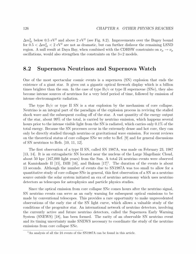
126 CHAPTER 8. OTHER PHYSICS REACHES
∆m241 below 0.5 eV2 and above 2 eV2 (see Fig. 8.2). Improvements over the Bugey bound
for 0.5 < ∆m241 < 2 eV2 are not as dramatic, but can further disfavor the remaining LSND
region. A null result at Daya Bay, when combined with the CDHSW constraints on νµ → νµ
oscillations, would also strengthen the constraints on the 3+2 models.
8.2 Supernova Neutrinos and Supernova Watch
One of the most spectacular cosmic events is a supernova (SN) explosion that ends theexistence of a giant star. It gives out a gigantic optical firework display which is a billiontimes brighter than the sun. In the case of type Ib/c or type II supernovae (SNe), they alsobecome intense sources of neutrinos for a very brief period of time, followed by emission ofintense electromagnetic radiation.
The type Ib/c or type II SN is a star explosion by the mechanism of core collapse.Neutrino is an integral part of the paradigm of the explosion process in reviving the stalledshock wave and the subsequent cooling off of the star. A vast quantity of the energy outputof the star, about 99% of the total, is carried by neutrino emission, which happens severalhours prior to the intense visible light from the SN is radiated, which carries only 0.1% of thetotal energy. Because the SN processes occur in the extremely dense and hot core, they canonly be directly studied through neutrino or gravitational wave emission. For recent reviewson the theoretical status of core collapse SNe we refer to Ref. [9] and for general discussionsof SN neutrinos to Refs. [10, 11, 12].
The first observation of a type II SN, called SN 1987A, was made on February 23, 1987[13, 14]. It is an extragalactic SN located near the nucleus of the Large Magellanic Cloud,about 50 kpc (167,000 light years) from the Sun. A total 24 neutrino events were observedat Kamiokande II [15], IMB [16], and Baksan [17]1. The duration of the events is about13 seconds. Although the number of events due to SN1987A was too small to allow for aquantitative study of core collapse SNe in general, this first observation of a SN as a neutrinosource outside the solar system initiated an era of neutrino astronomy which uses neutrinodetectors as telescopes for astrophysics and particle physics studies.
Since the optical emission from core collapse SNe comes hours after the neutrino signal,SN neutrino events can serve as an early warning for subsequent optical emissions to bemade by conventional telescopes. This provides a rare opportunity to make unprecedentedobservations of the early rise of the SN light curve, which allows a valuable study of theconditions of the progenitor star. An international network of neutrino detectors, involvingthe currently active and future neutrino detectors, called the Supernova Early WarningSystem (SNEWS) [18], has been formed. The rarity of an observable SN neutrino eventand its timing uncertainty make SNEWS necessary to coordinate the study of the neutrinoemissions from core collapse SNe.
1An analysis of all the 24 events of the SN1987A can be found in this article.
8.2. SUPERNOVA NEUTRINOS AND SUPERNOVA WATCH 127
8.2.1 SN neutrino spectra and flux
The SN neutrino parameters are generally model dependent, relying on the details of thecore collapse mechanism which determines the total energy release, and the mode of neutrinoproduction and transport. Since all of these are based on general physics arguments and well-established particle and nuclear physics reactions, their general validity is expected, unlessvery different physics would appear in a high temperature and high density environment.We summarize the spectra of the neutrino produced in a SN as follows:
• Neutrino spectra: Neutrino spectra can be approximately described by Fermi-Diracdistributions [19]. For neutrinos of flavor α, the time-integrated spectra are given by
F (0)α (E) =
L(0)α
F3T 4α
E2
exp(E/Tα) + 1, (8.2)
where E and Tα are the energy and effective temperature of να, L(0)α is its total lu-
minosity, and F3 = 7π4/120. The average neutrino energy is E(0)α = 3.15Tα. The
neutrino temperatures are hierarchical: Tνe < Tνe < Tνx , hence are their average ener-
gies: E(0)νe
< E(0)νe
< E(0)νx
, where νx denotes νµ, νµ, ντ , or ντ which behave similarly inSN. The total number of neutrino of flavor α is given by
N (0)α =
L(0)α
E(0)α
. (8.3)
• Neutrino luminosity: The simplest argument of the production of neutrinos in thecooling core leads to the equipartition of energy among all six species of neutrinos andantineutrinos (although there are other possibilities). Therefore they are produced withthe same luminosity when emerged from the SN, that is, Lνe ≈ Lνe ≈ Lνx [19, 20]2.Then
L(0)α =
0.99
6E
(0)SN, (8.4)
where E(0)SN is the total energy released in the SN explosion. The numbers of neutrinos of
different flavors emitted by SN also satisfy the hierarchical relation N (0)νe
> N(0)νe
> N (0)νx
.
The oscillation effect is important in determining the detailed features of SN neutrinosthat are detected by terrestrial detectors, such as the total number of each flavor and theirenergy distributions. To do a detailed study requires a large number of events. The SNEWSnetwork can be useful, especially some of the SNEWS detectors can provide the directionalinformation of the SN event to determine the extent of the Earth matter effect.
2There are other possibilities. It is generally expected to be true that Lνe ≈ Lνe and Lx ≡ Lνµ ≈ Lνµ ≈Lντ ≈ Lντ . However Lνe and Lx can differ by a factor 2, Lx = (0.5− 2)Lνe .
128 CHAPTER 8. OTHER PHYSICS REACHES
At their production, SN neutrinos are in a very high density environment of ρ ∼ 1011 g/cm3.The matter effect dominates the Hamiltonian of the neutrino system and hence the flavoreigenstates coincide with the mass eigenstates. Propagating outward from their produc-tion point deep inside the SN, the neutrinos and antineutrinos experience a continuouslydecreasing matter density which goes to zero at the SN surface. Hence the neutrinos andantineutrinos are subjected to the MSW resonance effect and level crossing [21, 22].
The treatment of the SN matter effect is similar to that of the Sun. While there isonly one MSW resonance in the Sun, SNe have two MSW resonances. With the solar LMAsolution, neutrinos and antineutrinos can have at most only one level crossing. For neutrinos,it is the usual resonance for the solar neutrinos (involving the neutrino parameters ∆m2
21
and sin2 2θ12). For antineutrinos, a resonance only occurs for the inverted mass hierarchy(involving ∆m2
31 and sin2 2θ13). A detailed treatment of the SN matter effect can be foundin [10] which we follow in our calculations below.
Before a SN neutrino enters a detector it may go through part of the Earth and thereforemay be subjected to the Earth matter regeneration effect. Depending on the direction ofthe incoming SN neutrinos, the amount of Earth matter traversed varies from the heightof the overburden of a detector to the whole Earth diameter. Unlike the SN matter effect,the Earth matter effect cannot be specified, a priori, before the direction of the SN event isknown. The Earth matter effect is generally of second order. Details of the treatment of theEarth matter effect can be found in Refs. [10] and [23].
The effects of the oscillation and the level crossing depend on the mixing angles θ12
and θ13. Due to the smallness of θ13 and the SN model uncertainties, we will ignore theterms dependent on θ13. The SN neutrino fluxes arriving on Earth (not including the Earthmatter effect), expressed in terms of the neutrino fluxes originally produced in the SN, aresummarized as follows:
• SN matter effect for the normal mass hierarchy, ∆m231 > 0,
F (N)νe
≈ PH sin2 θ12F(0)νe
+ (1− PH sin2 θ12)F(0)νx
(8.5)
F(N)νe
≈ cos2 θ12F(0)νe
+ sin2 θ12F(0)νx
2F (N)νx
≈ (1− PH sin2 θ12)F(0)νe
+ (1 + PH sin2 θ12)F(0)νx
2F(N)νx
≈ sin2 θ12F(0)νe
+ (1 + cos2 θ12)F(0)νx
• SN matter effect for the inverted mass hierarchy, ∆m231 < 0
F (I)νe
≈ sin2 θ12F(0)νe
+ cos2 θ12F(0)νx
(8.6)
F(I)νe
≈ PH cos2 θ12F(0)νe
+ (1− PH cos2 θ12)F(0)νx
2F (I)νx
≈ cos2 θ12F(0)νe
+ (1 + sin2 θ12)F(0)νx
2F(I)νx
≈ (1− PH cos2 θ12)F(0)νe
+ (1 + PH cos2 θ12)F(0)νx
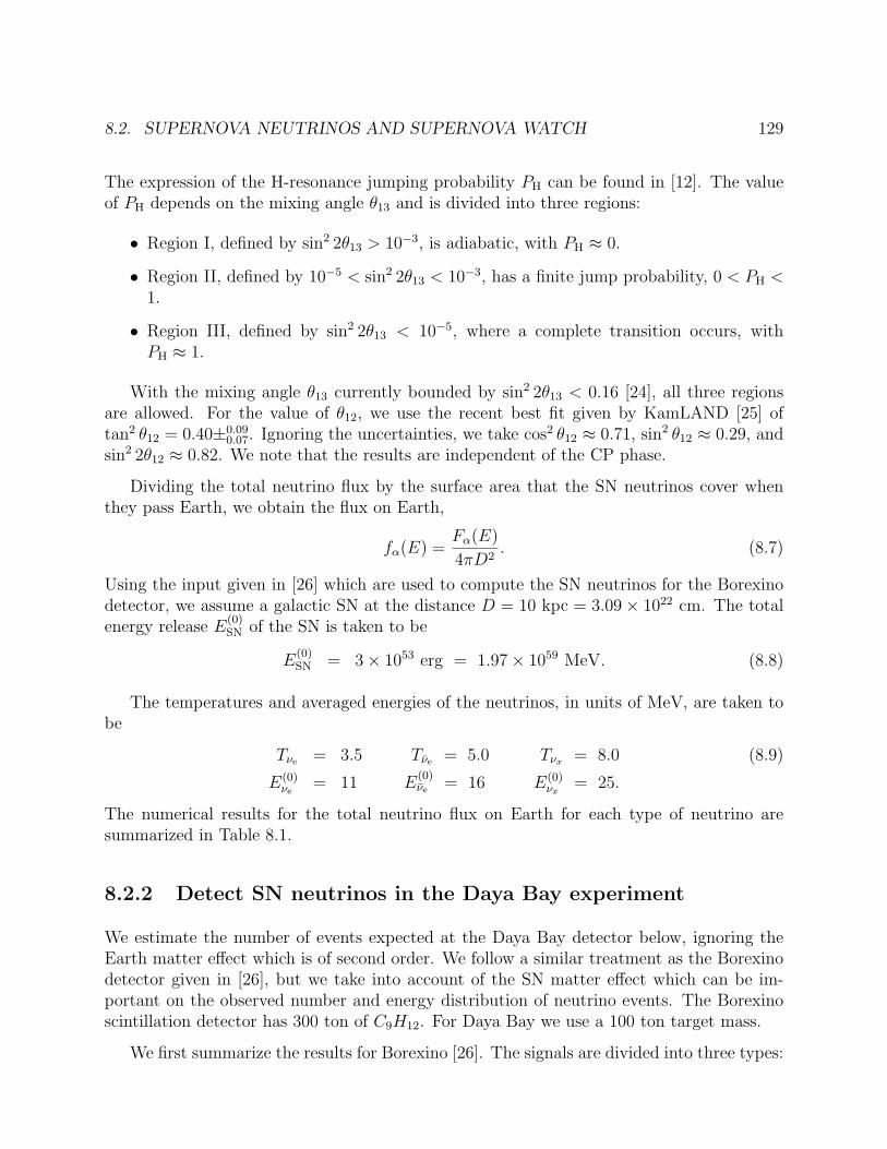
8.2. SUPERNOVA NEUTRINOS AND SUPERNOVA WATCH 129
The expression of the H-resonance jumping probability PH can be found in [12]. The valueof PH depends on the mixing angle θ13 and is divided into three regions:
• Region I, defined by sin2 2θ13 > 10−3, is adiabatic, with PH ≈ 0.
• Region II, defined by 10−5 < sin2 2θ13 < 10−3, has a finite jump probability, 0 < PH <1.
• Region III, defined by sin2 2θ13 < 10−5, where a complete transition occurs, withPH ≈ 1.
With the mixing angle θ13 currently bounded by sin2 2θ13 < 0.16 [24], all three regionsare allowed. For the value of θ12, we use the recent best fit given by KamLAND [25] oftan2 θ12 = 0.40±0.09
0.07. Ignoring the uncertainties, we take cos2 θ12 ≈ 0.71, sin2 θ12 ≈ 0.29, andsin2 2θ12 ≈ 0.82. We note that the results are independent of the CP phase.
Dividing the total neutrino flux by the surface area that the SN neutrinos cover whenthey pass Earth, we obtain the flux on Earth,
fα(E) =Fα(E)
4πD2. (8.7)
Using the input given in [26] which are used to compute the SN neutrinos for the Borexinodetector, we assume a galactic SN at the distance D = 10 kpc = 3.09× 1022 cm. The totalenergy release E
(0)SN of the SN is taken to be
E(0)SN = 3× 1053 erg = 1.97× 1059 MeV. (8.8)
The temperatures and averaged energies of the neutrinos, in units of MeV, are taken tobe
Tνe = 3.5 Tνe = 5.0 Tνx = 8.0 (8.9)
E(0)νe
= 11 E(0)νe
= 16 E(0)νx
= 25.
The numerical results for the total neutrino flux on Earth for each type of neutrino aresummarized in Table 8.1.
8.2.2 Detect SN neutrinos in the Daya Bay experiment
We estimate the number of events expected at the Daya Bay detector below, ignoring theEarth matter effect which is of second order. We follow a similar treatment as the Borexinodetector given in [26], but we take into account of the SN matter effect which can be im-portant on the observed number and energy distribution of neutrino events. The Borexinoscintillation detector has 300 ton of C9H12. For Daya Bay we use a 100 ton target mass.
We first summarize the results for Borexino [26]. The signals are divided into three types:
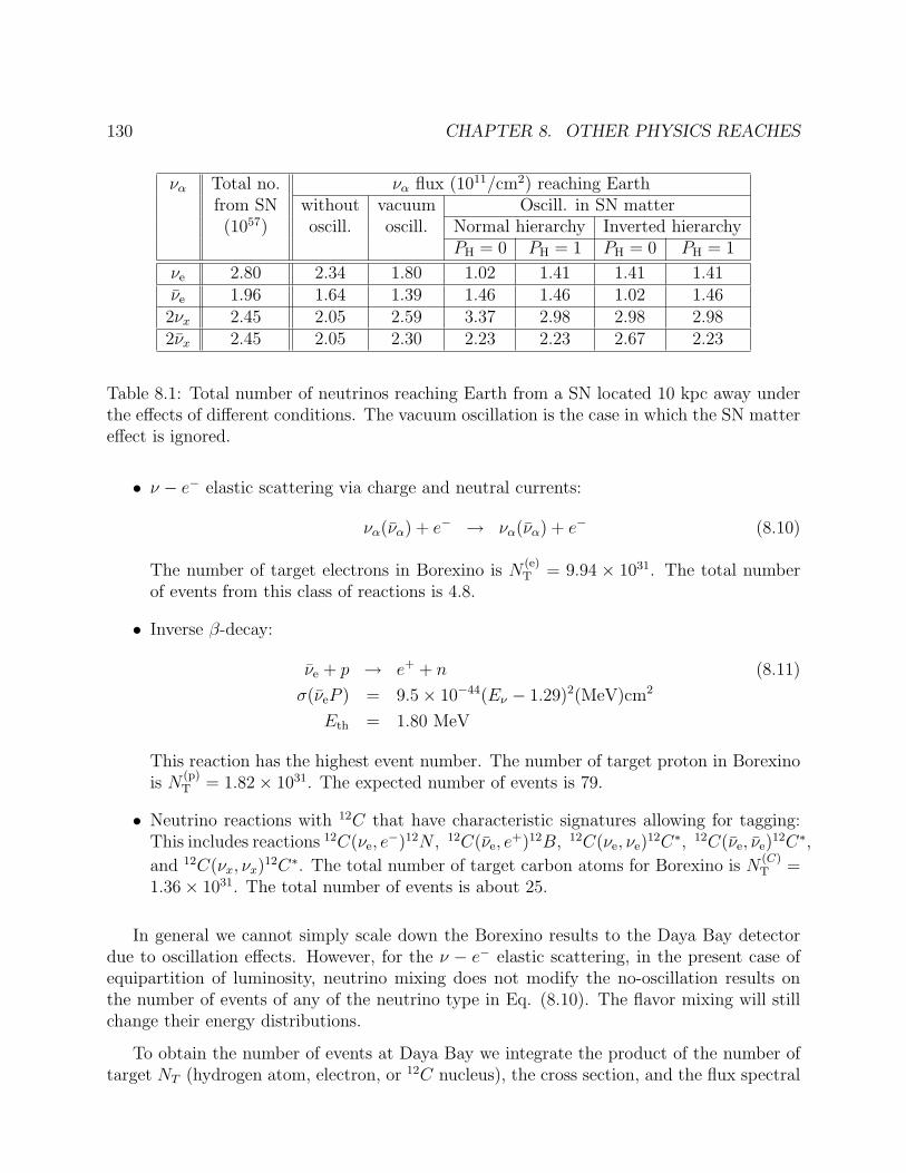
130 CHAPTER 8. OTHER PHYSICS REACHES
να Total no. να flux (1011/cm2) reaching Earthfrom SN without vacuum Oscill. in SN matter(1057) oscill. oscill. Normal hierarchy Inverted hierarchy
PH = 0 PH = 1 PH = 0 PH = 1
νe 2.80 2.34 1.80 1.02 1.41 1.41 1.41νe 1.96 1.64 1.39 1.46 1.46 1.02 1.462νx 2.45 2.05 2.59 3.37 2.98 2.98 2.982νx 2.45 2.05 2.30 2.23 2.23 2.67 2.23
Table 8.1: Total number of neutrinos reaching Earth from a SN located 10 kpc away underthe effects of different conditions. The vacuum oscillation is the case in which the SN mattereffect is ignored.
• ν − e− elastic scattering via charge and neutral currents:
να(να) + e− → να(να) + e− (8.10)
The number of target electrons in Borexino is N(e)T = 9.94 × 1031. The total number
of events from this class of reactions is 4.8.
• Inverse β-decay:
νe + p → e+ + n (8.11)
σ(νeP ) = 9.5× 10−44(Eν − 1.29)2(MeV)cm2
Eth = 1.80 MeV
This reaction has the highest event number. The number of target proton in Borexinois N
(p)T = 1.82× 1031. The expected number of events is 79.
• Neutrino reactions with 12C that have characteristic signatures allowing for tagging:This includes reactions 12C(νe, e
−)12N , 12C(νe, e+)12B, 12C(νe, νe)
12C∗, 12C(νe, νe)12C∗,
and 12C(νx, νx)12C∗. The total number of target carbon atoms for Borexino is N
(C)T =
1.36× 1031. The total number of events is about 25.
In general we cannot simply scale down the Borexino results to the Daya Bay detectordue to oscillation effects. However, for the ν − e− elastic scattering, in the present case ofequipartition of luminosity, neutrino mixing does not modify the no-oscillation results onthe number of events of any of the neutrino type in Eq. (8.10). The flavor mixing will stillchange their energy distributions.
To obtain the number of events at Daya Bay we integrate the product of the number oftarget NT (hydrogen atom, electron, or 12C nucleus), the cross section, and the flux spectral
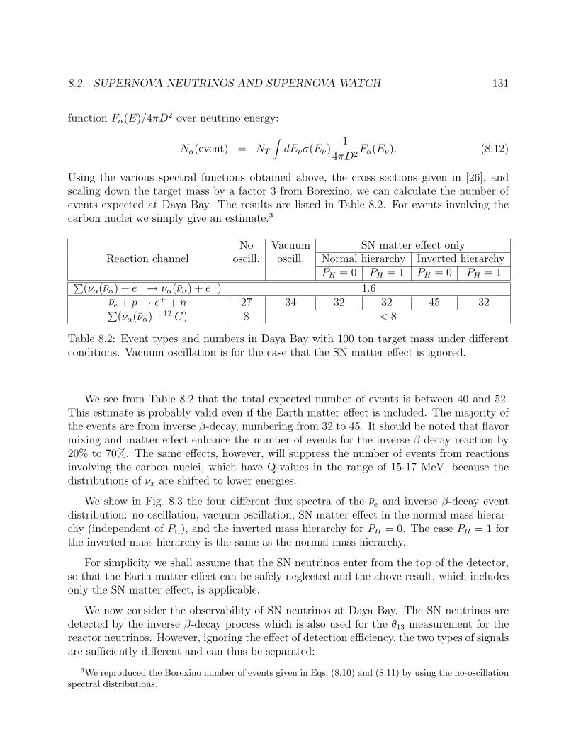
8.2. SUPERNOVA NEUTRINOS AND SUPERNOVA WATCH 131
function Fα(E)/4πD2 over neutrino energy:
Nα(event) = NT
∫dEνσ(Eν)
1
4πD2Fα(Eν). (8.12)
Using the various spectral functions obtained above, the cross sections given in [26], andscaling down the target mass by a factor 3 from Borexino, we can calculate the number ofevents expected at Daya Bay. The results are listed in Table 8.2. For events involving thecarbon nuclei we simply give an estimate.3
No Vacuum SN matter effect onlyReaction channel oscill. oscill. Normal hierarchy Inverted hierarchy
PH = 0 PH = 1 PH = 0 PH = 1∑
(να(να) + e− → να(να) + e−) 1.6νe + p → e+ + n 27 34 32 32 45 32∑
(να(να) +12 C) 8 < 8
Table 8.2: Event types and numbers in Daya Bay with 100 ton target mass under differentconditions. Vacuum oscillation is for the case that the SN matter effect is ignored.
We see from Table 8.2 that the total expected number of events is between 40 and 52.This estimate is probably valid even if the Earth matter effect is included. The majority ofthe events are from inverse β-decay, numbering from 32 to 45. It should be noted that flavormixing and matter effect enhance the number of events for the inverse β-decay reaction by20% to 70%. The same effects, however, will suppress the number of events from reactionsinvolving the carbon nuclei, which have Q-values in the range of 15-17 MeV, because thedistributions of νx are shifted to lower energies.
We show in Fig. 8.3 the four different flux spectra of the νe and inverse β-decay eventdistribution: no-oscillation, vacuum oscillation, SN matter effect in the normal mass hierar-chy (independent of PH), and the inverted mass hierarchy for PH = 0. The case PH = 1 forthe inverted mass hierarchy is the same as the normal mass hierarchy.
For simplicity we shall assume that the SN neutrinos enter from the top of the detector,so that the Earth matter effect can be safely neglected and the above result, which includesonly the SN matter effect, is applicable.
We now consider the observability of SN neutrinos at Daya Bay. The SN neutrinos aredetected by the inverse β-decay process which is also used for the θ13 measurement for thereactor neutrinos. However, ignoring the effect of detection efficiency, the two types of signalsare sufficiently different and can thus be separated:
3We reproduced the Borexino number of events given in Eqs. (8.10) and (8.11) by using the no-oscillationspectral distributions.
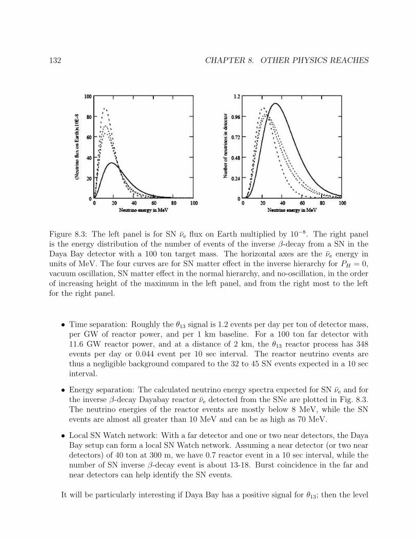
132 CHAPTER 8. OTHER PHYSICS REACHES
Figure 8.3: The left panel is for SN νe flux on Earth multiplied by 10−8. The right panelis the energy distribution of the number of events of the inverse β-decay from a SN in theDaya Bay detector with a 100 ton target mass. The horizontal axes are the νe energy inunits of MeV. The four curves are for SN matter effect in the inverse hierarchy for PH = 0,vacuum oscillation, SN matter effect in the normal hierarchy, and no-oscillation, in the orderof increasing height of the maximum in the left panel, and from the right most to the leftfor the right panel.
• Time separation: Roughly the θ13 signal is 1.2 events per day per ton of detector mass,per GW of reactor power, and per 1 km baseline. For a 100 ton far detector with11.6 GW reactor power, and at a distance of 2 km, the θ13 reactor process has 348events per day or 0.044 event per 10 sec interval. The reactor neutrino events arethus a negligible background compared to the 32 to 45 SN events expected in a 10 secinterval.
• Energy separation: The calculated neutrino energy spectra expected for SN νe and forthe inverse β-decay Dayabay reactor νe detected from the SNe are plotted in Fig. 8.3.The neutrino energies of the reactor events are mostly below 8 MeV, while the SNevents are almost all greater than 10 MeV and can be as high as 70 MeV.
• Local SN Watch network: With a far detector and one or two near detectors, the DayaBay setup can form a local SN Watch network. Assuming a near detector (or two neardetectors) of 40 ton at 300 m, we have 0.7 reactor event in a 10 sec interval, while thenumber of SN inverse β-decay event is about 13-18. Burst coincidence in the far andnear detectors can help identify the SN events.
It will be particularly interesting if Daya Bay has a positive signal for θ13; then the level
8.3. EXOTIC NEUTRINO PROPERTIES AND NUCLEAR POWER MONITORING133
crossing is in region I and the flip probability will be PH = 0. The normal and inverted masshierarchies are expected to have, respectively, 32 and 45 inverse β-decay events in the fardetector from the SN, providing a way to distinguish between the two hierachies.
8.3 Exotic neutrino properties and nuclear power mon-
itoring
The measurement of θ13 as discussed in the present work initiates an era of precision mea-surement of neutrino physics and the study of more details of the properties of neutrinos canbe expected in the future. Several questions on neutrinos that seem to be exotic are validinquiries based on theoretical expectations. Hence it is important to investigate them whenopportunities arise. Any positive signal of them could mean a revolutionary discovery whichcould open completely new doors for rethinking the structure of particle physics. Thesequestions include the sterile neutrinos, the neutrino magnetic moment, and exotic interac-tions of neutrinos of possibly flavor changing type. To answer these questions requires avery high intensity neutrino beam and suitable detectors. These could be naturally achievedwith an extension of the Daya Bay experiment by suitably designing an experimental hallconstructed very closely to one of the reactor cores of the the Ling Ao II reactors whichare currently under construction. For example, a detector made of high purity germaniumcrystals can double as a monitor of the reactor power with a accuracy better than what iscurrently available from the nuclear power industry. Detailed physics simulations and thedetector design could be made if the opportunity arises.
Bibliography
[1] C. Athanassopoulos et al. [LSND Collaboration], Phys. Rev. C 54, 2685 (1996)[arXiv:nucl-ex/9605001]; Phys. Rev. Lett. 77, 3082 (1996) [arXiv:nucl-ex/9605003];A. Aguilar et al., Phys. Rev. D 64, 112007 (2001) [arXiv:hep-ex/0104049].
[2] B. Armbruster et al. [KARMEN Collaboration], Phys. Rev. C 57, 3414 (1998)[arXiv:hep-ex/9801007]; Phys. Rev. D 65, 112001 (2002) [arXiv:hep-ex/0203021].
[3] Y. Declais et al., Phys. Lett. B338, 383 (1994); B. Ackar et al., Nucl. Phys. B434, 503(1995); B. Ackar et al., Phys. Lett. B374, 243 (1996).
[4] M. Maltoni, T. Schwetz, M. A. Tortola and J. W. Valle, Nucl. Phys. B 643, 321 (2002)[arXiv:hep-ph/0207157]; Phys. Rev. D 67, 013011 (2003) [arXiv:hep-ph/0207227].
[5] F. Dydak et al., Phys. Lett. B 134, 281 (1984).
[6] E. D. Church, K. Eitel, G. B. Mills and M. Steidl, Phys. Rev. D 66, 013001 (2002)[arXiv:hep-ex/0203023].
[7] M. Sorel, J. Conrad and M. Shaevitz, Phys. Rev. D 70, 073004 (2004) [arXiv:hep-ph/0305255].
[8] V. Barger, D. Marfatia and K. Whisnant, Phys. Lett. B 576, 303 (2003) [arXiv:hep-ph/0308299].
[9] A. Mezzacappa, The core collapse supernova mechanism: current models, gaps, and theroad ahead, arXiv:astro-ph/0410085.
[10] A.S. Dighe and A.Y. Smirnov, Phys. Rev. D62, 033007 (2000) [arXiv:hep-ph/9907423].
[11] A. Dighe, Supernova neutrinos: production, propagation and oscillations, talk given inneutrino 2004, arXiv:hep-ph/0409268.
[12] C. Lunardini, Physics of Supernova Neutrinos, Proceedings, International Workshop onAstroparticle and High Energy Physics, Valencia, Spain, 14-18, 2003 (IHEP2003/043).
134

BIBLIOGRAPHY 135
[13] D. Schramm, Neutrinos from supernova 1987A, Fermilab Report: FERMILAB-pub-87/91-A.
[14] T.K. Kuo and J. Pantaleone, Rev. Mod. Phys. 61, 937 (1989).
[15] [Kamiokande II] K. Hirata et al., Phys. Rev. Lett. 58, 1490 (1987).
[16] [IMB] R.M. Bionta et al., Phys. Rev. Lett. 58, 1494 (1987).
[17] [Baksan] E.N. Alexevey, et al., Phys. Lett. B205 (1988) 209.
[18] [SNEWS] P. Antonioli et al., SNEWS: The SuperNova Early Warning System,arXiv:astro-ph/0406214; K. Scholberg, Supernova Neutrino Detection, 19th Inter-national Conference on Neutrino Physics (Neutrino 2000), Sudbery Ontario, 2000[arXiv:hep-ex/0008044].
[19] T. Totani, K. Sato, H.E. Dalhed, and J.R. Wilson, Astophys. J. 496, 216 (1998)[arXiv:astro-ph/9710203].
[20] K. Langanke, P. Vogel, and E. Kolbe, Phys. Rev. Lett., 76, 2629 (1996) [arXiv:nucl-th/9511032].
[21] L. Wolfenstein, Phys. Rev. 17 2369 (1979).
[22] S.P. Mikheyev and A.Yu. Smirnov, Sov. J. Nucl. Phys. 42, 913 (1985); Nuovo CimentoC9, 17 (1986).
[23] A.N. Ioannisian, N.A. Kazarian, A.Yu. Smirnov, and D. Wyler, Phys. Rev. D 71, 033006(2005) [arXiv:hep-ph/0407138].
[24] [Chooz] M. Apollonio et al., Phys. Lett., B466, 415 (1999) (arXiv:hep-ex/9907037).
[25] [KamLAND] T. Araki et al., Phys. Rev. Lett. 94, 081801 (2005) [arXiv:hep-ex/0406035].
[26] L. Cadonati, F.P. Calaprice, and M.C. Chen, Astropart. Phys. 16, 361 (2002)[arXiv:hep-ph/0012082].

136 BIBLIOGRAPHY
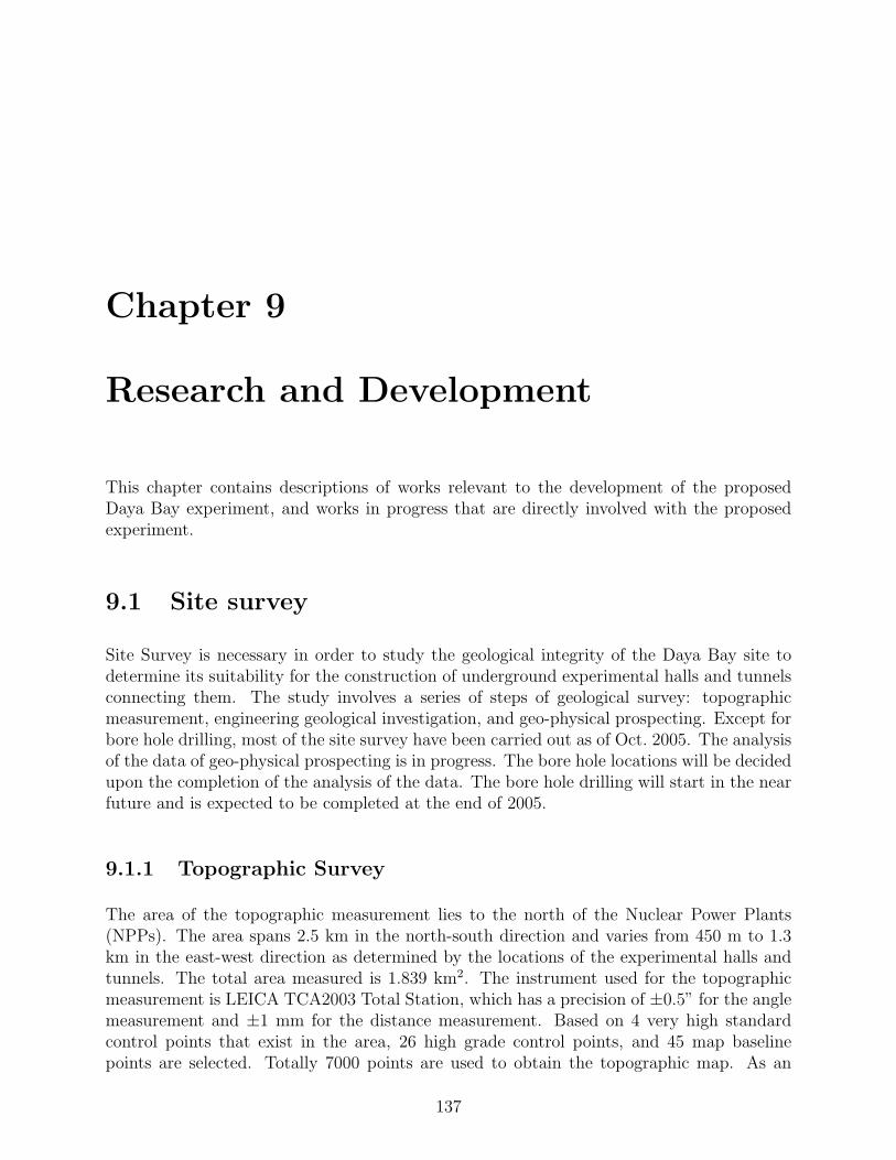
Chapter 9
Research and Development
This chapter contains descriptions of works relevant to the development of the proposedDaya Bay experiment, and works in progress that are directly involved with the proposedexperiment.
9.1 Site survey
Site Survey is necessary in order to study the geological integrity of the Daya Bay site todetermine its suitability for the construction of underground experimental halls and tunnelsconnecting them. The study involves a series of steps of geological survey: topographicmeasurement, engineering geological investigation, and geo-physical prospecting. Except forbore hole drilling, most of the site survey have been carried out as of Oct. 2005. The analysisof the data of geo-physical prospecting is in progress. The bore hole locations will be decidedupon the completion of the analysis of the data. The bore hole drilling will start in the nearfuture and is expected to be completed at the end of 2005.
9.1.1 Topographic Survey
The area of the topographic measurement lies to the north of the Nuclear Power Plants(NPPs). The area spans 2.5 km in the north-south direction and varies from 450 m to 1.3km in the east-west direction as determined by the locations of the experimental halls andtunnels. The total area measured is 1.839 km2. The instrument used for the topographicmeasurement is LEICA TCA2003 Total Station, which has a precision of ±0.5” for the anglemeasurement and ±1 mm for the distance measurement. Based on 4 very high standardcontrol points that exist in the area, 26 high grade control points, and 45 map baselinepoints are selected. Totally 7000 points are used to obtain the topographic map. As an
137
138 CHAPTER 9. RESEARCH AND DEVELOPMENT
example, Fig. 9.1 shows the topographic map around the far site, scaled by 1:2000. Thealtitude difference between adjacent contour lines is one meter. The area around the mainportal, which is behind a local hospital, and two possible construction portals are measuredin a higher scale of 1:500. The cross sections along the tunnel line for each of the constructionportals are measured in an even higher scale of 1:200. The positions of the experimentalhalls, the main portal, and the construction portals are marked on the topographic map.
Figure 9.1: The topography map around the far site. The location of the far detector ismarked by a red square in the middle of the map.
9.1.2 Geological investigation
The geological survey has been conducted in an area about 2.5 km in the north-south direc-tion and about 3 km in the east-west direction, as shown in Fig. 9.2. The survey includesall the areas passed through by the tunnels and occupied by the four experimental halls.
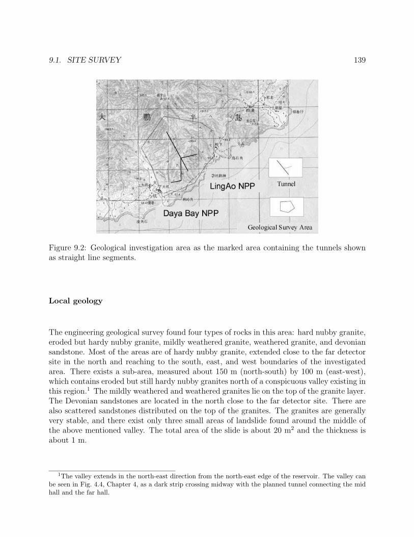
9.1. SITE SURVEY 139
Figure 9.2: Geological investigation area as the marked area containing the tunnels shownas straight line segments.
Local geology
The engineering geological survey found four types of rocks in this area: hard nubby granite,eroded but hardy nubby granite, mildly weathered granite, weathered granite, and devoniansandstone. Most of the areas are of hardy nubby granite, extended close to the far detectorsite in the north and reaching to the south, east, and west boundaries of the investigatedarea. There exists a sub-area, measured about 150 m (north-south) by 100 m (east-west),which contains eroded but still hardy nubby granites north of a conspicuous valley existing inthis region.1 The mildly weathered and weathered granites lie on the top of the granite layer.The Devonian sandstones are located in the north close to the far detector site. There arealso scattered sandstones distributed on the top of the granites. The granites are generallyvery stable, and there exist only three small areas of landslide found around the middle ofthe above mentioned valley. The total area of the slide is about 20 m2 and the thickness isabout 1 m.
1The valley extends in the north-east direction from the north-east edge of the reservoir. The valley canbe seen in Fig. 4.4, Chapter 4, as a dark strip crossing midway with the planned tunnel connecting the midhall and the far hall.
140 CHAPTER 9. RESEARCH AND DEVELOPMENT
Underground water
The accumulation and distribution of underground water depend generally on the localclimate, hydrology, landform, lithology of stratum, and detailed geological structure. ForDaya Bay, in the investigated area, the amount of underground water flux depends, in acomplicated way, on the atmospheric precipitation and the underground water seeping thatoccurs. The sandstone area is rich in underground water seeping in mainly through jointsdue to weathering of crannies formed in the structure. No circulation is found between theunderground water and outside boundary water in this area. Underground water mainlycomes from the atmospheric precipitation, and they emerge in the low land and are then fedto the ocean.
9.1.3 Geo-physical prospecting
Three methods are commonly used in geo-physical prospecting, i.e., the high density electri-cal resistivity method, the high resolution gravity method, and the seismic refraction imagemethod using mechanical hammer. The first two methods together with the third as sup-plement have been used for the Daya Bay prospecting.2 Figure 9.3 shows the sections thatare subject to geo-physical survey, including all tunnels and experimental halls. The exper-imental halls are marked explicitly in Fig. 9.3, and the lines being measured are labelled asA, A1, A2, B, B1, C, D, E1, E2, and F. Depending on the characteristics of the granite andits geological structure, the electrical resistivity of this area can vary from tens of ohm-mto more than 10k ohm-m. The non-weathered granite has the highest electrical resistivity,whereas the sandstone has medium resistivity due to trapped moisture. The weathered zone,consisting of weathered bursa and faults, has relatively low resistivity. Figure 9.4 shows theelectrical resistivity measurement from the construction portal to the mid-hall marked asline C in Fig. 9.3. A detailed analysis of the geo-physical prospecting data is in progress.
2In order not to affect the construction work of Ling Ao II, heavy blaster as a source of the seismicrefraction measurement, as required for deep underground measurement, cannot be used. Therefore seismicrefraction cannot be used as a major tool for the Daya Bay prospecting.
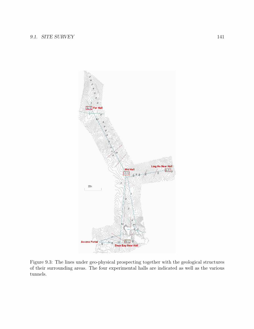
9.1. SITE SURVEY 141
Figure 9.3: The lines under geo-physical prospecting together with the geological structuresof their surrounding areas. The four experimental halls are indicated as well as the varioustunnels.
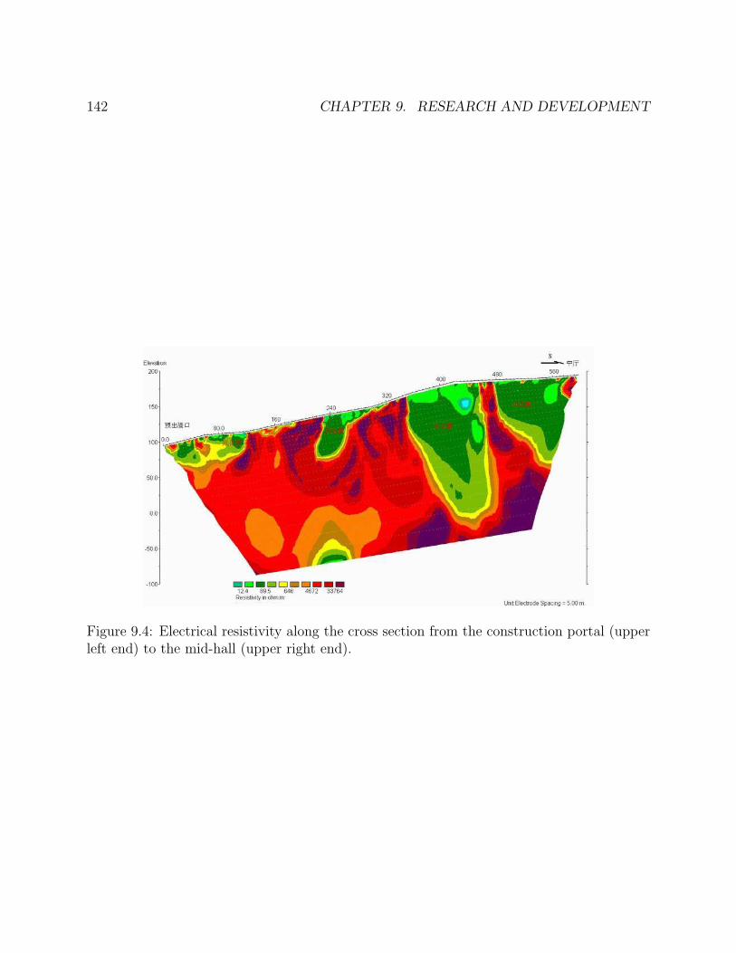
142 CHAPTER 9. RESEARCH AND DEVELOPMENT
Figure 9.4: Electrical resistivity along the cross section from the construction portal (upperleft end) to the mid-hall (upper right end).
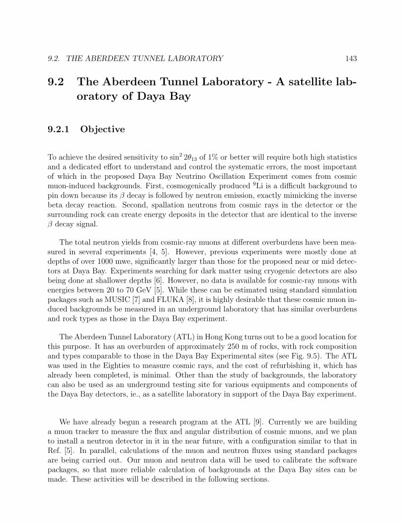
9.2. THE ABERDEEN TUNNEL LABORATORY 143
9.2 The Aberdeen Tunnel Laboratory - A satellite lab-
oratory of Daya Bay
9.2.1 Objective
To achieve the desired sensitivity to sin2 2θ13 of 1% or better will require both high statisticsand a dedicated effort to understand and control the systematic errors, the most importantof which in the proposed Daya Bay Neutrino Oscillation Experiment comes from cosmicmuon-induced backgrounds. First, cosmogenically produced 9Li is a difficult background topin down because its β decay is followed by neutron emission, exactly mimicking the inversebeta decay reaction. Second, spallation neutrons from cosmic rays in the detector or thesurrounding rock can create energy deposits in the detector that are identical to the inverseβ decay signal.
The total neutron yields from cosmic-ray muons at different overburdens have been mea-sured in several experiments [4, 5]. However, previous experiments were mostly done atdepths of over 1000 mwe, significantly larger than those for the proposed near or mid detec-tors at Daya Bay. Experiments searching for dark matter using cryogenic detectors are alsobeing done at shallower depths [6]. However, no data is available for cosmic-ray muons withenergies between 20 to 70 GeV [5]. While these can be estimated using standard simulationpackages such as MUSIC [7] and FLUKA [8], it is highly desirable that these cosmic muon in-duced backgrounds be measured in an underground laboratory that has similar overburdensand rock types as those in the Daya Bay experiment.
The Aberdeen Tunnel Laboratory (ATL) in Hong Kong turns out to be a good location forthis purpose. It has an overburden of approximately 250 m of rocks, with rock compositionand types comparable to those in the Daya Bay Experimental sites (see Fig. 9.5). The ATLwas used in the Eighties to measure cosmic rays, and the cost of refurbishing it, which hasalready been completed, is minimal. Other than the study of backgrounds, the laboratorycan also be used as an underground testing site for various equipments and components ofthe Daya Bay detectors, ie., as a satellite laboratory in support of the Daya Bay experiment.
We have already begun a research program at the ATL [9]. Currently we are buildinga muon tracker to measure the flux and angular distribution of cosmic muons, and we planto install a neutron detector in it in the near future, with a configuration similar to that inRef. [5]. In parallel, calculations of the muon and neutron fluxes using standard packagesare being carried out. Our muon and neutron data will be used to calibrate the softwarepackages, so that more reliable calculation of backgrounds at the Daya Bay sites can bemade. These activities will be described in the following sections.
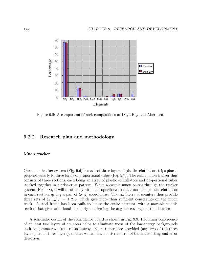
144 CHAPTER 9. RESEARCH AND DEVELOPMENT
Figure 9.5: A comparison of rock compositions at Daya Bay and Aberdeen.
9.2.2 Research plan and methodology
Muon tracker
Our muon tracker system (Fig. 9.6) is made of three layers of plastic scintillator strips placedperpendicularly to three layers of proportional tubes (Fig. 9.7). The entire muon tracker thusconsists of three sections, each being an array of plastic scintillators and proportional tubesstacked together in a criss-cross pattern. When a cosmic muon passes through the trackersystem (Fig. 9.8), it will most likely hit one proportional counter and one plastic scintillatorin each section, giving a pair of (x, y) coordinates. The six layers of counters thus providethree sets of (xi, yi), i = 1, 2, 3, which give more than sufficient constraints on the muontrack. A steel frame has been built to house the entire detector, with a movable middlesection that gives additional flexibility in selecting the angular coverage of the detector.
A schematic design of the coincidence board is shown in Fig. 9.9. Requiring coincidenceof at least two layers of counters helps to eliminate most of the low-energy backgroundssuch as gamma-rays from rocks nearby. Four triggers are provided (any two of the threelayers plus all three layers), so that we can have better control of the track fitting and errordetection.
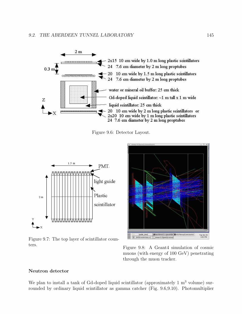
9.2. THE ABERDEEN TUNNEL LABORATORY 145
Figure 9.6: Detector Layout.
Figure 9.7: The top layer of scintillator coun-ters.
Figure 9.8: A Geant4 simulation of cosmicmuons (with energy of 100 GeV) penetratingthrough the muon tracker.
Neutron detector
We plan to install a tank of Gd-doped liquid scintillator (approximately 1 m3 volume) sur-rounded by ordinary liquid scintillator as gamma catcher (Fig. 9.6,9.10). Photomultiplier
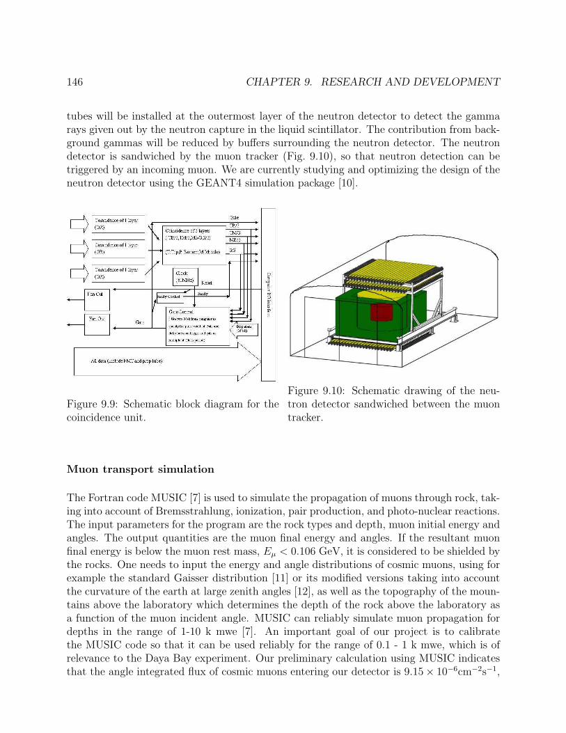
146 CHAPTER 9. RESEARCH AND DEVELOPMENT
tubes will be installed at the outermost layer of the neutron detector to detect the gammarays given out by the neutron capture in the liquid scintillator. The contribution from back-ground gammas will be reduced by buffers surrounding the neutron detector. The neutrondetector is sandwiched by the muon tracker (Fig. 9.10), so that neutron detection can betriggered by an incoming muon. We are currently studying and optimizing the design of theneutron detector using the GEANT4 simulation package [10].
Figure 9.9: Schematic block diagram for thecoincidence unit.
Figure 9.10: Schematic drawing of the neu-tron detector sandwiched between the muontracker.
Muon transport simulation
The Fortran code MUSIC [7] is used to simulate the propagation of muons through rock, tak-ing into account of Bremsstrahlung, ionization, pair production, and photo-nuclear reactions.The input parameters for the program are the rock types and depth, muon initial energy andangles. The output quantities are the muon final energy and angles. If the resultant muonfinal energy is below the muon rest mass, Eµ < 0.106 GeV, it is considered to be shielded bythe rocks. One needs to input the energy and angle distributions of cosmic muons, using forexample the standard Gaisser distribution [11] or its modified versions taking into accountthe curvature of the earth at large zenith angles [12], as well as the topography of the moun-tains above the laboratory which determines the depth of the rock above the laboratory asa function of the muon incident angle. MUSIC can reliably simulate muon propagation fordepths in the range of 1-10 k mwe [7]. An important goal of our project is to calibratethe MUSIC code so that it can be used reliably for the range of 0.1 - 1 k mwe, which is ofrelevance to the Daya Bay experiment. Our preliminary calculation using MUSIC indicatesthat the angle integrated flux of cosmic muons entering our detector is 9.15× 10⁻⁶cm−2s−1,
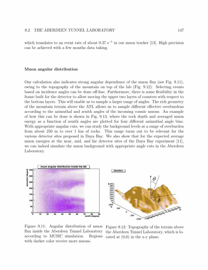
9.2. THE ABERDEEN TUNNEL LABORATORY 147
which translates to an event rate of about 0.37 s−1 in our muon tracker [13]. High precisioncan be achieved with a few months data taking.
Muon angular distribution
Our calculation also indicates strong angular dependence of the muon flux (see Fig. 9.11),owing to the topography of the mountain on top of the lab (Fig. 9.12). Selecting eventsbased on incidence angles can be done off-line. Furthermore, there is some flexibility in theframe built for the detector to allow moving the upper two layers of counters with respect tothe bottom layers. This will enable us to sample a larger range of angles. The rich geometryof the mountain terrain above the ATL allows us to sample different effective overburdensaccording to the azimuthal and zenith angles of the incoming cosmic muons. An exampleof how this can be done is shown in Fig. 9.13, where the rock depth and averaged muonenergy as a function of zenith angles are plotted for four different azimuthal angle bins.With appropriate angular cuts, we can study the background levels at a range of overburdenfrom about 250 m to over 1 km of rocks. This range turns out to be relevant for thevarious detector sites proposed in Daya Bay. We also show that for the expected averagemuon energies at the near, mid, and far detector sites of the Daya Bay experiment [11],we can indeed simulate the muon background with appropriate angle cuts in the AberdeenLaboratory.
Figure 9.11: Angular distribution of muonflux inside the Aberdeen Tunnel Laboratoryaccording to MUSIC simulation. Regionswith darker color receive more muons.
Figure 9.12: Topography of the terrain abovethe Aberdeen Tunnel Laboratory, which is lo-cated at (0,0) in the x-y plane.
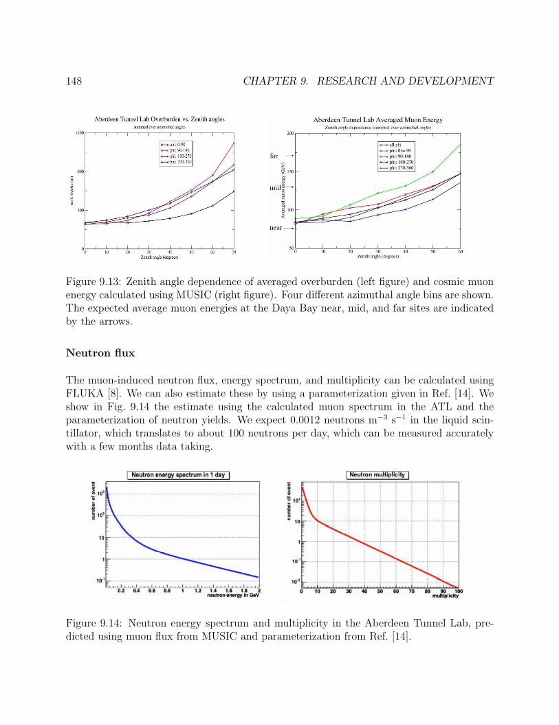
148 CHAPTER 9. RESEARCH AND DEVELOPMENT
Figure 9.13: Zenith angle dependence of averaged overburden (left figure) and cosmic muonenergy calculated using MUSIC (right figure). Four different azimuthal angle bins are shown.The expected average muon energies at the Daya Bay near, mid, and far sites are indicatedby the arrows.
Neutron flux
The muon-induced neutron flux, energy spectrum, and multiplicity can be calculated usingFLUKA [8]. We can also estimate these by using a parameterization given in Ref. [14]. Weshow in Fig. 9.14 the estimate using the calculated muon spectrum in the ATL and theparameterization of neutron yields. We expect 0.0012 neutrons m−3 s−1 in the liquid scin-tillator, which translates to about 100 neutrons per day, which can be measured accuratelywith a few months data taking.
Figure 9.14: Neutron energy spectrum and multiplicity in the Aberdeen Tunnel Lab, pre-dicted using muon flux from MUSIC and parameterization from Ref. [14].

9.2. THE ABERDEEN TUNNEL LABORATORY 149
9.2.3 Anti-Radon painting
To reduce the radon radioactivity in the Aberdeen tunnel laboratory, anti-radon paint hasbeen applied on the walls, as well as other measures such as ventilation and air purification.The paint forms a continuous non-porous membrane on the wall surface. If the paint is thickenough, 222Rn will decay before it can diffuse through the paint. The paint was sprayedonto wall surfaces instead of painting because the wall surface were very rough. Threelayers of paint were applied in total. The radon concentration grows linearly with time ifthe laboratory is closed. The growth rate is measured before, during, and after painting,shown in Fig. 9.15. The measurements are also done under different conditions. The normalcondition has a normal temperature of 23◦C and a normal humidity of 40 - 50%. The highrelative humidity, labelled as ”high RH” on the plot, is 80 - 90%. The high temperature,labelled as ”high temp”, is 38◦C. We found that more than 60% of radon is shielded by theanti-radon paint. The effectiveness of the paint is listed in Table 9.1, where the effectivenessis defined by 1-(Radon level after painting)/(Radon level before painting).
Table 9.1: Effectiveness of radon painting.Conditions Effectiveness
2 layers Normal temperature & humidity (23◦C, 40-50%) 52%High relative humidity (80-90%) 45%
Normal temperature & humidity 66%3 layers High relative humidity 65%
High temperature (38 ◦C) 61%
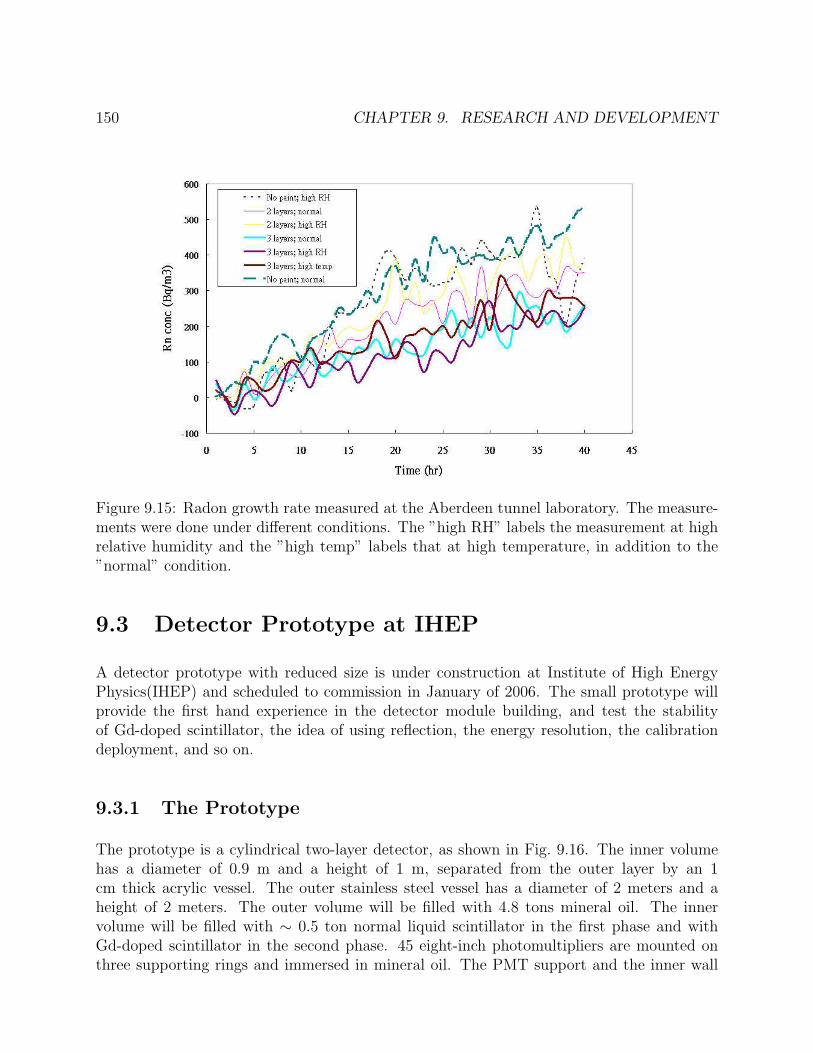
150 CHAPTER 9. RESEARCH AND DEVELOPMENT
Figure 9.15: Radon growth rate measured at the Aberdeen tunnel laboratory. The measure-ments were done under different conditions. The ”high RH” labels the measurement at highrelative humidity and the ”high temp” labels that at high temperature, in addition to the”normal” condition.
9.3 Detector Prototype at IHEP
A detector prototype with reduced size is under construction at Institute of High EnergyPhysics(IHEP) and scheduled to commission in January of 2006. The small prototype willprovide the first hand experience in the detector module building, and test the stabilityof Gd-doped scintillator, the idea of using reflection, the energy resolution, the calibrationdeployment, and so on.
9.3.1 The Prototype
The prototype is a cylindrical two-layer detector, as shown in Fig. 9.16. The inner volumehas a diameter of 0.9 m and a height of 1 m, separated from the outer layer by an 1cm thick acrylic vessel. The outer stainless steel vessel has a diameter of 2 meters and aheight of 2 meters. The outer volume will be filled with 4.8 tons mineral oil. The innervolume will be filled with ∼ 0.5 ton normal liquid scintillator in the first phase and withGd-doped scintillator in the second phase. 45 eight-inch photomultipliers are mounted onthree supporting rings and immersed in mineral oil. The PMT support and the inner wall

9.3. DETECTOR PROTOTYPE AT IHEP 151
of stainless steel vessel are painted in black. At the top and bottom of the outer layer thereare two white-painted reflective acrylic boards. There are two 70 cm long pipes on the topof the acrylic vessel for calibration and liquid filling, one in the middle and the other at theedge. Three LEDs are clung to the outside wall of the acrylic vessel for PMT calibration.
Figure 9.16: The scheme of detector prototype.
The prototype is put inside a muon veto detector. The veto detector is a steel framecovered by plastic scintillators on 5 sides. The frame has a dimension of 3m × 3m × 3m.The top is covered by 20 3-meter-long, 15-cm-wide plastic scintillator strips, which were Timeof Flight (TOF) detector of Beijing Spectrometer (BES). The four sides are each covered by9 quadrate plastic scintillators, 1 m × 1 m in dimension, which are retired from L3+cosmicexperiment. The pictures of prototype detector without and with veto plastic scintillatorare shown in Fig. 9.17.
The scheme of the electronics system for the prototype is shown in Fig. 9.19. The readoutboard is a custom designed 9U VME board that have been described in Section 5.7.2. TheQ signals are processed by a 10-bit 40 MSPS FADC. The charge numerical integration, aswell as T measurement, is implemented in the FPGA. The T and Q data are stored in theevent buffer with a depth of 256 events. The global trigger board is also a custom designed9U VME board which currently provides just one trigger mode, the total energy trigger.That is the sum of charges from all channels. The output of the global trigger is sent tothe muon-veto system that is built with NIM modules. The output signal of the muon-vetosystem is then sent to each of readout boards as a common stop signal. The picture of theelectronics system setup is shown in Fig. 9.18.
The data in each of the readout modules are read out by a VME PowerPC controller, thensent upstream to a Linux PC via LAN. The DAQ software is considered to use a mature
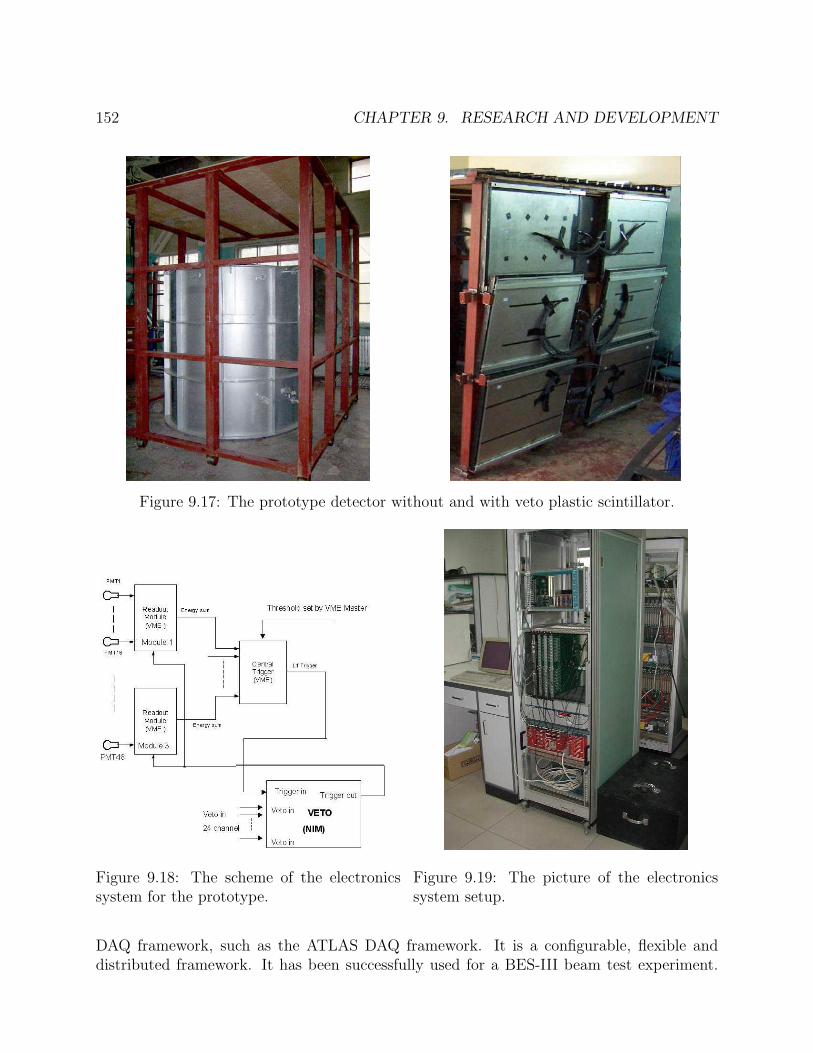
152 CHAPTER 9. RESEARCH AND DEVELOPMENT
Figure 9.17: The prototype detector without and with veto plastic scintillator.
Figure 9.18: The scheme of the electronicssystem for the prototype.
Figure 9.19: The picture of the electronicssystem setup.
DAQ framework, such as the ATLAS DAQ framework. It is a configurable, flexible anddistributed framework. It has been successfully used for a BES-III beam test experiment.
9.3. DETECTOR PROTOTYPE AT IHEP 153
Online system includes data collector, data logout, operation control and histogram display.These tasks will run on a Linux PC while it should be easy to extend to multi VME cratesand multi Linux PCs.
The Hamamatsu R5912 PMT has radioactivity of 5 Bq for 238U, 3 Bq for 252Th, and4.3 Bq for 40K. The distance from the surface of mounted PMTs to the acrylic vessel is 20cm. With the shielding of 20 cm mineral oil and cut at 1 MeV of gamma energy, each PMTcontribute 0.15 Hz for 238U, 0.1 Hz for 252Th, and 0.26 Bq for 40K. The total radioactivityof 45 PMTs is 23 Hz. If cut at 0.5 MeV of gamma energy, the rate will roughly double.The outdoor radon concentration in Beijing is 14.1 ± 5.5 Bq/m3 in average. The radonradioactivity contributes around 80 Hz. Radioactivity of other detector material may beignored. The total natural radioactivity background for the prototype is around 100 Hz.
Taken into account the reflection at the top and bottom of the prototype, the effectivePMT surface coverage is 14%. The light yield of the liquid scintillator, a mixture of 20%mesitylene, 80% mineral oil, 5 g/l BBO and 10 mg/l bis-MSB, is around 7000 photons perMeV. The estimated energy resolution of the prototype is ∼ 10% at 1 MeV.
9.3.2 PMT Test
The PMTs have been tested before installation to determine their gain, dark current, linear-ity, relative quantum efficiency, and afterpulse rate, etc.
Single Photoelectron Peak
The Single Photoelectron Peak (SPE) is measured for each PMT by using LED as the lightsource. The charge output of the PMT is recorded by a LeCroy 22249A ADC. The gain isobtained as a function of working high voltage, as well as the dark noise. The PMTs selectedfor the prototype experiment all have a peak-valley ratio greater than two.
Linearity
The linearity test system employs successive bursts of light of varied intensity to measurethe nonlinearity of the PMT as a function of peak anode current. A sequence of three lightbursts are sent to PMT. The first two are light from two blue LEDs orderly driven by twopulse generators. Then a burst of two LEDs lighting together. One LED is tuned to bebrighter than the other. As a result, the PMT output three signals, a small pulse, a largerone, and the largest one, which should be the sum of two previous ones, if the PMT responseis linear. The output of PMTs are registered by a oscilloscope to have a large dynamic range.We found that most PMTs have good linearity, defined by smaller than 5% deviation, foranode current smaller than 60 ∼ 80 mA. Fig. 9.20 shows an example of the nonlinearity of
154 CHAPTER 9. RESEARCH AND DEVELOPMENT
an EMI 8” PMT under different high voltages. when 1650 V high voltage applied, the 5%deviation appears at 3860 mV, which converts to 77 mA in anode current.
Figure 9.20: The nonlinearity of PMT as a function of anode peak voltage.
Relative Efficiency of PMTs
While the absolute quantum efficiency of PMT is not easy to measure, we have measuredthe relative efficiency by comparing PMTs to a reference PMT. The light from a deuteronlamp is split into two beams by a partially silvered mirror after passing a monochromator.A picoammeter is connected between the first dynode and the ground of the PMT while allthe dynodes and anode are short-circuited and applied a negative voltage. The measuredefficiency is a combination of the quantum efficiency and the photoelectron collecting effi-ciency. The negative voltage applied on the first dynode is choose to be 150 V to ensurethe collecting efficiency has reached maximum. We found that the transmitted light andreflected light have slightly different spectra after passing the partially silvered mirror. Thisdifference is measured and corrected. Two examples are shown in Fig. 9.21. Relative quan-tum efficiency of two PMTs with serial number EMI7267 and EMI 7891 are measured usingEMI6128 as reference. The EMI7267 has similar quantum efficiency to the reference whilethe EMI7891 is quite different.
Rate of After-pulse
The positive ions produced by the accelerating photoelectrons will cause afterpulse by hittingthe photocathode. The time distribution of the after-pulses is measured from 200 ns to20000 ns after the main pulse in 500 ns bins. The noise in the afterpulse has been carefully
9.3. DETECTOR PROTOTYPE AT IHEP 155
Figure 9.21: The relative quantum efficiency of two PMTs with serial number EMI7267 andEMI7891 using EMI6128 as reference.
subtracted. The measurement is carried out for the main pulse of a single photoelectronand a large signal of around 31 photoelectrons. The time distribution is shown in Fig. 9.22.The measured afterpulse rates, integrated over the whole time range, are 3.9% for the mainpulse of 31 photoelectrons and 3.7% for the main pulse of single photoelectron, for the samePMT. The two measurements are in good agreement, although the statistics is lower for thesingle photoelectron pulse.
Figure 9.22: Time distribution of after-pulses for the main pulse of 31 photoelectrons (onthe left) and the main pulse of single photoelectron (on the right).
156 CHAPTER 9. RESEARCH AND DEVELOPMENT
9.4 Liquid Scintillator
9.4.1 Introduction
Gadolinium loaded scintillator (Gd-LS) has broadly been used for the neutron detectionin nuclear physics because it has two important advantages over pure hydrocarbon-basedscintillator:
(1) Large thermal neutron capture cross section of the isotopes 155,157Gd (61,400 and255,000 barns) leads to short neutron capture time. For 0.1% Gd loading (by weight)the neutron capture time is ∼ 30 µs, which is significantly shorter than ∼ 180 µs forcapture on proton in unloaded liquid scintillator.
(2) Release of a high-energy (8 MeV) gamma cascade after a thermal neutron is captured byGd results to a neutron-capture signal well above the natural radioactivity backgroundof up to 3 MeV.
For a reactor neutrino experiment, Gd-LS must have long attenuation length, good lightyield, and be stable for several years. One of the challenges is to dissolve Gd in the liquidscintillator which is an aromatic solvent since the common Gd compounds are inorganic. Theonly solution to this problem is to synthesize Gd organo-complex ligands from the inorganicGd salts. The solubility of organic Gd compounds can be then dramatically improved.
Gadolinium is a lanthanides (Ln) or rare earth elements (REE). Lanthanides are typi-cally hard-acid elements which may form stable organic complexes with ligands having harddonor atoms, such as oxygen and nitrogen. It has been found that Gd complexes derivedfrom some organophosphorous compounds, carboxylic acids, or β-diketones can be readilydissolved in aromatic solvents. Several recipes of Ln-LS have been developed based on theabove three kinds of organic ligands, such as Gd-triethylphosphate (Univ. Sheffield), Yb-triisoamylphosphine oxide, Yb-dibutyl-butylphosphonate (LENS), Gd-ethylhexanoic acid(Palo Verde, Univ. Sheffield, Bicron), Gd-methylvaleric acid (BNL), and Gd-acetylacetone(Double-ChooZ, LENS), etc..
9.4.2 Gd-LS R&D at IHEP
In the Daya Bay Experiment, Gd concentration of 0.1% by weight is needed in the LS toserve as target for neutrino capture. We began our research and development on Gd-LS from2004. The current results are promising.

9.4. LIQUID SCINTILLATOR 157
Purification of Gadolinium
In order to keep the random coincidence below 50 Hz, the scintillator should have contam-ination of 238U, 232Th and 40K less than 10−10 g/g. Although it is achievable for normalliquid scintillator made of pseudocumene and mineral oil, special care is required for theGd compound since it usually contains 232Th at a level of about 0.1 ppm. In order to getrid of Th in Gd powder, Gd2O3 was dissolved in hydrochloric acid and passed through apositive ion exchange resin. The results indicated that ion exchange is an effective methodin removing thorium form Gd powder (Table 1).
Sample 238U (351.7 keV) 232Th (911.2 keV) 40K (1460.8 keV)Glass fibre 250±50 760±220 56±13Paper fibre 110±30 <136 11.4±6.7
Gd2O3 <13 440±32 <2.3GdCl3 <28 <95 <5.1
Table 9.2: Radioactive impurities in Gd2O3 and fibre in ppb.
Preparation of Gadolinium Complexes and Blending Gd-LS
Mesitylene is the solvent of choice, for its high scintillation efficiency, lower solvency towardacrylic, and better chemical stability than pseudocumene. To increase the hydrogen contentand further decrease the attack on the acrylic container, high-purity dodecane will be added.The final proportion of dodecane in the solution will be 60% or 80% by volume. Thesolubility of the selected Gd complexes should be high enough in the mixture of mesityleneand dodecane. We have tested four organophosphorous compounds, three carboxylic acids,and four β-diketones. Only two organophosphorous compounds and one carboxylic acid arepromising. Complexes of Gd derived from organophosphorous compounds were synthesizedby direct reaction of the organophosphorous-mesitylene solution with solid GdCl3·6H2O. Gdcarboxylate was synthesized by reaction of Gd(OH)3 with the carboxylic acid in toluene, thesolvent was removed by evaporation. The Gd complexes were firstly dissolved in concentratedpure liquid scintillator (fluor, wave-shifter, and mesitylene), then dodecane was slowly addedto the solution with stirring. The final concentration of Gd in the Gd-LS was 0.1%. Theattenuation length of a Gd-LS prepared from an organophosphorous compound is measuredto be about 7 m with the measurement shown in Figure 9.23. The absorption of light forthe three Gd-LS based on organophosphorous compounds in mesitylene-dodecane solvent isshown in Figure 9.24.
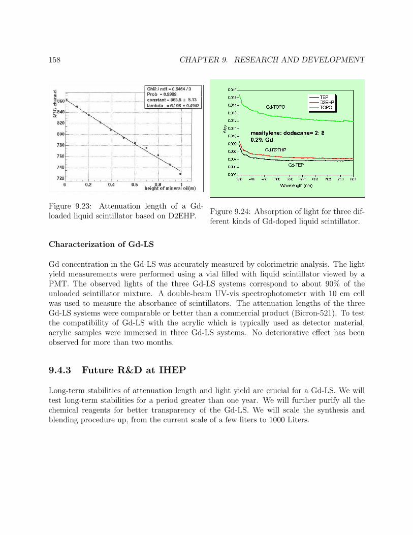
158 CHAPTER 9. RESEARCH AND DEVELOPMENT
Figure 9.23: Attenuation length of a Gd-loaded liquid scintillator based on D2EHP.
Figure 9.24: Absorption of light for three dif-ferent kinds of Gd-doped liquid scintillator.
Characterization of Gd-LS
Gd concentration in the Gd-LS was accurately measured by colorimetric analysis. The lightyield measurements were performed using a vial filled with liquid scintillator viewed by aPMT. The observed lights of the three Gd-LS systems correspond to about 90% of theunloaded scintillator mixture. A double-beam UV-vis spectrophotometer with 10 cm cellwas used to measure the absorbance of scintillators. The attenuation lengths of the threeGd-LS systems were comparable or better than a commercial product (Bicron-521). To testthe compatibility of Gd-LS with the acrylic which is typically used as detector material,acrylic samples were immersed in three Gd-LS systems. No deteriorative effect has beenobserved for more than two months.
9.4.3 Future R&D at IHEP
Long-term stabilities of attenuation length and light yield are crucial for a Gd-LS. We willtest long-term stabilities for a period greater than one year. We will further purify all thechemical reagents for better transparency of the Gd-LS. We will scale the synthesis andblending procedure up, from the current scale of a few liters to 1000 Liters.
Bibliography
[1] Preliminary feasibility study of the topography measurement of neutrino experiment(draft), IGG, Aug. 26, 2005.
[2] Preliminary feasibility study of the geological survey of the neutrino experiment, andthe references therein (draft), IGG, Aug. 26, 2005.
[3] Preliminary feasibility study of the physical survey of the neutrino experiment (draft),IGG, Aug. 26, 2005.
[4] For example, M. Robinson et al., Nucl. Instrumm. Methods A 511, 347 (2003); H. J. Kimet al., Astroparticle Physics 20, 549 (2004).
[5] R. Hertenberger et al., Phys. Rev. C 52, 3449 (1995).
[6] A. da Silva et al., Nucl. Instrum. Methods A 354, 553 (1995).
[7] Antonioli et al., Astroparticle Physics 7, 357 (1997); V. A. Kudryavtsev et al.,Phys. Lett. B 471, 251 (1999).
[8] http://pcfluka.mi.infn.it/
[9] http://theta13.phy.cuhk.edu.hk/
[10] GEANT4 - a simulation kit, Nucl. Instrum. Meth. A 506, 250 (2003);http://wwwasd.web.cern.ch/wwwasd/geant4/description.html
[11] T. K. Gaisser and T. Stanev, ’Cosmic Ray’, Review of Particle Physics, edited byL. Alvarez-Gaume et al., Phys. Lett. B 592, 228 (2004).
[12] A. Tang, M.-C. Chu, and K. B. Luk, ’Muon Transport Simulation for the NeutrinoExperiment at Daya Bay’, CUHK technical report, 2004 (unpublished).
[13] D. W. K. Ngai, M.-C. Chu, and K. B. Luk, ’Predicting Muon Spectrum at the AberdeenUnderground Lab’, CUHK technical report, 2005 (unpublished).
[14] Y. F. Wang et al., Phys. Rev. D 64, 013012 (2001).
159

160 BIBLIOGRAPHY

Chapter 10
Strategy and Organization
10.1 Run Plan
One advantage of using horizontal access tunnels is the ease of constructing several under-ground experimental halls at a relatively low cost. At Daya Bay, we can determine the valueof sin22θ13 using different combinations of the near, mid, and far sites. Since each configu-ration has different systematic issues, these combinations offer valuable internal consistencycheck.
Currently, we plan to utilize three configurations: near-mid, near-far, and mid-far, whichare described in the following sections.
10.1.1 Near-mid configuration
The deployment of the detectors will be completely dictated by the excavation of the tunnelsand construction of the underground experimental halls and the underground assembly roomfor filling the detector modules with liquid scintillator.
The detector modules will be first put together without the liquid scintillator in a centralassembly hall outside the tunnel while the access tunnel to the Daya Bay near site andthe construction tunnel to the mid site are being excavated. The total length of these twobranches of tunnels from the entrance portal to the mid site is less than one km. It isanticipated that their excavation will be completed in less than a year.
When the experimental halls and the underground assembly room at the Daya Bay nearsite and the mid site are ready, detector modules can be moved in for filling with liquidscintillator. To carry out the near-mid scheme, the completely assembled detector moduleswill then be installed at these two locations to determine sin22θ13 while the tunnels to theLing Ao near site and the far site are being constructed using the construction tunnel. In
161
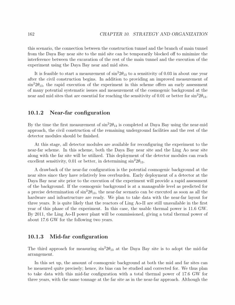
162 CHAPTER 10. STRATEGY AND ORGANIZATION
this scenario, the connection between the construction tunnel and the branch of main tunnelfrom the Daya Bay near site to the mid site can be temporarily blocked off to minimize theinterference between the excavation of the rest of the main tunnel and the execution of theexperiment using the Daya Bay near and mid sites.
It is feasible to start a measurement of sin22θ13 to a sensitivity of 0.03 in about one yearafter the civil construction begins. In addition to providing an improved measurement ofsin22θ13, the rapid execution of the experiment in this scheme offers an early assessmentof many potential systematic issues and measurement of the cosmogenic background at thenear and mid sites that are essential for reaching the sensitivity of 0.01 or better for sin22θ13.
10.1.2 Near-far configuration
By the time the first measurement of sin22θ13 is completed at Daya Bay using the near-midapproach, the civil construction of the remaining underground facilities and the rest of thedetector modules should be finished.
At this stage, all detector modules are available for reconfiguring the experiment to thenear-far scheme. In this scheme, both the Daya Bay near site and the Ling Ao near sitealong with the far site will be utilized. This deployment of the detector modules can reachexcellent sensitivity, 0.01 or better, in determining sin22θ13.
A drawback of the near-far configuration is the potential cosmogenic background at thenear sites since they have relatively less overburden. Early deployment of a detector at theDaya Bay near site prior to the execution of the experiment will provide a rapid assessmentof the background. If the cosmogenic background is at a manageable level as predicted fora precise determination of sin22θ13, the near-far scenario can be executed as soon as all thehardware and infrastructure are ready. We plan to take data with the near-far layout forthree years. It is quite likely that the reactors of Ling Ao-II are still unavailable in the firstyear of this phase of the experiment. In this case, the usable thermal power is 11.6 GW.By 2011, the Ling Ao-II power plant will be commissioned, giving a total thermal power ofabout 17.6 GW for the following two years.
10.1.3 Mid-far configuration
The third approach for measuring sin22θ13 at the Daya Bay site is to adopt the mid-fararrangement.
In this set up, the amount of cosmogenic background at both the mid and far sites canbe measured quite precisely; hence, its bias can be studied and corrected for. We thus planto take data with this mid-far configuration with a total thermal power of 17.6 GW forthree years, with the same tonnage at the far site as in the near-far approach. Although the
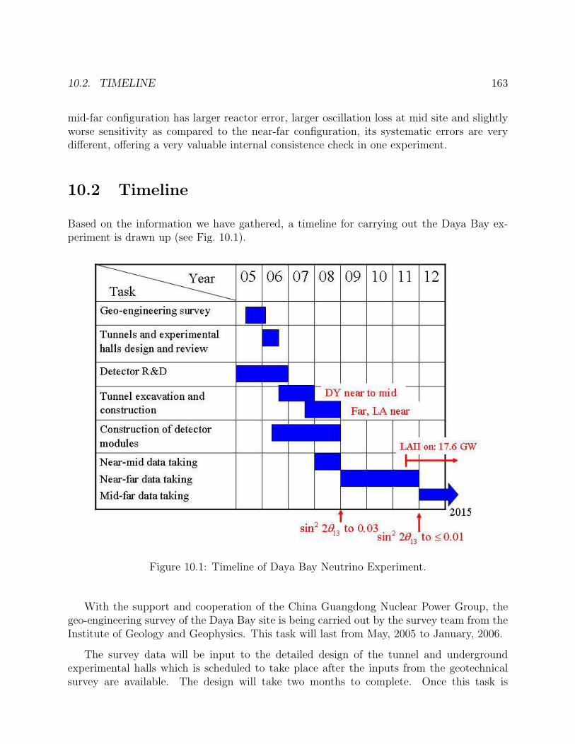
10.2. TIMELINE 163
mid-far configuration has larger reactor error, larger oscillation loss at mid site and slightlyworse sensitivity as compared to the near-far configuration, its systematic errors are verydifferent, offering a very valuable internal consistence check in one experiment.
10.2 Timeline
Based on the information we have gathered, a timeline for carrying out the Daya Bay ex-periment is drawn up (see Fig. 10.1).
Figure 10.1: Timeline of Daya Bay Neutrino Experiment.
With the support and cooperation of the China Guangdong Nuclear Power Group, thegeo-engineering survey of the Daya Bay site is being carried out by the survey team from theInstitute of Geology and Geophysics. This task will last from May, 2005 to January, 2006.
The survey data will be input to the detailed design of the tunnel and undergroundexperimental halls which is scheduled to take place after the inputs from the geotechnicalsurvey are available. The design will take two months to complete. Once this task is
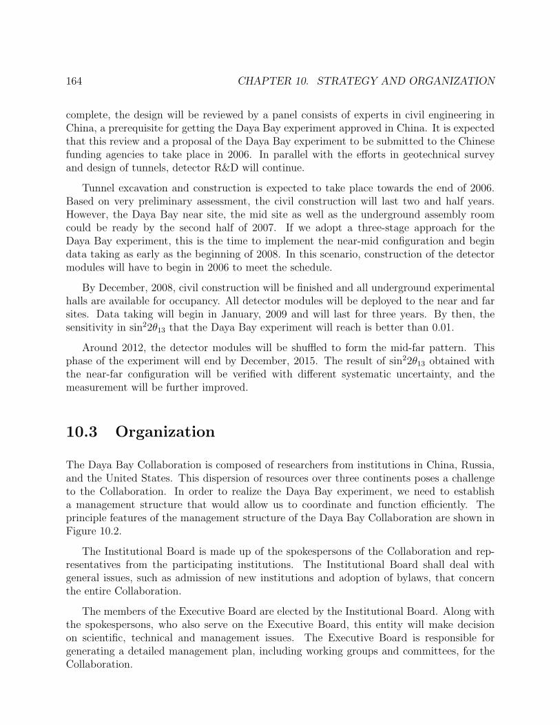
164 CHAPTER 10. STRATEGY AND ORGANIZATION
complete, the design will be reviewed by a panel consists of experts in civil engineering inChina, a prerequisite for getting the Daya Bay experiment approved in China. It is expectedthat this review and a proposal of the Daya Bay experiment to be submitted to the Chinesefunding agencies to take place in 2006. In parallel with the efforts in geotechnical surveyand design of tunnels, detector R&D will continue.
Tunnel excavation and construction is expected to take place towards the end of 2006.Based on very preliminary assessment, the civil construction will last two and half years.However, the Daya Bay near site, the mid site as well as the underground assembly roomcould be ready by the second half of 2007. If we adopt a three-stage approach for theDaya Bay experiment, this is the time to implement the near-mid configuration and begindata taking as early as the beginning of 2008. In this scenario, construction of the detectormodules will have to begin in 2006 to meet the schedule.
By December, 2008, civil construction will be finished and all underground experimentalhalls are available for occupancy. All detector modules will be deployed to the near and farsites. Data taking will begin in January, 2009 and will last for three years. By then, thesensitivity in sin22θ13 that the Daya Bay experiment will reach is better than 0.01.
Around 2012, the detector modules will be shuffled to form the mid-far pattern. Thisphase of the experiment will end by December, 2015. The result of sin22θ13 obtained withthe near-far configuration will be verified with different systematic uncertainty, and themeasurement will be further improved.
10.3 Organization
The Daya Bay Collaboration is composed of researchers from institutions in China, Russia,and the United States. This dispersion of resources over three continents poses a challengeto the Collaboration. In order to realize the Daya Bay experiment, we need to establisha management structure that would allow us to coordinate and function efficiently. Theprinciple features of the management structure of the Daya Bay Collaboration are shown inFigure 10.2.
The Institutional Board is made up of the spokespersons of the Collaboration and rep-resentatives from the participating institutions. The Institutional Board shall deal withgeneral issues, such as admission of new institutions and adoption of bylaws, that concernthe entire Collaboration.
The members of the Executive Board are elected by the Institutional Board. Along withthe spokespersons, who also serve on the Executive Board, this entity will make decisionon scientific, technical and management issues. The Executive Board is responsible forgenerating a detailed management plan, including working groups and committees, for theCollaboration.
10.3. ORGANIZATION 165
Figure 10.2: Management structure of the Daya Bay Collaboration.
The spokespersons are responsible for the daily operation of the Collaboration. Theyalso represent the Collaboration’s interests in the community, in the laboratory and to thefunding agencies.
The group leaders, appointed by the Executive Board, are responsible for planning andorganizing the group activities to ensure the technical requirements, cost, and schedule aremet.
During the design and construction phases there will be project managers, appointed bythe Executive Board, to oversee the technical aspect of the experiment. The project managerswill plan, organize, review, and monitor the progress of all subsystems. In addition, theproject managers will handle budget management, allocation of budgets, and preparation aswell as submission of project progress reports for the Collaboration.

166 CHAPTER 10. STRATEGY AND ORGANIZATION
Appendix A
Past Reactor Neutrino Experiments
The detectors of the early reactor neutrino experiments, for example ILL [1], Gosgen [2],and Bugey [3], were located very close to the reactor (up to 100 m), and they were thussensitive to ∆m2
31 of the order of 5× 10⁻² eV2 which is about twenty times larger than thecurrent best-fit value where the oscillation related to the mixing angle θ31 is expected totake place. In the nineties, motivated by the observation of atmospheric neutrino oscillation,two reactor-based neutrino experiments, Chooz [4] and Palo Verde [5], were carried out toinvestigate this surprising phenomenon. Based on ∆m2
32 = 1.5 × 10⁻² eV2 as reported byKamiokande [6], the baselines of Chooz and Palo Verde were chosen to be about 1 km,corresponding to the location of the first oscillation maximum of νe → νµ when probed withlow-energy reactor νe. Since the νµ coming from oscillation does not have enough energy toproduce a µ+ through the charged-current process, reactor-based neutrino experiments aredisappearance experiments. Both Chooz and Palo Verde were looking for a deficit in theνe flux at the location of the detector, as compared with the calculated flux assuming nooscillation occurred. With only one detector, both experiments must rely on the operationalinformation of the reactors, in particular, the composition of the nuclear fuel and the amountof thermal power generated as a function of time, for calculating the rate of νe produced inthe fission processes.
Chooz and Palo Verde utilized Gd-doped liquid scintillator to detect the reactor νe viathe inverse beta-decay νep → ne+ reaction. The ionization loss and subsequent annihilationof the positron give rise to a fast signal obtained with an array of photo-multiplier tubes.The energy associated with this signal is termed the prompt energy, Ep. ¿From kinematicconsideration, it is easy to realize that Ep is directly related to the energy of the incident νe.After random walking for about 30 µs, the neutron is captured by a Gd nucleus, emittingseveral gamma-ray photons with a total energy of about 8 MeV. This signal is called thedelayed energy, Ed. The temporal and spatial correlation between the prompt energy andthe delayed energy constitutes a powerful tool for identifying the νe and for suppressingbackgrounds.
167
168 APPENDIX A. PAST REACTOR NEUTRINO EXPERIMENTS
Both Chooz and Palo Verde did not observe any rate deficit in νe. This null result isused to set a limit in the neutrino mixing angle θ13. In terms of sin22θ13, Chooz obtainedthe best limit of 0.2 at the 90% confidence level.
KamLAND [7] is the only reactor-based neutrino experiment currently taking data. It isdesigned to address the question of neutrino oscillation first discovered as a deficit in the solar-neutrino flux on Earth. Through a series of studies of solar neutrinos, there is compellingevidence that the mass-squared difference, ∆m2
21, should be less than 10−4 eV2. In order toinvestigate this phenomenon with anti-neutrinos from nuclear reactors, the baseline has tobe on the order of a hundred km and the detector be about a kilo-ton in mass. These arethe unique features of KamLAND. Recently, KamLAND has observed a reduction in anti-neutrino flux, which strengthens the evidence of neutrino oscillation and favors the largemixing-angle (LMA) solution.
In the following sections, some of the features of Gosgen, Bugey, Chooz, Palo Verde andKamLAND that are relevant to the design of the next generation of reactor-based neutrinoexperiments for determining θ13 are summarized.
A.1 Gosgen
The Gosgen experiment was conducted at the 2.8 GWth nuclear power reactor at Gosgen(Switzerland). The energy spectrum of the anti-neutrinos was measured at three distances,37.9, 45.9, and 64.7 m, from the reactor core. The experiment was carried out during 3periods from 1981 to 1985. Roughly 104 anti-neutrinos were registered at each of the threepositions.
The detector is approximately one cubic meter in size and consists of two different kindsof detector systems sandwiching each other as shown in Fig. A.1. The detector elementsrecord, respectively, the positrons and neutrons generated in the inverse β-decay reactionsνe +p → e++n. One system is made of thirty cells filled with a proton-rich liquid scintillatorand arranged in five planes served both as the target for the incident anti-neutrinos and asdetector for sensing the generated positrons. The neutrons emerging with an energy ofseveral keV are thermalized in the scintillator cell within a few µs and diffuse within a meandiffusion time of about 150 µs into one of the adjacent wire chambers filled with 3He, wherethey are detected. An anti-neutrino candidate satisfies a proper spatial correlation as wellas a coincidence within a time window of 20 µs between a positron in a scintillator cell anda neutron in one of the multiwire proportional chambers.
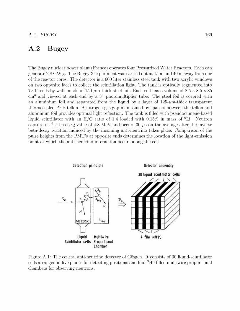
A.2. BUGEY 169
A.2 Bugey
The Bugey nuclear power plant (France) operates four Pressurized Water Reactors. Each cangenerate 2.8 GWth. The Bugey-3 experiment was carried out at 15 m and 40 m away from oneof the reactor cores. The detector is a 600 liter stainless steel tank with two acrylic windowson two opposite faces to collect the scintillation light. The tank is optically segmented into7×14 cells by walls made of 150-µm-thick steel foil. Each cell has a volume of 8.5× 8.5× 85cm3 and viewed at each end by a 3” photomultiplier tube. The steel foil is covered withan aluminium foil and separated from the liquid by a layer of 125-µm-thick transparentthermosealed PEP teflon. A nitrogen gas gap maintained by spacers between the teflon andaluminium foil provides optimal light reflection. The tank is filled with pseudocumene-basedliquid scintillator with an H/C ratio of 1.4 loaded with 0.15% in mass of 6Li. Neutroncapture on 6Li has a Q-value of 4.8 MeV and occurs 30 µs on the average after the inversebeta-decay reaction induced by the incoming anti-neutrino takes place. Comparison of thepulse heights from the PMT’s at opposite ends determines the location of the light-emissionpoint at which the anti-neutrino interaction occurs along the cell.
Figure A.1: The central anti-neutrino detector of Gosgen. It consists of 30 liquid-scintillatorcells arranged in five planes for detecting positrons and four 3He-filled multiwire proportionalchambers for observing neutrons.
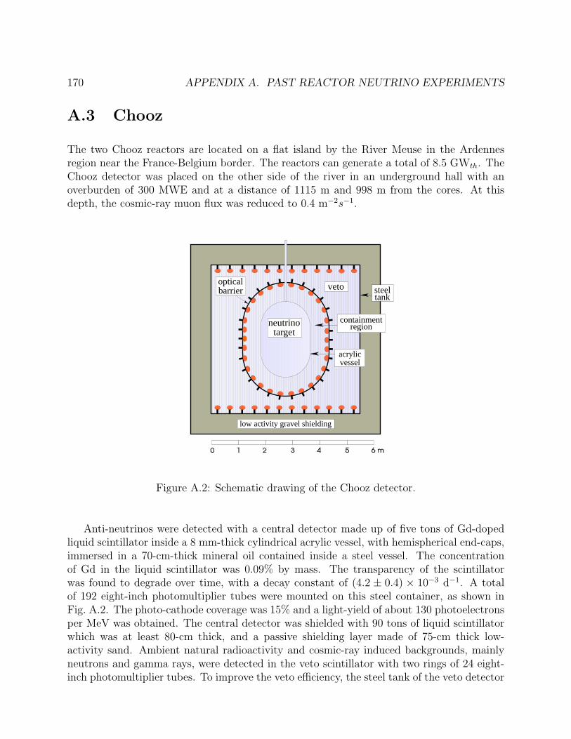
170 APPENDIX A. PAST REACTOR NEUTRINO EXPERIMENTS
A.3 Chooz
The two Chooz reactors are located on a flat island by the River Meuse in the Ardennesregion near the France-Belgium border. The reactors can generate a total of 8.5 GWth. TheChooz detector was placed on the other side of the river in an underground hall with anoverburden of 300 MWE and at a distance of 1115 m and 998 m from the cores. At thisdepth, the cosmic-ray muon flux was reduced to 0.4 m−2s−1.
veto
acrylicvessel
neutrinotarget
opticalbarrier
low activity gravel shielding
containmentregion
steeltank
Figure A.2: Schematic drawing of the Chooz detector.
Anti-neutrinos were detected with a central detector made up of five tons of Gd-dopedliquid scintillator inside a 8 mm-thick cylindrical acrylic vessel, with hemispherical end-caps,immersed in a 70-cm-thick mineral oil contained inside a steel vessel. The concentrationof Gd in the liquid scintillator was 0.09% by mass. The transparency of the scintillatorwas found to degrade over time, with a decay constant of (4.2 ± 0.4) × 10−3 d−1. A totalof 192 eight-inch photomultiplier tubes were mounted on this steel container, as shown inFig. A.2. The photo-cathode coverage was 15% and a light-yield of about 130 photoelectronsper MeV was obtained. The central detector was shielded with 90 tons of liquid scintillatorwhich was at least 80-cm thick, and a passive shielding layer made of 75-cm thick low-activity sand. Ambient natural radioactivity and cosmic-ray induced backgrounds, mainlyneutrons and gamma rays, were detected in the veto scintillator with two rings of 24 eight-inch photomultiplier tubes. To improve the veto efficiency, the steel tank of the veto detector
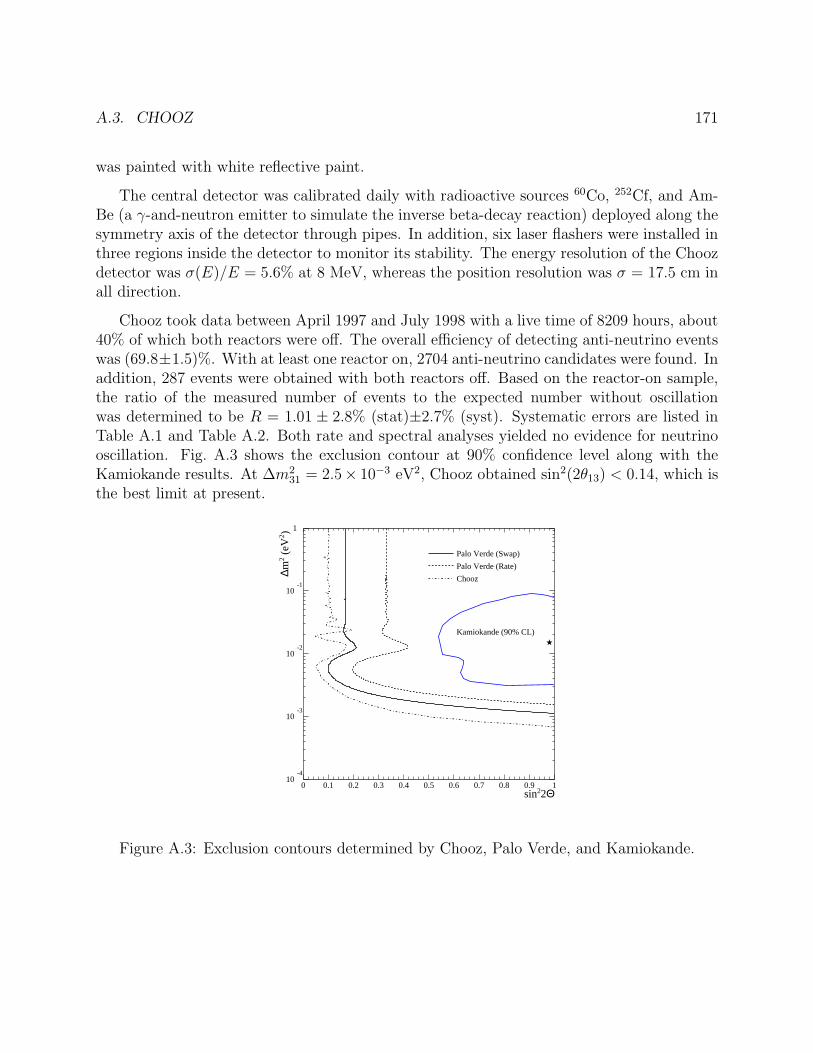
A.3. CHOOZ 171
was painted with white reflective paint.
The central detector was calibrated daily with radioactive sources 60Co, 252Cf, and Am-Be (a γ-and-neutron emitter to simulate the inverse beta-decay reaction) deployed along thesymmetry axis of the detector through pipes. In addition, six laser flashers were installed inthree regions inside the detector to monitor its stability. The energy resolution of the Choozdetector was σ(E)/E = 5.6% at 8 MeV, whereas the position resolution was σ = 17.5 cm inall direction.
Chooz took data between April 1997 and July 1998 with a live time of 8209 hours, about40% of which both reactors were off. The overall efficiency of detecting anti-neutrino eventswas (69.8±1.5)%. With at least one reactor on, 2704 anti-neutrino candidates were found. Inaddition, 287 events were obtained with both reactors off. Based on the reactor-on sample,the ratio of the measured number of events to the expected number without oscillationwas determined to be R = 1.01 ± 2.8% (stat)±2.7% (syst). Systematic errors are listed inTable A.1 and Table A.2. Both rate and spectral analyses yielded no evidence for neutrinooscillation. Fig. A.3 shows the exclusion contour at 90% confidence level along with theKamiokande results. At ∆m2
31 = 2.5× 10⁻³ eV2, Chooz obtained sin2(2θ13) < 0.14, which isthe best limit at present.
10-4
10-3
10-2
10-1
1
0 0.1 0.2 0.3 0.4 0.5 0.6 0.7 0.8 0.9 1sin22Θ
∆m2 (
eV2 )
Kamiokande (90% CL)
Palo Verde (Swap)
Palo Verde (Rate)
Chooz
Figure A.3: Exclusion contours determined by Chooz, Palo Verde, and Kamiokande.
172 APPENDIX A. PAST REACTOR NEUTRINO EXPERIMENTS
parameter relative error (%)
reaction cross section 1.9number of protons 0.8detection efficiency 1.5reactor power 0.7energy released per fission 0.6combined 2.7
Table A.1: Contributions to the overall systematic uncertainty in the absolute normalization.
selection ε (%) relative error (%)
positron energy 97.8 0.8positron-geode distance 99.9 0.1neutron capture 84.6 1.0capture energy containment 94.6 0.4neutron-geode distance 99.5 0.1neutron delay 93.7 0.4positron-neutron distance 98.4 0.3neutron multiplicity 97.4 0.5combined 69.8 1.5
Table A.2: Summary of the anti-neutrino detection efficiency.
A.4 Palo Verde
The Palo Verde experiment utilized the Palo Verde Nuclear Generating Station, which isabout 70 km west of Phoenix, Arizona. The detector was located underground with 32 m ofoverburden, reducing the cosmic-ray muon flux to 22 m−2 s−1 but about 50 times higher thanthat at Chooz. The detector was 890 m from the outer reactors and 750 m from the core atthe center. The three identical reactors generated a total of 11.63 GW thermal power. Thewalls of the hall were made of crushed marble with low natural radioactivity, reducing theambient gamma ray by a factor of ten.
Fig. A.4 is a sketch of the Palo Verde detector. The 11.34 tons of Gd-loaded liquidscintillator was contained in a 6 by 11 array of acrylic cells. Each cell was 9-m long, 12.7-cmwide and 25.4-cm tall. Between the liquid scintillator and the photomultiplier tube at eachend of a cell, a 0.8-m long region was filled with mineral oil that blocked external gamma rayand neutron backgrounds from entering the fiducial region. The array was further shieldedat all sides with 1-m thick of purified water in steel tanks. Outside the water jacket wasan array of muon veto-counters made of PVC tanks filled with dilute liquid scintillator andviewed with photomultiplier tubes at both ends. Contrary to the Chooz detector, signals
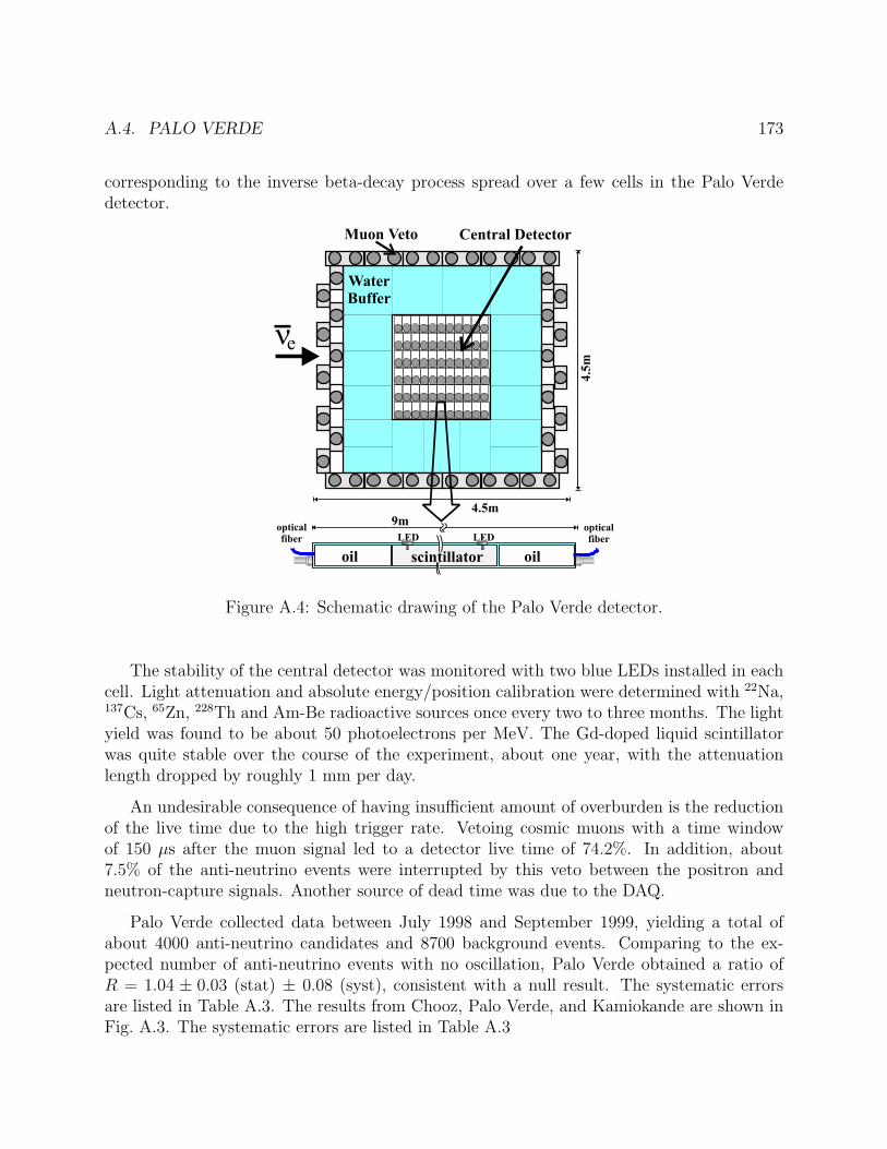
A.4. PALO VERDE 173
corresponding to the inverse beta-decay process spread over a few cells in the Palo Verdedetector.
Figure A.4: Schematic drawing of the Palo Verde detector.
The stability of the central detector was monitored with two blue LEDs installed in eachcell. Light attenuation and absolute energy/position calibration were determined with 22Na,137Cs, 65Zn, 228Th and Am-Be radioactive sources once every two to three months. The lightyield was found to be about 50 photoelectrons per MeV. The Gd-doped liquid scintillatorwas quite stable over the course of the experiment, about one year, with the attenuationlength dropped by roughly 1 mm per day.
An undesirable consequence of having insufficient amount of overburden is the reductionof the live time due to the high trigger rate. Vetoing cosmic muons with a time windowof 150 µs after the muon signal led to a detector live time of 74.2%. In addition, about7.5% of the anti-neutrino events were interrupted by this veto between the positron andneutron-capture signals. Another source of dead time was due to the DAQ.
Palo Verde collected data between July 1998 and September 1999, yielding a total ofabout 4000 anti-neutrino candidates and 8700 background events. Comparing to the ex-pected number of anti-neutrino events with no oscillation, Palo Verde obtained a ratio ofR = 1.04 ± 0.03 (stat) ± 0.08 (syst), consistent with a null result. The systematic errorsare listed in Table A.3. The results from Chooz, Palo Verde, and Kamiokande are shown inFig. A.3. The systematic errors are listed in Table A.3
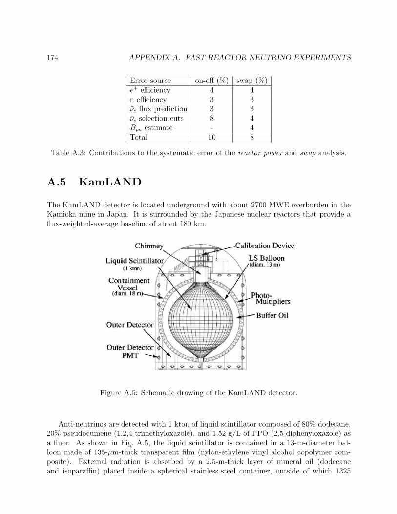
174 APPENDIX A. PAST REACTOR NEUTRINO EXPERIMENTS
Error source on-off (%) swap (%)e+ efficiency 4 4n efficiency 3 3νe flux prediction 3 3νe selection cuts 8 4Bpn estimate - 4Total 10 8
Table A.3: Contributions to the systematic error of the reactor power and swap analysis.
A.5 KamLAND
The KamLAND detector is located underground with about 2700 MWE overburden in theKamioka mine in Japan. It is surrounded by the Japanese nuclear reactors that provide aflux-weighted-average baseline of about 180 km.
Figure A.5: Schematic drawing of the KamLAND detector.
Anti-neutrinos are detected with 1 kton of liquid scintillator composed of 80% dodecane,20% pseudocumene (1,2,4-trimethyloxazole), and 1.52 g/L of PPO (2,5-diphenyloxazole) asa fluor. As shown in Fig. A.5, the liquid scintillator is contained in a 13-m-diameter bal-loon made of 135-µm-thick transparent film (nylon-ethylene vinyl alcohol copolymer com-posite). External radiation is absorbed by a 2.5-m-thick layer of mineral oil (dodecaneand isoparaffin) placed inside a spherical stainless-steel container, outside of which 1325
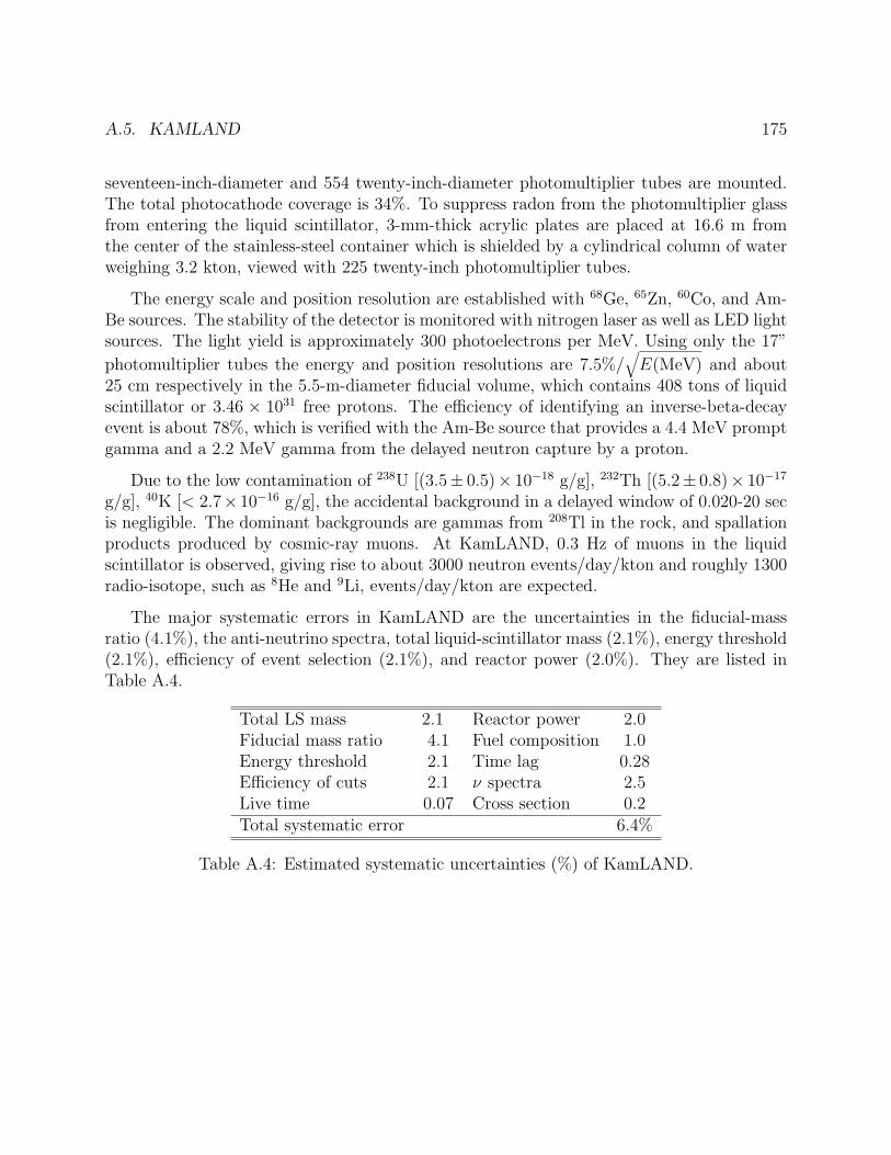
A.5. KAMLAND 175
seventeen-inch-diameter and 554 twenty-inch-diameter photomultiplier tubes are mounted.The total photocathode coverage is 34%. To suppress radon from the photomultiplier glassfrom entering the liquid scintillator, 3-mm-thick acrylic plates are placed at 16.6 m fromthe center of the stainless-steel container which is shielded by a cylindrical column of waterweighing 3.2 kton, viewed with 225 twenty-inch photomultiplier tubes.
The energy scale and position resolution are established with 68Ge, 65Zn, 60Co, and Am-Be sources. The stability of the detector is monitored with nitrogen laser as well as LED lightsources. The light yield is approximately 300 photoelectrons per MeV. Using only the 17”
photomultiplier tubes the energy and position resolutions are 7.5%/√
E(MeV) and about25 cm respectively in the 5.5-m-diameter fiducial volume, which contains 408 tons of liquidscintillator or 3.46 × 1031 free protons. The efficiency of identifying an inverse-beta-decayevent is about 78%, which is verified with the Am-Be source that provides a 4.4 MeV promptgamma and a 2.2 MeV gamma from the delayed neutron capture by a proton.
Due to the low contamination of 238U [(3.5± 0.5)× 10−18 g/g], 232Th [(5.2± 0.8)× 10−17
g/g], 40K [< 2.7× 10⁻¹⁶ g/g], the accidental background in a delayed window of 0.020-20 secis negligible. The dominant backgrounds are gammas from 208Tl in the rock, and spallationproducts produced by cosmic-ray muons. At KamLAND, 0.3 Hz of muons in the liquidscintillator is observed, giving rise to about 3000 neutron events/day/kton and roughly 1300radio-isotope, such as 8He and 9Li, events/day/kton are expected.
The major systematic errors in KamLAND are the uncertainties in the fiducial-massratio (4.1%), the anti-neutrino spectra, total liquid-scintillator mass (2.1%), energy threshold(2.1%), efficiency of event selection (2.1%), and reactor power (2.0%). They are listed inTable A.4.
Total LS mass 2.1 Reactor power 2.0Fiducial mass ratio 4.1 Fuel composition 1.0Energy threshold 2.1 Time lag 0.28Efficiency of cuts 2.1 ν spectra 2.5Live time 0.07 Cross section 0.2Total systematic error 6.4%
Table A.4: Estimated systematic uncertainties (%) of KamLAND.

Bibliography
[1] H. Kwon et al., Phys. Rev. D24, 1097 (1981).
[2] G. Zacek et al., Phys. Rev. D34, 2621 (1986).
[3] Y. Declais et al., Phys. Lett. B338, 383 (1994). B. Ackar et al., Nucl. Phys. B434, 503(1995); B. Ackar et al., Phys. Lett. B374, 243 (1996).
[4] M. Apollonio et al., Eur. Phys. J. C27, 331 (2003).
[5] F. Boehm et al., Phys. Rev. D62, 072002 (2000).
[6] K. S. Hirata et al., Phys. Lett. B205, 416 (1988); Y. Fukuda et al., Phys. Lett. B335,237 (1994).
[7] K. Eguchi et al., Phys. Rev. Lett. 90, 021802 (2003).
176
List of Figures
2.1 Oscillation parameters in two-flavor mixing approximation. . . . . . . . . . . 7
2.2 Oscillation parameters in two-flavor mixing approximation. . . . . . . . . . . 7
2.3 Normal and inverted spectra: normal ∆m232 > 0; inverted ∆m2
32 < 0. . . . . . 9
2.4 Level structures of four neutrinos. The 2+2 scenario is disfavored comparedto the 3+1 scenario, but neither provides a good fit to the data. . . . . . . . 9
2.5 The ∆χ2 as a function of sin2 θ13 obtained respectively by BGP (left) in Ref.[31] and MSTV (right) in Ref. [32]. . . . . . . . . . . . . . . . . . . . . . . . 12
2.6 P0: the slowly rising and falling curve, Pdis: the oscillating curve around P0,and Pnet: the low value oscillating curve. The various parameters used aredescribed in the text. . . . . . . . . . . . . . . . . . . . . . . . . . . . . . . . 18
2.7 Integrated Pnet as a function of the baseline Lfar. The three curves covers the90% CL range in ∆m2
32 [3]. . . . . . . . . . . . . . . . . . . . . . . . . . . . . 20
2.8 Size of Pdis, P0, Pnet, and P2, integrated over neutrino energy spectrum, versusbaseline for sin2 2θ13 = 0.02. . . . . . . . . . . . . . . . . . . . . . . . . . . . 20
3.1 Fission rate of each isotope as a function of time from a Monte Carlo simula-tion [7]. . . . . . . . . . . . . . . . . . . . . . . . . . . . . . . . . . . . . . . 31
3.2 Yield of antineutrinos per fission for the listed isotopes. These are determinedby converting the corresponding measured β spectra [9]. . . . . . . . . . . . 32
3.3 Antineutrino energy spectrum for four isotopes following the parametrizationof Vogel and Engel [10]. . . . . . . . . . . . . . . . . . . . . . . . . . . . . . 32
3.4 Total cross section of the inverse beta decay calculated in leading order andnext-to-leading order. . . . . . . . . . . . . . . . . . . . . . . . . . . . . . . . 33
3.5 Recoil neutron energy spectrum from inverse beta decay weighted by the an-tineutrino energy spectrum. . . . . . . . . . . . . . . . . . . . . . . . . . . . 34
177
178 LIST OF FIGURES
3.6 Angular distributions of the positrons and recoil neutrons in the laboratoryframe. . . . . . . . . . . . . . . . . . . . . . . . . . . . . . . . . . . . . . . . 34
3.7 Predicted antineutrino event rate of the Palo Verde experiment as a functionof time with the reactor power, fission rate and inverse beta decay cross sectiontaken into account. . . . . . . . . . . . . . . . . . . . . . . . . . . . . . . . . 35
3.8 Antineutrino energy spectrum, total cross section of inverse beta decay, andcount rate as a function of the antineutrino energy. . . . . . . . . . . . . . . 35
4.1 Daya Bay and the vicinity. The nuclear power plants are located on the southshore of the west to east going Minor Daya Peninsula as marked. A towncalled Dapeng is located in the southwest of the peninsula. . . . . . . . . . . 38
4.2 Monthly average temperature from Sep., 1984 to Aug., 1986 from data pro-vided by the Da Ken weather station. The horizontal axis gives the monthsfrom January to December and the vertical axis is the average temperaturein centigrade. . . . . . . . . . . . . . . . . . . . . . . . . . . . . . . . . . . . 41
4.3 Monthly average rainfall from 1983 to 1992 from data provided by the DaKen weather station. The horizontal axis gives the months from January toDecember and the vertical axis is the amount of rainfall in mm. . . . . . . . 41
4.4 Layout of the Daya Bay-Ling Ao reactor cores, the future Ling Ao-II cores(also known as Ling Dong), and possible detector sites. The green lines rep-resent access tunnels, and blue lines are main tunnels connecting the under-ground detector halls. . . . . . . . . . . . . . . . . . . . . . . . . . . . . . . . 44
4.5 Cross section of the access and main tunnels. . . . . . . . . . . . . . . . . . . 46
5.1 Cross section of a detector module showing the three-layer structure. . . . . 50
5.2 Sensitivity of sin22θ13 at 90% C.L. as a function of target mass at the far site. 51
5.3 Layout of the antineutrino detector used in the GEANT3 simulation. Theouter-most layer is rock around the underground lab. Four detector modulesare shielded by 2-m-thick water buffer (layer in blue). The three-layer struc-ture of module is shown in white (oil), light blue (gamma catcher), and yellow(target). . . . . . . . . . . . . . . . . . . . . . . . . . . . . . . . . . . . . . . 52
5.4 The emitted gamma spectrum of Gd after neutron capture. . . . . . . . . . . 53
5.5 Effect of scintillation light quenching in proton-recoil events from the Am-Besource. Accurate simulation of proton recoil is useful for understanding theantineutrino backgrounds resulting from fast neutrons. . . . . . . . . . . . . 53
LIST OF FIGURES 179
5.6 Variation of attenuation length of one cell (top) and all cells(bottom) for threeyears of operation at Palo Verde. . . . . . . . . . . . . . . . . . . . . . . . . 55
5.7 Light yield of all batches of BC521. . . . . . . . . . . . . . . . . . . . . . . . 55
5.8 Longitudinal section of a detector module showing the acrylic vessels holdingthe Gd-doped liquid scintillator at the center, and liquid scintillator betweenthe acrylic containers. The PMTs are mounted inside the outer-most stainlesssteel tank. . . . . . . . . . . . . . . . . . . . . . . . . . . . . . . . . . . . . . 57
5.9 The vertex reconstruction resolution, determined by a maximum likelihood fit,for a point-like 8 MeV event. The x-axis is the residual of the reconstructedvertex from the true vertex and the y-axis is the number of events per bin. . 58
5.10 Efficiency of the 6-MeV energy cut as a function of the gamma-catcher thickness. 59
5.11 Total number of observed photoelectrons (chqtot) versus vertex position inequal-volume bin (eqvcyl) for 1-MeV gamma rays. The center of the detectoris at eqvcyl = 0, and the wall of the container is at eqvcyl = 40000. . . . . . 61
5.12 Number of fast neutrons per day for a 20-t module at the far site of Daya Bayas a function of the thickness of water buffer. . . . . . . . . . . . . . . . . . . 63
5.13 A conceptual design of the water buffer using a cylindrical tank. The topcovers are pulled open to show the detector modules submerged in water.Muon tracking detectors are mounted on the outside and the top of the tank. 64
5.14 Stress (left panel) and deformation (right panel) of the cylindrical water tankdetermined by finite-element analysis. . . . . . . . . . . . . . . . . . . . . . . 65
5.15 Conceptual design of the water pool. . . . . . . . . . . . . . . . . . . . . . . 66
5.16 Veto detector modules are mounted on the stainless steel bars along the wallsand the bottom of the water pool. Special reinforcement is needed on the topside to support the veto modules. . . . . . . . . . . . . . . . . . . . . . . . . 66
5.17 Sketch of a Resistive Plate Chamber. . . . . . . . . . . . . . . . . . . . . . . 67
5.18 Efficiency of the BESIII RPC versus high voltage for different thresholds. . . 68
5.19 Noise rate of the BESIII RPC versus high voltage for different thresholds. . . 68
5.20 A plastic-scintillator module of scintillator strips during assembly. . . . . . . 69
5.21 Layout of the electronics in the endcap of the module. A Front-End Cardplugged to the Hamamatsu H7546 PMT as well as the DAQ card is shown. . 70
5.22 Response to minimum ionizing particles measured by left PMT (red points)and right PMT (green points) for a scintillator strip used in OPERA. . . . . 70
5.23 Block diagram of a readout module for processing PMT signals . . . . . . . 73
180 LIST OF FIGURES
5.24 Block diagram of a front-end readout module for processing the RPC signals. 75
5.25 A simplified trigger scheme . . . . . . . . . . . . . . . . . . . . . . . . . . . . 76
6.1 Three dimensional profile of Pai Ya Mountain generated from a 1:5000 topo-graphic map of the Daya Bay site. . . . . . . . . . . . . . . . . . . . . . . . . 85
6.2 Comparison of the modified formula (solid lines) with data. Calculations withthe standard Gaisser’s formula are shown in dashed lines. The data is takenfrom Ref. [4, 5]. . . . . . . . . . . . . . . . . . . . . . . . . . . . . . . . . . . 86
6.3 Muon flux as a function of the energy of the surviving muons. The upper,middle, and lower curves are the muon fluxes for the DYB near site, the LAnear site, and the far site, respectively. . . . . . . . . . . . . . . . . . . . . . 87
6.4 Neutron yield as a function of mean muon energy. The stars indicate FLUKAsimulation results. The solid line is a fit of the simulation results to a power lawin Eq. 6.3. The crosses are data points taken from underground experimentsat various depths. For details see Ref. [6]. . . . . . . . . . . . . . . . . . . . . 89
6.5 Comparison of measured neutron energy spectrum with the empirical functionin Eq. 6.4. . . . . . . . . . . . . . . . . . . . . . . . . . . . . . . . . . . . . . 89
6.6 The prompt energy spectrum of fast neutron backgrounds at the Daya Bayfar detector. The inset is an expanded view of the spectrum from 1 to 10 MeV. 90
6.7 Fitting results as a function of the muon rate. The error bars show theprecision of the fitting. The χ2 fitting uses the same muon rate as ML fittingbut shown on the right of it. . . . . . . . . . . . . . . . . . . . . . . . . . . . 93
6.8 The fitting precision as a function of the muon rate, comparing with theanalytic estimation of Eq. 6.9. The y-axis shows the relative resolution of thebackground-to-signal ratio. . . . . . . . . . . . . . . . . . . . . . . . . . . . . 93
6.9 Spectrum of natural radioactivity measured with a Ge crystal in the HongKong Aberdeen Tunnel. . . . . . . . . . . . . . . . . . . . . . . . . . . . . . 95
6.10 Spectra of three major backgrounds for the Daya Bay experiment and theirsize relative to the oscillation signal. . . . . . . . . . . . . . . . . . . . . . . 97
7.1 Layout of the Daya Bay experiment. . . . . . . . . . . . . . . . . . . . . . . 103
7.2 Spectra of prompt energy for true energy, simulated energy (Geant Energy),and reconstructed energy at around 1 MeV. The full spectrum is shown inthe inset, where the red line corresponds to the true energy and the black onecorresponds to the reconstructed energy. . . . . . . . . . . . . . . . . . . . . 107
LIST OF FIGURES 181
7.3 Neutron energy distribution for neutrino events in a 20-ton detector modulewith 45 cm gamma catcher. The energy of neutron capture on Gd is simulatedby Geant3, followed by energy reconstruction. . . . . . . . . . . . . . . . . . 108
7.4 Neutron versus positron energy for neutrino-like events at Chooz [1]. Theevents in area D have delayed energy 4 - 6 MeV due to intrinsic radioactivityin liquid scintillator and acrylic vessel. . . . . . . . . . . . . . . . . . . . . . 108
7.5 Monte Carlo simulation of neutron capture time with 0.1% Gd concentrationin liquid scintillator. The upper plot shows the inefficiency of ending time cutand the lower plot shows the same for starting time cut. . . . . . . . . . . . 109
7.6 Sensitivity limit of sin2 2θ13 as a function of the baseline for three ∆m231 values.117
7.7 Muon flux in the vicinity of the far site. The blue lines shows the contourof the mountain and the red dots are the grid points that the calculation iscarried on. . . . . . . . . . . . . . . . . . . . . . . . . . . . . . . . . . . . . . 118
7.8 Site optimization using the global χ2 analysis. The optimal sites are labelledwith red triangles. The stars show the reactors. The contours show thesensitivity when one site varies and the other two are fixed at optimal sites.The red line with ticks are the perpendicular bisectors of reactor pairs. Themountain contours are also shown as background of the plot. . . . . . . . . . 119
7.9 Expected sin2 2θ13 sensitivity at 90% C.L. with 3 years of data. . . . . . . . . 120
7.10 Expected sin2 2θ13 sensitivity at 90% C.L. versus year of data taking, with∆m2 = 2.0× 10⁻³ eV2. . . . . . . . . . . . . . . . . . . . . . . . . . . . . . . 120
7.11 Configuration of the Daya Bay experiment for a quick measurement of sin22θ13.121
7.12 Expected sensitivity of sin2 2θ13 at 90% C.L. for a fast experiment using onlytwo sites. . . . . . . . . . . . . . . . . . . . . . . . . . . . . . . . . . . . . . . 121
8.1 . . . . . . . . . . . . . . . . . . . . . . . . . . . . . . . . . . . . . . . . . . . 125
8.2 . . . . . . . . . . . . . . . . . . . . . . . . . . . . . . . . . . . . . . . . . . . 125
8.3 The left panel is for SN νe flux on Earth multiplied by 10−8. The right panel isthe energy distribution of the number of events of the inverse β-decay from aSN in the Daya Bay detector with a 100 ton target mass. The horizontal axesare the νe energy in units of MeV. The four curves are for SN matter effect inthe inverse hierarchy for PH = 0, vacuum oscillation, SN matter effect in thenormal hierarchy, and no-oscillation, in the order of increasing height of themaximum in the left panel, and from the right most to the left for the rightpanel. . . . . . . . . . . . . . . . . . . . . . . . . . . . . . . . . . . . . . . . 132
182 LIST OF FIGURES
9.1 The topography map around the far site. The location of the far detector ismarked by a red square in the middle of the map. . . . . . . . . . . . . . . . 138
9.2 Geological investigation area as the marked area containing the tunnels shownas straight line segments. . . . . . . . . . . . . . . . . . . . . . . . . . . . . . 139
9.3 The lines under geo-physical prospecting together with the geological struc-tures of their surrounding areas. The four experimental halls are indicated aswell as the various tunnels. . . . . . . . . . . . . . . . . . . . . . . . . . . . . 141
9.4 Electrical resistivity along the cross section from the construction portal (up-per left end) to the mid-hall (upper right end). . . . . . . . . . . . . . . . . . 142
9.5 A comparison of rock compositions at Daya Bay and Aberdeen. . . . . . . . 144
9.6 Detector Layout. . . . . . . . . . . . . . . . . . . . . . . . . . . . . . . . . . 145
9.7 The top layer of scintillator counters. . . . . . . . . . . . . . . . . . . . . . . 145
9.8 A Geant4 simulation of cosmic muons (with energy of 100 GeV) penetratingthrough the muon tracker. . . . . . . . . . . . . . . . . . . . . . . . . . . . . 145
9.9 Schematic block diagram for the coincidence unit. . . . . . . . . . . . . . . . 146
9.10 Schematic drawing of the neutron detector sandwiched between the muontracker. . . . . . . . . . . . . . . . . . . . . . . . . . . . . . . . . . . . . . . 146
9.11 Angular distribution of muon flux inside the Aberdeen Tunnel Laboratoryaccording to MUSIC simulation. Regions with darker color receive more muons.147
9.12 Topography of the terrain above the Aberdeen Tunnel Laboratory, which islocated at (0,0) in the x-y plane. . . . . . . . . . . . . . . . . . . . . . . . . . 147
9.13 Zenith angle dependence of averaged overburden (left figure) and cosmic muonenergy calculated using MUSIC (right figure). Four different azimuthal anglebins are shown. The expected average muon energies at the Daya Bay near,mid, and far sites are indicated by the arrows. . . . . . . . . . . . . . . . . . 148
9.14 Neutron energy spectrum and multiplicity in the Aberdeen Tunnel Lab, pre-dicted using muon flux from MUSIC and parameterization from Ref. [14]. . . 148
9.15 Radon growth rate measured at the Aberdeen tunnel laboratory. The mea-surements were done under different conditions. The ”high RH” labels themeasurement at high relative humidity and the ”high temp” labels that athigh temperature, in addition to the ”normal” condition. . . . . . . . . . . . 150
9.16 The scheme of detector prototype. . . . . . . . . . . . . . . . . . . . . . . . . 151
9.17 The prototype detector without and with veto plastic scintillator. . . . . . . 152
9.18 The scheme of the electronics system for the prototype. . . . . . . . . . . . . 152
LIST OF FIGURES 183
9.19 The picture of the electronics system setup. . . . . . . . . . . . . . . . . . . 152
9.20 The nonlinearity of PMT as a function of anode peak voltage. . . . . . . . . 154
9.21 The relative quantum efficiency of two PMTs with serial number EMI7267and EMI7891 using EMI6128 as reference. . . . . . . . . . . . . . . . . . . . 155
9.22 Time distribution of after-pulses for the main pulse of 31 photoelectrons (onthe left) and the main pulse of single photoelectron (on the right). . . . . . . 155
9.23 Attenuation length of a Gd-loaded liquid scintillator based on D2EHP. . . . 158
9.24 Absorption of light for three different kinds of Gd-doped liquid scintillator. . 158
10.1 Timeline of Daya Bay Neutrino Experiment. . . . . . . . . . . . . . . . . . . 163
10.2 Management structure of the Daya Bay Collaboration. . . . . . . . . . . . . 165
A.1 The central anti-neutrino detector of Gosgen. It consists of 30 liquid-scintillatorcells arranged in five planes for detecting positrons and four 3He-filled multi-wire proportional chambers for observing neutrons. . . . . . . . . . . . . . . 169
A.2 Schematic drawing of the Chooz detector. . . . . . . . . . . . . . . . . . . . 170
A.3 Exclusion contours determined by Chooz, Palo Verde, and Kamiokande. . . . 171
A.4 Schematic drawing of the Palo Verde detector. . . . . . . . . . . . . . . . . . 173
A.5 Schematic drawing of the KamLAND detector. . . . . . . . . . . . . . . . . . 174