ESS 522 2014

7-1

7. Tapering and Other Practical Considerations In this lecture we discuss some practical aspects of using the discrete Fourier transform (DFT). Amplitude and Power Spectra We can write the Fourier transform in terms of its amplitude and phase X( f ) = X( f ) exp iθ f( )⎡⎣ ⎤⎦ (7-1) where |X (f)| is the amplitude spectrum θ (f) is the phase spectrum In some geophysical applications (e.g., electromagnetics) the phase is very important but in many it is not and we just consider the amplitude spectrum In engineering signal processing the power spectrum, |X(f)|2 ), is normally used. Very often amplitude and power spectra are plotted with logarithmic scale. The decibel scale is a logarithmic scale in which an order of magnitude change in power is 10 dB and an order of magnitude change in amplitude is 20 dB. Amplitudes or powers in decibels are always expressed relative to a reference. Spectral Leakage and Windowing. Note this section will be covered in Exercise 4, question 1. If you are confused by these notes after the lecture, I would suggest doing the exercise and then trying to read them again. Imagine that we obtain a discrete time series with a finite number of samples from a process that is continuous in time (e.g., a year of temperature data or 10 seconds of data from a permanent seismic installation). If we take a discrete time series with a finite number of samples and obtain its DFT we are making the tacit assumption that the time series is periodic even though it is not. Any discontinuity between the 1st and last time sample (i.e., a jump in the value or a change in the gradient) will contribute to the frequency spectrum in a manner that is generally undesirable. This effect is known as spectral leakage. One can understand this effect by envisioning the discrete series as the result of truncating a longer waveform by multiplying with a boxcar. This is equivalent to convolving the spectrum of the untruncated time series with spectrum of a boxcar (i.e. a sinc function). The side lobes in the sinc function leak frequencies from one frequency to another during the convolution in the frequency domain (see Exercise 2, question 2v). The solution to this problem is to multiply the finite sampled time series by a windowing function or a taper that decreases smoothly to zero or near zero at its ends. There are literally dozens of different choices of tapers (see the Matlab window function), many of which look very similar, and some sophisticated tapering techniques (see multi-taper spectral analysis method in Chapter 10 of Time Series Analysis and Inverse Theory by David Gubbins, Cambridge University Press, 2004).

ESS 522 2014

7-2

In the exercise, we will consider one taper, the Hanning window or ‘raised cosine’ window (the word window is used synonymously with taper), which is defined for N points by

wi =1− cos 2π i

N +1⎛⎝⎜

⎞⎠⎟

2

⎡

⎣

⎢⎢⎢⎢

⎤

⎦

⎥⎥⎥⎥

, i =1, 2,...N (7-2)

(Note that the indexing works so as to exclude the zero points that would lie at either end of the raised cosine) The effects of applying a taper are: 1. To decrease the time series to zero or near zero at its start and end so that there is no sharp discontinuity between the 1st and last point in the periodic time series. 2. To change the weighting of samples in the time series so that those near the middle contribute more to the Fourier transform. Much of the theory of spectral analysis was developed by engineers to look at stationary signals such as noise on an electrical circuit. For such signals one can remove the bias resulting from applying the taper by normalizing the window so its root-mean squared amplitude is unity. That is

winormalized =

wi

1N

wi2

i=1

N

∑ (7-3)

For non-stationary signals (the characteristics of many signals of interest in the geosciences such as seismic waveforms change with time) tapering may bias the spectral amplitudes even if the taper is normalized 3. To reduce the resolution of the spectrum by averaging adjacent samples. We can understand this effect by looking at the amplitude spectrum of the windowing function and remembering that multiplication in the time domain is convolution in the frequency domain. Ideally our windowing function would have a very narrow central lobe (minimal averaging and loss or resolution) but one of the tradeoff’s in window design is that the narrower the central lobe, the less well the window suppresses the effects of truncating the waveform. This is manifested by side-lobes in the frequency domain that “leak” signal from other frequencies into each spectral sample (spectral leakage). You will look at this effect in Exercise 4, question 1 Padding Time Series with Zeros Because of the computational savings of the Fast Fourier Transform, it is most efficient to compute the Fourier transform of a time series that has 2M samples. To accomplish this one can simply pad the end of the time series with zeros (after applying a taper to the original time series). Sometimes it is desirable for display purposes to add more zeros than is necessary to increase the number of samples to the nearest power of 2. For example one might pad a 100 point time series with 412 zeros rather than 28.

ESS 522 2014

7-3

Adding zeros can introduce a spectral leakage effect since the gradient changes abruptly to zero in the padded region – you can minimize this by applying a window to the data before padding. Padding with zeros decreases the spacing of frequency samples but it does NOT increase the number of ‘independent’ spectral values. Instead the values at additional frequencies are ‘interpolated’ and the resulting spectrum looks smoother. Spectra of Long Time Series Although the FFT and modern computers allow Fourier transforms to be computed for long time series, one will eventually reach a computational threshold. Equally importantly, there is often no need for the very fine frequency resolution that would accompany Fourier transform of a long series. For instance, if one was looking at the spectral amplitude characteristics of a year’s worth of seismic noise sampled at 100 Hz (something that I have done), there would be nearly 232 points and even if an FFT was computationally feasible for such a long series it is hard to imagine why one would want frequency samples spaced at 3 x 10-8 Hz. One option would be to smooth the output spectrum with a running mean (or better still a Gaussian). Another practical approach is to divide long time series into shorter windows and take the mean spectral amplitudes or energies (amplitudes squared) of all the windows. A taper will generally be applied to each window to minimize spectral leakage. Since the tapering functions tend down weight samples near the end of each window it is common practice to allow an overlap of 50% between adjacent windows. The method of using overlapping windows to calculate power spectra is commonly known as Welch’s and is applied by the Matlab function pwelch (psd in earlier versions). Spectrograms Sometimes we are interested in how the spectrum of a signal varies with time. This can be visualized with a spectrogram which is a contour plot (normally a color contour plot) of the spectral amplitude or logarithm of the spectral amplitude against time on the x-axis and frequency on the y-axis. Each column of the spectrogram is constructed from a short windowed segment of data centered on the time shown on the x-axis. In Matlab spectrograms can be created and plotted with the command spectrogram.m

ESS 522 2014

7-4

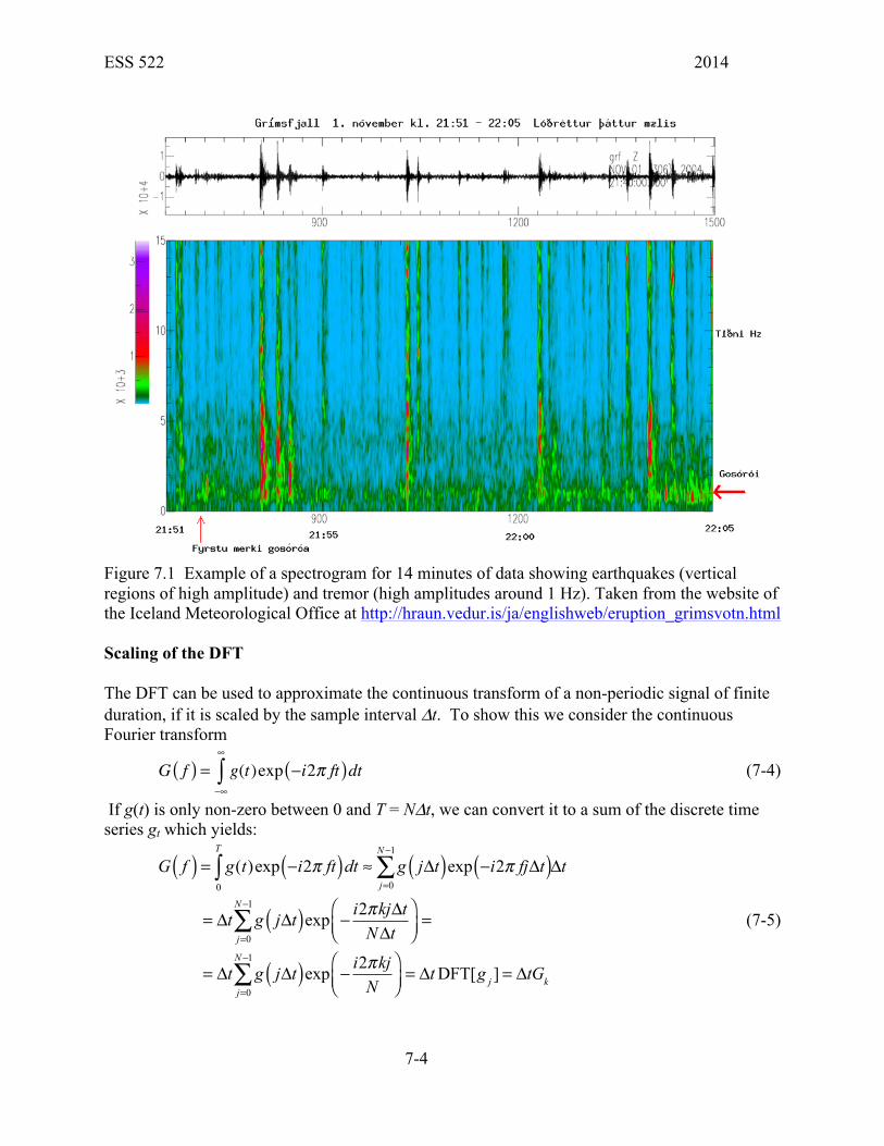
Figure 7.1 Example of a spectrogram for 14 minutes of data showing earthquakes (vertical regions of high amplitude) and tremor (high amplitudes around 1 Hz). Taken from the website of the Iceland Meteorological Office at http://hraun.vedur.is/ja/englishweb/eruption_grimsvotn.html Scaling of the DFT The DFT can be used to approximate the continuous transform of a non-periodic signal of finite duration, if it is scaled by the sample interval Δt. To show this we consider the continuous Fourier transform

G f( ) = g(t)exp −i2π ft( )dt−∞

∞

∫ (7-4)

If g(t) is only non-zero between 0 and T = NΔt, we can convert it to a sum of the discrete time series gt which yields:

G f( ) = g(t)exp −i2π ft( )dt0

T

∫ ≈ g jΔt( )exp −i2π fjΔt( )j=0

N−1

∑ Δt

= Δt g jΔt( )exp − i2πkjΔtNΔt

⎛⎝⎜

⎞⎠⎟j=0

N−1

∑ =

= Δt g jΔt( )exp − i2πkjN

⎛⎝⎜

⎞⎠⎟j=0

N−1

∑ = ΔtDFT[g j ] = ΔtGk

(7-5)

ESS 522 2014

7-5

where f = k/NΔt and we have assumed the version of the discrete Fourier transform used in Matlab with the 1/N scaling in the inverse transform. That is

Gk = gj exp −2πikjN

⎛⎝⎜

⎞⎠⎟j=0

N −1

∑ (7-6)

Scaling by the sample interval normalizes spectra to the continuous Fourier transform. Even if we are not interested in continuous Fourier transforms, this normalization allows us to directly compare spectral amplitudes obtained from discrete time series with different sample rates. Parseval’s Theorem Parsval’s theorem states that the energy of a signal, that is the integral (or sum) of the square of the signal, is equal to the integral (or sum) of the square of its Fourier transform Consider a signal of infinite duration. For the Fourier transform to be convergent the energy of the time series, E must be bounded

2( )E g t dt∞

−∞

= < ∞∫ (7-7)

The inverse Fourier transform for a continuous series is

g t( ) == G( f )exp i2π ft( )df−∞

∞

∫ (7-8)

If we substitute this for one g(t) term in equation (7-7) we get

2( ) ( ) ( ) exp( 2 )E g t dt g t G f i ft df dtπ∞ ∞ ∞

−∞ −∞ −∞

⎡ ⎤= = ⎢ ⎥

⎣ ⎦∫ ∫ ∫ (7-8)

By reversing the order of integration, we can write

( ) ( ) ( )22( ) ( ) ( ) exp( 2 ) *E g t dt G f g t i ft dt df G f G f df G f dfπ∞ ∞ ∞ ∞ ∞

−∞ −∞ −∞ −∞ −∞

⎡ ⎤= = = =⎢ ⎥

⎣ ⎦∫ ∫ ∫ ∫ ∫ (7-9)

where G* is the complex conjugate (Remember that for a complex variable we can write G = a + ib , G* = a − ib , andGG* = a2 + b2 ). We can think of g(t)2 as the distribution of ‘energy’ in the time domain and |G(f)|2 as the distribution of energy in the frequency domain. Now for a discrete time series which we assume represents a discrete version of a continuous time series that is zero outside the limits of the discrete time series, we can write the time domain representation of the energy as expressed in equation (7-7) as

1

2 2

00

( ) ( )T N

jE g t dt g j t t

−

=

= ≈ Δ Δ∑∫ (7-9)

The amplitude of time samples can be considered to be in units of energy / unit time interval . In the frequency domain we get a discrete version of equation (7-9)

( )1 1 22 2 2

Discrete,0 0( )

N N

kk k

E G f df G k f f t G f∞ − −

= =−∞

= = Δ Δ = Δ Δ∑ ∑∫ (7-10)

where the Δt2 in the right hand term adjusts the scaling of the discrete Fourier transform as required by equation (7-5).

ESS 522 2014

7-6

The units for the continuous Fourier transform, G(f) are energy /unit of frequency but for the

discrete Fourier transform they are energy /total spectral width of the DFT since the term 1/Δt is the total spectral width. Absolute Spectral Amplitudes In many applications we have no interest in the absolute values of the spectral amplitudes - We are either interested in relative values (which frequencies dominate a spectra) or we just want to manipulate a signal in the frequency domain (e.g, convolve or filter it) before returning to the time domain. However, if you are making use of the absolute spectral values you need to be careful to: 1. Scale the tapers used to minimize spectral leakage so that their root mean squared amplitude is unity. Otherwise the tapers will rescale the data. 2. Scale the discrete amplitude spectra with Δt (equation 7-3) and power spectra with Δt2 so that they have the same units as their continuous spectra. 3. Understand how the apparatus that recorded the digital data responds to different frequencies (i.e., know its impulse response) and apply the appropriate correction so that your spectra are in the units of physical interest.