6.3 Inverse Laplace Transforms - University of Albertacsproat/Homework/MATH 334/Chapter...Example...

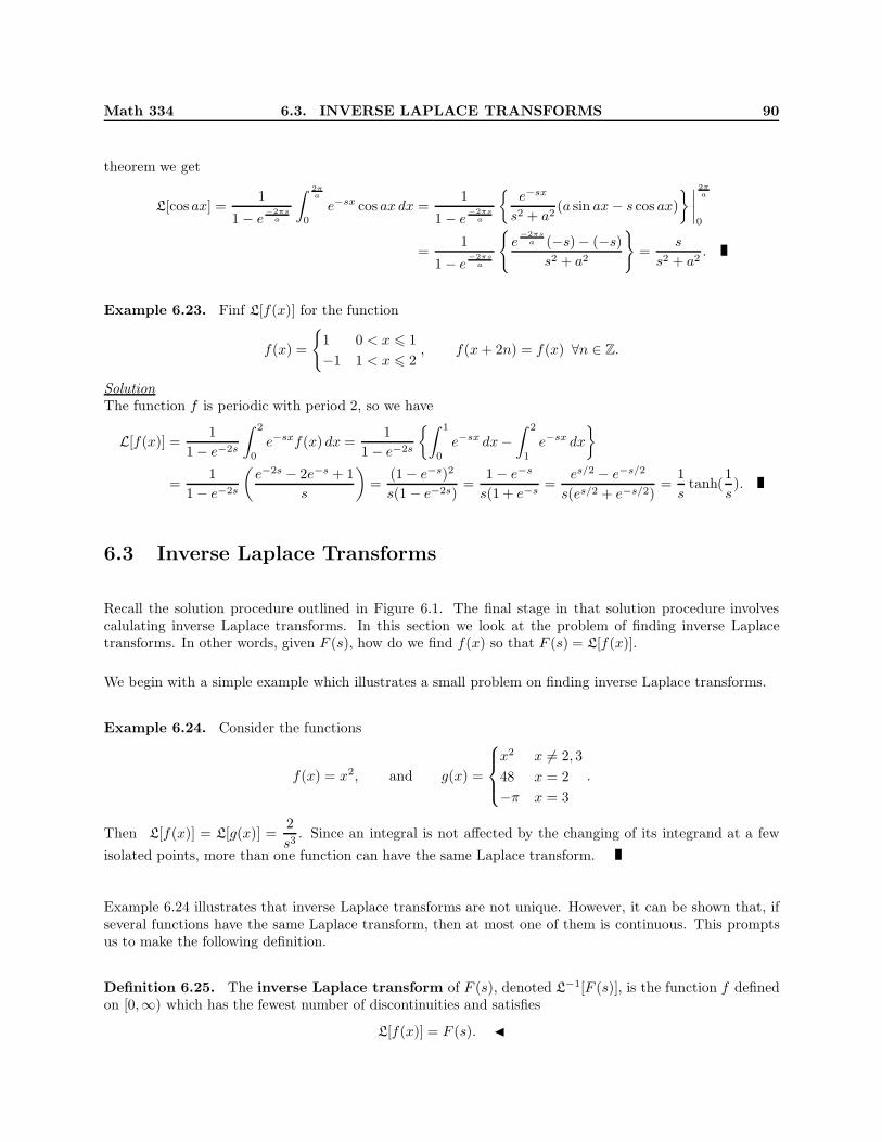
Math 334 6.3. INVERSE LAPLACE TRANSFORMS 90

theorem we get

L[cos ax] =1

1 − e−2πs

a

∫ 2π

a

0

e−sx cos ax dx =1

1 − e−2πs

a

{

e−sx

s2 + a2(a sin ax − s cos ax)

}∣

∣

∣

∣

2π

a

0

=1

1 − e−2πs

a

{

e−2πs

a (−s)− (−s)

s2 + a2

}

=s

s2 + a2.

Example 6.23. Finf L[f(x)] for the function

f(x) =

{

1 0 < x 6 1

−1 1 < x 6 2, f(x + 2n) = f(x) ∀n ∈ Z.

SolutionThe function f is periodic with period 2, so we have

L[f(x)] =1

1 − e−2s

∫ 2

0

e−sxf(x) dx =1

1 − e−2s

{∫ 1

0

e−sx dx −

∫ 2

1

e−sx dx

}

=1

1 − e−2s

(

e−2s − 2e−s + 1

s

)

=(1− e−s)2

s(1 − e−2s)=

1 − e−s

s(1 + e−s=

es/2 − e−s/2

s(es/2 + e−s/2)=

1

stanh(

1

s).

6.3 Inverse Laplace Transforms

Recall the solution procedure outlined in Figure 6.1. The final stage in that solution procedure involvescalulating inverse Laplace transforms. In this section we look at the problem of finding inverse Laplacetransforms. In other words, given F (s), how do we find f(x) so that F (s) = L[f(x)].

We begin with a simple example which illustrates a small problem on finding inverse Laplace transforms.

Example 6.24. Consider the functions

f(x) = x2, and g(x) =

x2 x 6= 2, 3

48 x = 2

−π x = 3

.

Then L[f(x)] = L[g(x)] =2

s3. Since an integral is not affected by the changing of its integrand at a few

isolated points, more than one function can have the same Laplace transform.

Example 6.24 illustrates that inverse Laplace transforms are not unique. However, it can be shown that, ifseveral functions have the same Laplace transform, then at most one of them is continuous. This promptsus to make the following definition.

Definition 6.25. The inverse Laplace transform of F (s), denoted L−1[F (s)], is the function f defined

on [0,∞) which has the fewest number of discontinuities and satisfies

L[f(x)] = F (s). ◭


Example 6.26.

1. L−1[

2

s3] = x2.

2. L−1[

s

s2 + 9] = cos 3x.

3. L−1[

s − 1

s2 − 2s + 5] = L

−1[s − 1

(s− 1)2 + 4] = ex

L−1[

s

s2 + 4] = ex cos 2x. (using property 1 of Theorem

6.17 in reverse)

The inverse Laplace transform is a linear operator.

Theorem 6.27.

If L−1[F (s)] and L

−1[G(s)] exist, then L−1[αF (s) + βG(s)] = αL

−1[F (s)] + βL−1[G(s)].

ProofStarting from the right hand side we have

L[αL−1[F (s)] + βL

−1[G(s)]] = αL[L−1[F (s)]] + βL[L−1[G(s)]] = αF (s) + βG(s).

The result follows.

Most of the properties of the Laplace transform can be reversed for the inverse Laplace transform.

Theorem 6.28.

If L−1[F (s)] = f(x), then the following hold:1. L

−1[F (s + a)] = e−axf(x);2. L

−1[sF (s)] = f ′(x), if f(0) = 0;

3. L−1[

1

sF (s)] =

∫ x

0

f(t) dt;

4. L−1[e−asF (s)] = ua(x) f(x− a).

Proof1. L[e−axf(x)] = F (s + a) from Theorem 6.17, property 1. The result follows.

2. L[f ′(x))] = −f(0) + sF (s) from Theorem 6.17, property 4. The result follows.

3. L[

∫ x

0

f(t) dt] =1

sF (s), from Theorem 6.17, property 5. The result follows.

4. L[ua(x)f(x− a)] = e−asL[f(x)] = e−asF (s), from Theorem 6.19. The result follows.

Example 6.29. Find L−1[

1

s(s2 + 1)].

Solution

We can write1

s(s2 + 1)=

1

sF (s), where F (s) =

1

s2 + 1. Then f(x) = L

−1[F (s)] = sinx, so we get

L−1[

1

s(s2 + 1)] = L

−1[1

sF (s)] =

∫ x

0

f(t) dt =

∫ x

0

sin t dt = 1 − cosx.



1

s(s2 + +2s + 5)].

Solution

L−1[

1

s(s2 + 2s + 5)] = L

−1[1

(s + 1)2 + 4] = e−x

L−1[

1

s2 + 4] =

1

2e−x sin 2x.


1 + e−s

s2].

Solution

L−1[

1 + e−s

s2] = L

−1[1

s2+

e−s

s2] = L

−1[1

s2] + L

−1[e−s

s2] = x + u1(x)(x− 1).


4e−2s

s2 + 16].

Solution

L−1[

4e−2s

s2 + 16] = L

−1[e−2s ·4

s2 + 16] = u2(x)L−1[

4

s2 + 16] = u2(x) sin 4x.

Many transforms that one encounters are of the form F (s) =P (s)

Q(s), where P and Q are polynomials in s

with deg{Q} > deg{P }. To evaluate L−1[F (s)], one writes

P (s)

Q(s)in terms of partial fractions.

Example 6.33 (distinct linear factors). Find L−1[

7s − 1

(s + 1)(s + 2)(s− 3)].

SolutionWe write the expression in the form

7s − 1

(s + 1)(s + 2)(s− 3)=

A

s + 1+

B

s + 2+

C

s − 3.

Solving for the constants yields: A = 2, B = −3, and C = 1. Thus, we get

L−1[

7s− 1

(s + 1)(s + 2)(s− 3)] = L

−1[2

s + 1] − L

−1[3

s + 2] + L

−1[1

s − 3] = 2e−x − 3e−2x + e3x.

Example 6.34 (repeated linear factors). Find L−1[

s2 + 9s + 2

(s − 1)2(s + 3)].


s2 + 9s + 2

(s − 1)2(s + 3)=

A

s − 1+

B

(s − 1)2+

C

s + 3.

Solving for the constants yields: A = 2, B = 3, and C = −3. Thus, we get

L−1[

s2 + 9s + 2

(s− 1)2(s + 3)] = L

−1[2

s − 1] + 3L

−1[1

(s − 1)2] − L

−1[1

s + 3] = 2e−x + 3xex − e−3x.

Math 334 6.4. APPLICATIONS TO DIFFERENTIAL EQUATIONS 93

Example 6.35 (quadratic factors). Find L−1[

2s2 + 10s

s2 − 2s + 5(s + 1)].


L−1[

2s2 + 10s

s2 − 2s + 5(s + 1)] =

A(s− 1) + B

(s − 1)2 + 4+

C

s + 1.

Solving for the constants yields: A = 3, B = 8, and C = −1. Thus, we get

L−1[

2s2 + 10s

s2 − 2s + 5(s + 1)] = 3L

−1[s − 1

(s − 1)2 + 4] + 4L

−1[2

(s − 1)2 + 4] − L

−1[1

s + 1]

= 3ex cos 2x + 4ex sin 2x− e−x.

6.4 Applications to Differential Equations

The easiest way to see how to apply Laplace transforms to differential equations is to work through someexamples.

Example 6.36. Solve the following initial value problem:

y′′ − y′ = 2x, y(0) = 1, y′(0) = −2.

SolutionMethod 1 (the old approach)First solve the homogeneous equation: y′′ − y = 0.

y = erx =⇒ r2 − r = 0 =⇒ r = 0, 1 =⇒ yh(x) = c1 + c2ex.

Now look for a particular solution: yp(x) = x(Ax + B) = Ax2 + Bx. Plug into the DE to get

y′′

p − y′

p = 0 =⇒

{

2A − B = 0

−2A = 2=⇒

{

A = −1

B = −2=⇒ yp(x) = −x2 − 2x.

Thus, we havey(x) = c1 + c2e

x − x2 − 2x, y′(x) = c2ex − 2x− 2.

Apply the initial conditions:

y(0) = 1y′(0) = −2

}

=⇒

{

c1 + c2 = 1

c2 − 2 = −2=⇒

{

c1 = 1

c2 = 0=⇒ y(x) = 1 − x2 − 2x .

Method 2 (using Laplace transforms)Take Laplace transforms of the DE:

L[y′′] − L[y′] = 2L[x] =⇒[

s2Y (s) − sy(0)− y′(0)]

− [sY (s) − y(0)] =2

s2

=⇒ s2Y (s) − s + 2 − sY (s) + 1 =2

s2

=⇒ Y (s) =s3 − 3s2 + 2

s3(s − 1)=

(s − 1)(s2 − 2s− 2)

s3(s − 1)=

1

s−

2

s2−

2

s3


Finally, taking the inverse Laplace transform, we arrive at the final solution:

y(x) = L−1[Y (s)] = 1 − 2x − x2.


y′′ − 2y′ + 5y = −8e−x, y(0) = 2, y′(0) = 12.

SolutionTake Laplace transforms of the DE:

L[y′′] − 2L[y′] + 5L[y] = −8L[e−x] =⇒[

s2Y (s)− sy(0)− y′(0)]

− 2 [sY (s)− y(0)] + 5Y (s) =2

s2

=⇒ s2Y (s)− 2s − 12− 2sY (s) + 4 + 5Y (s) =−8

s + 1

=⇒ Y (s) =2s2 + 10s

(s2 − 2s + 5)(s + 1)

=⇒ Y (s) = 3(s − 1)

(s− 1)2 + 4− 4

2

(s− 1)2 + 4−

1

s + 1.


y(x) = 3ex cos 2x + 4ex sin 2x− e−x.


y′′ − 2y′ + 5y = −8e7−x, y(7) = 2, y′(7) = 12.

SolutionIt appears that we can not use Laplace transforms since L[y′] = sY (s) − y(0), and we don’t know y(0).But we can get around this by moving the initial point (in this case x0 = 7) to the origin by means of atranslation.

Let t = x − 7 and w(t) = y(x). Then we get

w′(t) = y′(x), w′′(t) = y′′(x), w(0) = y(7), w′(0) = y′(7),

so, the initial value problem becomes

w′′ − 2w′ + 5w = −8e−t, w(0) = 2, w′(0) = 12.

This is just the initial value problem we had in Example 6.40. The solution is

w(t) = 3et cos 2t + 4et sin 2t − e−t.

The solution to the original problem is

y(x) = w(x − 7) = 3ex−7 cos[2(x− 7)] + 4ex−7 sin[2(x− 7)] − e−(x−7).

Next we consider an initial value problem with discontinuous forcing.



y′′ + 4y = g(x), y(0) = 0, y′(0) = 0, where g(x) =

1 0 < x < 1

−1 1 < x < 2

0 x > 2

.

SolutionWe can re-write g as follows: g(x) = 1[u0(x) − u1(x)] − 1[u1(x) − u2(x)] = u0(x) − 2u1(x) + u2(x). Thenwe have

G(s) = L[g(x)] = L[u0(x)]− 2L[u1(x)] + L[u2(x)] =1

s− 2

e−s

s+

e−2s

s.

Take Laplace transforms of the DE:

L[y′′] + 4L[y] = L[g(x)] =⇒[

s2Y (s) − sy(0)− y′(0)]

+ 4Y (s) = G(s)

=⇒ s2Y (s) + 4Y (s) = G(s)

=⇒ Y (s) =G(s)

s2 + 4=

1

s(s2 + 4)− 2

e−s

s(s2 + 4)+

e−2s

s(s2 + 4)

=⇒ Y (s) = F (s)− 2e−sF (s) + e−2sF (s),

where

F (s) =1

s(s2 + 4)=

1

4

(

1

s−

s

s2 + 4

)

.

Thus,

f(x) = L−1[F (s)] =

1

4(1− cos 2x).


y(x) = L−1[Y (s)] = L

−1[F (s)] − 2L−1[e−sF (s)] + L

−1[e−2sF (s)]

= f(x)− 2u1(x)f(x− 1) + u2(x)f(x− 2)

=1

4{1 − cos 2x− 2u1(x)(1− cos[2(x − 1)]) + u2(x)(1− cos[2(x − 2)])} .

Now we consider an ODE with variable coefficients.


y′′ + 2xy′ − 4y = 1, y(0) = 0, y′(0) = 0.

SolutionTake Laplace transforms of the DE:

L[y′′] + 2L[xy′] − 4L[y] = L[1] =⇒[

s2Y (s) − sy(0)− y′(0)]

− 2d

ds[sY (s) − y(0)]− 4Y (s) =

1

s

=⇒ s2Y (s) − 2[sY ′(s) + Y (s)] − 4Y (s) =1

s

=⇒ Y ′(s) +

(

3

s−

s

2

)

Y (s) =−1

2s2.

Math 334 6.5. CONVOLUTION 96

This is a linear ODE in Y (s). Look for an integrating factor µ:

µ′

µ=

3

s−

s

2=⇒ lnµ = 3 ln s −

s2

4=⇒ µ = s3e−s2/4.

The ODE for Y becomes:

d

ds[µY (s)] = µ

(

Y ′(s) +µ′

µY (s)

)

= −µ

2s2= −

s

2e−s2/4.

Integrating yields:

µY (s) = −

∫

s

2e−s2/4 ds = e−s2/4 + C =⇒ Y (s) =

1

s3+

C

s3es2/4.

It remains to determin the value of the constant if integration C. There is no auxiliary condition inheritedfrom the original ODE. To get an appropriate condition to enable us to determine C, we utilize Theorem6.12 that states that Y (s) → 0 as s → ∞. Therfore

lims→∞

Y (s) = 0 =⇒ C = 0 =⇒ Y (s) =1

s3.


y(x) = L−1[

1

s3] =

x2

2.

We can summarize the application of Laplace transforms to differential equations as follows.

1. For an ODE with constant coefficients, the equation for the Laplace transform is of the form AY = B.

2. For an ODE with polynomial coefficients in x, the equation for the Laplace transform is an ODE withpolynomial coefficients in s.

3. If the coefficient functions of the ODE are liear in x, the ODE for Y is a first order ODE.

4. The auxiliary condition to use when solving a first order ODE in Y is lims→∞

Y (s) = 0.

6.5 Convolution

Consider the following initial value problem:

y′′ + y = g(x), y(0) = y′(0) = 0.

Take the Laplace transform of the equation to get:

s2Y (s)− sy(0)− y′(0) + Y (s) = G(s) =⇒ Y (s) =G(s)

s2 + 1= F (s)G(s), where F (s) =

1

s2 + 1.

We would like to express the solution y(x) in terms of f(x) and g(x), i.e. we would like to express L−1[F (s)G(s)]

in terms of L−1[F (s)] and L

−1[G(s)]. To do this, we define a special type of product of functions. Letf, g ∈ PC(0,∞).

Math 334 6.5. CONVOLUTION 97

Definition 6.41. The convolution of f and g, denoted f ∗ g, is defined as:

(f ∗ g)(x) :=

∫ x

0

f(x − t)g(t) dt.

Example 6.42.

(1) 1 ∗ x =

∫ x

0

1 · t dt =x2

2.

(2) x ∗ x2 =

∫ x

0

(x− t) · t2 dt =x4

12.

Theorem 6.43.

The convolution product satisfies the following properties:1. f ∗ g = g ∗ f ; (convolution product is commutative)2. f ∗ (g + h) = f ∗ g + f ∗ h; (convolution product is distributive over addition)3. f ∗ (g ∗ h) = (f ∗ g) ∗ h; (convolution product is associative)4. f ∗ 0 = 0.

ProofExercise.

Remark. While the convolution product has many of the properties of ordinary multiplication of functions,it different in that it has no multiplicative identity element, i.e. there is no function g with the property thatg ∗ f 6= f for all funtions f . ◭

Theorem 6.44.

If (i) f, g ∈ PC(0,∞);(ii) F (s) = L[f(x)] and G(s) = L[g(x)], then

L[f ∗ g] = F (s)G(s), or equivalently L−1[F (s)G(s)] = (f ∗ g)(x).

Proof

L[f ∗ g] =

∫

∞

0

e−sx(f ∗ g)(x) dx =

∫

∞

0

e−sx

∫ x

0

f(x− t)g(t) dt dx

=

∫

∞

0

∫

∞

t

e−sxf(x − t)g(t) dx dt =

∫

∞

0

∫

∞

0

e−s(ξ+t)f(ξ)g(t) dξ dt

=

(∫

∞

0

e−sξf(ξ) dξ

)(∫

∞

0

e−stg(t) dt

)

= F (s)G(s).


1

s(s2 + 4)].

SolutionMethod 1 (the old approach)

L−1[

1

s(s2 + 4)] = L

−1[1

4

(

1

s−

s

s2 + 4

)

] =1

4(1 − cos 2x).

Method 2 (using convolution)

Math 334 6.6. THE DELTA FUNCTION 98

L−1[

1

s(s2 + 4)] =

1

2L−1[

1

s] ∗ L

−1[2

s2 + 4] =

1

2

∫ x

0

L−1[

1

s](x − t)L−1[

2

s2 + 4](t) dt

=1

2

∫ x

0

1 · sin 2t dt = −1

4cos 2t

∣

∣

∣

∣

x

0

=1

4(1− cos 2x).

Now, returning to the origin problem:

y′′ + y = g(x), y(0) = y′(0) = 0.

The solution satisfies:

y(x) = L−1[

G(s)

s2 + 1] = g ∗ sin x =

∫ x

0

g(t) sin(x − t) dt.

Example 6.46. Solve the following integro-differential equation:

y′(x) = 1 − e−2x

∫ x

0

y(t)e2t dt, y(0) = 1.

SolutionThe equation may be written as

y′ = 1 −

∫ x

0

j(t)e−2(x−t) dt = 1 − y ∗ e−2x.

Taking Laplace transforms we get

sY (s)− y(0) =1

s−

Y (s)

s + 2=⇒ Y (s) =

s + 2

s(s + 1)=

2

s−

1

s + 1=⇒ y(x) = 2 − e−x.

6.6 The Delta Function

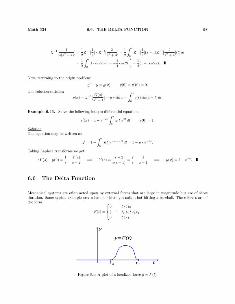
Mechanical systems are often acted upon by external forces that are large in magnitude but are of shortduration. Some typical example are: a hammer hitting a nail; a bat hitting a baseball. These forces are ofthe form

F (t) =

0 t < t0

(· · · ) t0 6 t 6 t1

0 t > t1

.

y

t

y=F(t)

t t 0 1

Figure 6.4: A plot of a localized force y = F (t).


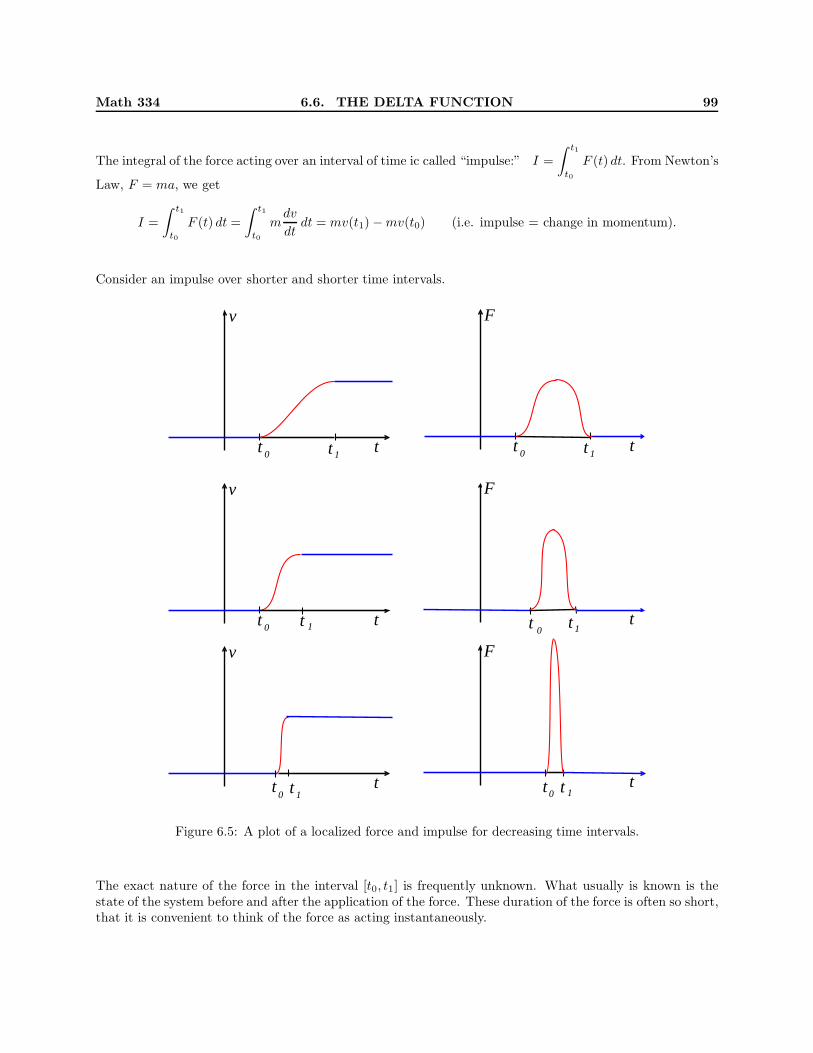
The integral of the force acting over an interval of time ic called “impulse:” I =

∫ t1

t0

F (t) dt. From Newton’s

Law, F = ma, we get

I =

∫ t1

t0

F (t) dt =

∫ t1

t0

mdv

dtdt = mv(t1) − mv(t0) (i.e. impulse = change in momentum).

Consider an impulse over shorter and shorter time intervals.

v

t t t 0 1 t t t 0 1

F

v

t t t 0 1 t t t 0 1

F

v

t t 0

t 1

F

t t 0 t 1

Figure 6.5: A plot of a localized force and impulse for decreasing time intervals.

The exact nature of the force in the interval [t0, t1] is frequently unknown. What usually is known is thestate of the system before and after the application of the force. These duration of the force is often so short,that it is convenient to think of the force as acting instantaneously.


v

t t t 0 1 t t t 0 1

F

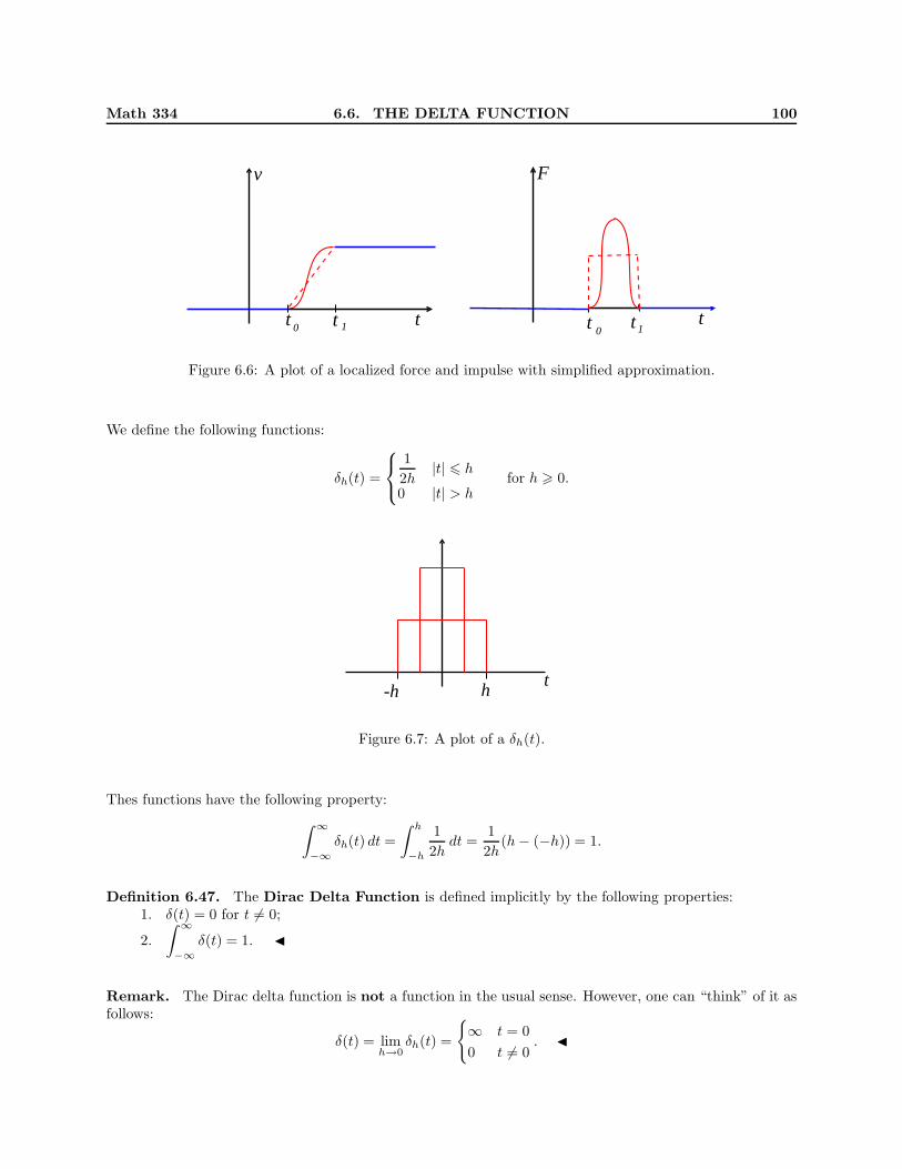
Figure 6.6: A plot of a localized force and impulse with simplified approximation.

We define the following functions:

δh(t) =

1

2h|t| 6 h

0 |t| > hfor h > 0.

t -h h

Figure 6.7: A plot of a δh(t).

Thes functions have the following property:

∫

∞

−∞

δh(t) dt =

∫ h

−h

1

2hdt =

1

2h(h − (−h)) = 1.

Definition 6.47. The Dirac Delta Function is defined implicitly by the following properties:1. δ(t) = 0 for t 6= 0;

2.

∫

∞

−∞

δ(t) = 1. ◭

Remark. The Dirac delta function is not a function in the usual sense. However, one can “think” of it asfollows:

δ(t) = limh→0

δh(t) =

{

∞ t = 0

0 t 6= 0. ◭


Theorem 6.48.

If f is continuous on (−∞,∞), then for any c ∈ R,

∫

∞

−∞

f(t) δ(t− c) dt = f(c).

ProofWe have

δh(t − c) =

1

2h|t − c| 6 h

0 |t − c| > h=

1

2hc − h 6 t 6 c + h

0 |t − c| > h.

Therefore

∫

∞

−∞

f(t)δ(t− c) dt = limh→0

∫

∞

−∞

f(t)δh(t − c) dt = limh→0

1

2h

∫ c+h

c−h

f(t) dt

= limh→0

1

2hf(c̄)(2h) for some c − h < c̄ < c + h (using the mean value theorem)

= limh→0

f(c̄) = f(c).

This is sometimes called the “sifting property” of the delta function since, from all possible values of f , it“sifts out” the value f(c).

Does the Dirac delta function have a Laplace transform? Yes it does, since

L[δ(t − c)] =

∫

∞

0

e−stδ(t − c) dt = e−sc.

Remark. Notice that for c = 0 we get L[δ(t)] = 1. This reinforces what was said earlier, namely that δ(t)is not a function in the usual sense, since, for a normal function we have

lims→∞

F (s) = 0, but for the delta function we have lims→∞

L[δ(t)] 6= 0. ◭


y′′ + y = 4δ(t− 2π), y(0) = y′(0) = 0.

SolutionTaking Laplace transforms we get,

s2Y (s)− sy(0) − y′(0) + Y (s) = 4e−2πs =⇒ Y (s) =4e−2πs

s2 + 1.

Taking inverse Laplace transforms we get

y(t) = u2π(t) sin(t − 2π) = u2π(t) sin t =

{

0 0 6 t < 2π

sin t t > 2π.

6.3 Inverse Laplace Transforms - University of Albertacsproat/Homework/MATH 334/Chapter...Example...

Documents

Transcript of 6.3 Inverse Laplace Transforms - University of Albertacsproat/Homework/MATH 334/Chapter...Example...