6.231 DYNAMIC PROGRAMMING

LECTURE 23

LECTURE OUTLINE

• Additional topics in ADP

• Stochastic shortest path problems

• Average cost problems

• Generalizations

• Basis function adaptation

• Gradient-based approximation in policy space

• An overview

1

REVIEW: PROJECTED BELLMAN EQUATION

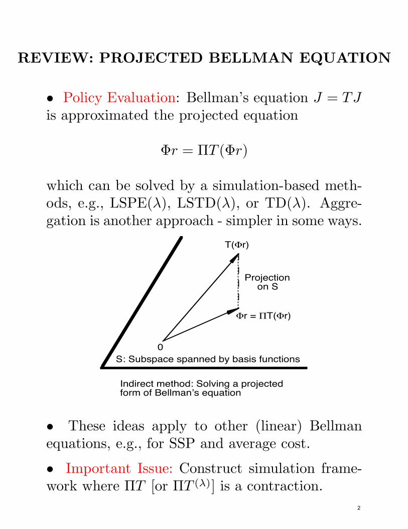
• Policy Evaluation: Bellman’s equation J = TJis approximated the projected equation

Φr = ΠT (Φr)

which can be solved by a simulation-based meth-ods, e.g., LSPE(λ), LSTD(λ), or TD(λ). Aggre-gation is another approach - simpler in some ways.

S: Subspace spanned by basis functions

T(Φr)

0

Φr = ΠT(Φr)

Projectionon S

Indirect method: Solving a projected form of Bellmanʼs equation

• These ideas apply to other (linear) Bellmanequations, e.g., for SSP and average cost.

• Important Issue: Construct simulation frame-work where ΠT [or ΠT (λ)] is a contraction.

2

STOCHASTIC SHORTEST PATHS

• Introduce approximation subspace

S = {Φr | r ∈ ℜs}

and for a given proper policy, Bellman’s equationand its projected version

J = TJ = g + PJ, Φr = ΠT (Φr)

Also its λ-version∞

Φr = ΠT (λ)(Φr), T (λ) = (1− λ)∑

λtT t+1

t=0

• Question: What should be the norm of projec-tion? How to implement it by simulation?

• Speculation based on discounted case: It shouldbe a weighted Euclidean norm with weight vectorξ = (ξ1, . . . , ξn), where ξi should be some type oflong-term occupancy probability of state i (whichcan be generated by simulation).

• But what does “long-term occupancy probabil-ity of a state” mean in the SSP context?

• How do we generate infinite length trajectoriesgiven that termination occurs with prob. 1?

3

SIMULATION FOR SSP

• We envision simulation of trajectories up totermination, followed by restart at state i withsome fixed probabilities q0(i) > 0.

• Then the “long-term occupancy probability ofa state” of i is proportional to

∞

q(i) =∑

qt(i), i = 1, . . . , n,t=0

where

qt(i) = P (it = i), i = 1, . . . , n, t = 0, 1, . . .

• We use the projection norm

‖J‖q =

√

√

√

√

n∑

q(i)i=1

(

J(i))2

[Note that 0 < q(i) < ∞, but q is not a prob.distribution.]

• We can show that ΠT (λ) is a contraction withrespect to ‖ · ‖q (see the next slide).

• LSTD(λ), LSPE(λ), and TD(λ) are possible.4

CONTRACTION PROPERTY FOR SSP

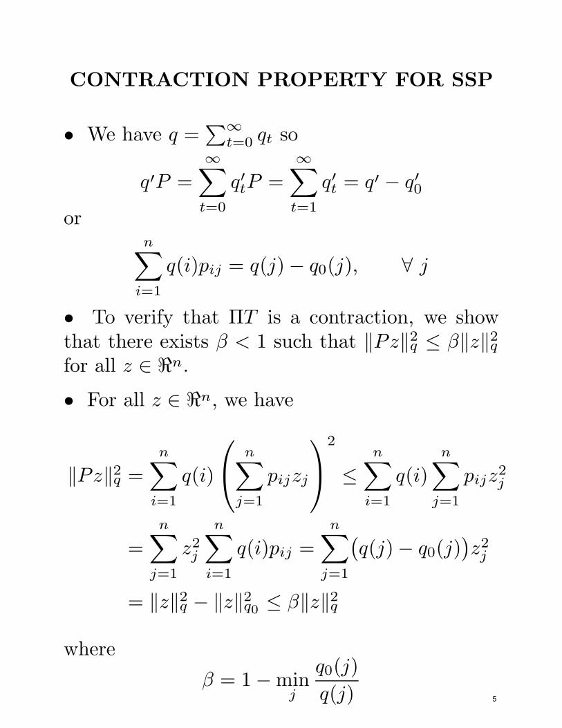
• We have q =∑∞

=0 qtt so∞ ∞

q′P =∑

q′tP =t=0

∑

q′ ′t = q′ q0

t=1

−or

n∑

q(i)pij = q(j) qi=1

− 0(j), ∀ j

• To verify that ΠT is a contraction, we showthat there exists β < 1 such that ‖Pz 2

q

n

‖ ≤ β‖z‖2qfor all z ∈ ℜ .

• For all z ∈ ℜn, we have

2n n n n

‖Pz‖2 =∑

q(i)

∑

p z

≤∑

q(i)∑

p z2q ij j ij j

i=1 j=1 i=1 j=1

n n n

=∑

z2j∑

q(i)pij =∑

(

q(j) jj=1 i=1 j 1

− q0( )=

)

z2j

= ‖z‖2q − ‖z‖2q0 ≤ β‖z‖2q

whereq )

β = 1− 0(jminj q(j) 5

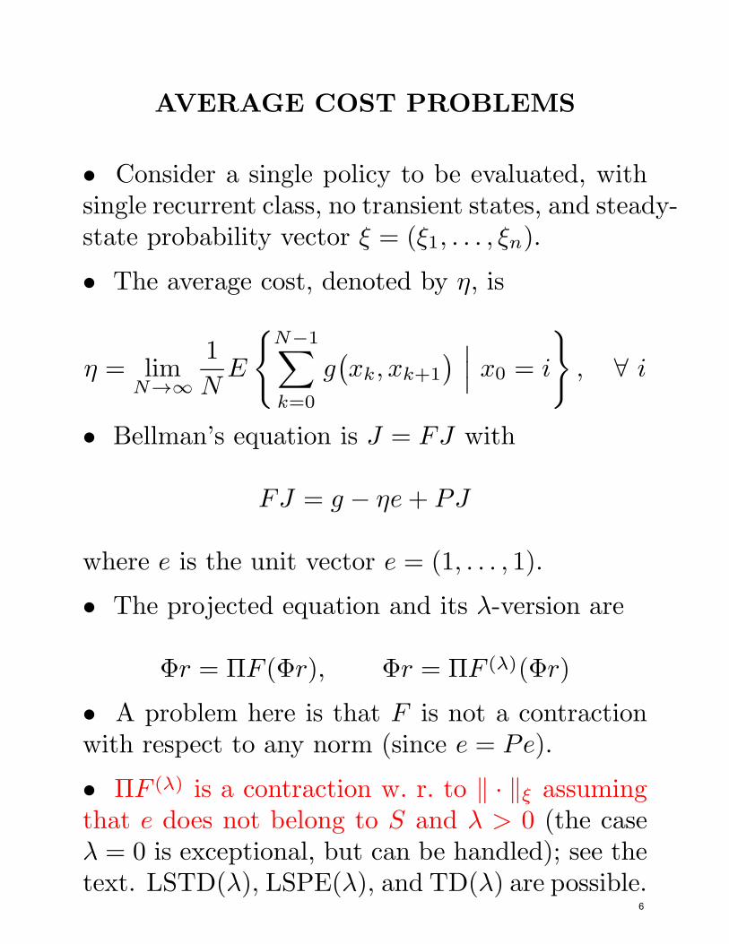
AVERAGE COST PROBLEMS

• Consider a single policy to be evaluated, withsingle recurrent class, no transient states, and steady-state probability vector ξ = (ξ1, . . . , ξn).

• The average cost, denoted by η, is

1η = lim

N→∞x

N

{

N−1

E g k, xk+1

k=0

}

∑

ati n

(

is J = FJ

)

• Bellman’s equ

∣

∣

∣

x0 = i , ∀ i

o with

FJ = g − ηe+ PJ

where e is the unit vector e = (1, . . . , 1).

• The projected equation and its λ-version are

Φr = ΠF (Φr), Φr = ΠF (λ)(Φr)

• A problem here is that F is not a contractionwith respect to any norm (since e = Pe).

• ΠF (λ) is a contraction w. r. to ‖ · ‖ξ assumingthat e does not belong to S and λ > 0 (the caseλ = 0 is exceptional, but can be handled); see thetext. LSTD(λ), LSPE(λ), and TD(λ) are possible.

6

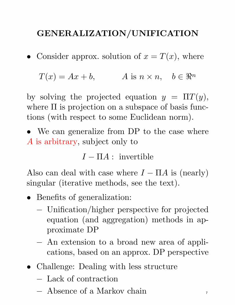
GENERALIZATION/UNIFICATION

• Consider approx. solution of x = T (x), where

T (x) = Ax+ b, A is n× n, b ∈ ℜn

by solving the projected equation y = ΠT (y),where Π is projection on a subspace of basis func-tions (with respect to some Euclidean norm).

• We can generalize from DP to the case whereA is arbitrary, subject only to

I −ΠA : invertible

Also can deal with case where I − ΠA is (nearly)singular (iterative methods, see the text).

• Benefits of generalization:

− Unification/higher perspective for projectedequation (and aggregation) methods in ap-proximate DP

− An extension to a broad new area of appli-cations, based on an approx. DP perspective

• Challenge: Dealing with less structure

− Lack of contraction

− Absence of a Markov chain 7

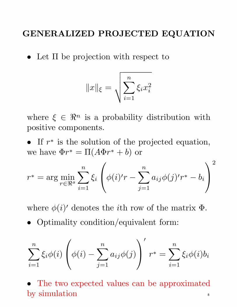
GENERALIZED PROJECTED EQUATION

• Let Π be projection with respect to

‖x‖ξ =

√

√

√

√

n∑

ξix2i

i=1

where ξ ∈ ℜn is a probability distribution withpositive components.

• If r∗ is the solution of the projected equation,we have Φr∗ = Π(AΦr∗ + b) or

2n n

r∗ = arg min ξ

∑

φ(i)′r −∑

a φ(j)′ ∗i ij r bi

r∈ℜs

i=1 j=1

−

where φ(i)′ denotes the ith row of the matrix Φ.

• Optimality condition/equivalent form:

′n n n∑

ξiφ(i)

φ(i)−∑

aijφ(j)

r∗ =∑

ξiφ(i)bii=1 j=1 i=1

• The two expected values can be approximatedby simulation 8

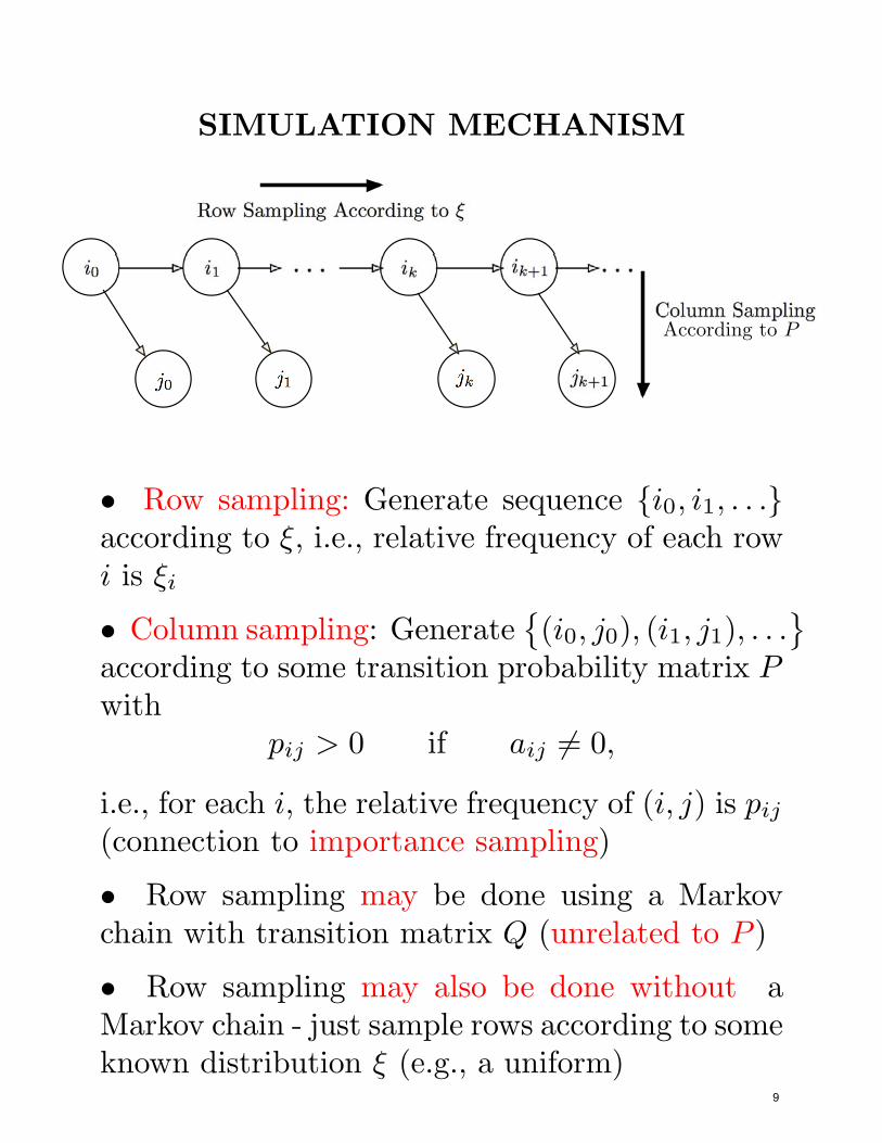
SIMULATION MECHANISM

i0 i1

j0 j1

ik ik+1

jk jk+1

. . . . . .

Column SamplingAccording to P

Row Sampling According to ξ (MaColumn Sampling According to

Roi0Row

i1w Sam

0

amp

j1plin

ikling Accordi

+1

Accordijk

According

+1

ng to+1

ng to Ac= ( ) Φ Πg Mar

• Row sampling: Generate sequence {i0, i1, . . .}according to ξ, i.e., relative frequency of each rowi is ξi

• Column sampling: Generate (i0, j0), (i1, j1), . . .according to some transition pr

{

obability matrix Pwith

}

pij > 0 if aij 6= 0,

i.e., for each i, the relative frequency of (i, j) is pij(connection to importance sampling)

• Row sampling may be done using a Markovchain with transition matrix Q (unrelated to P )

• Row sampling may also be done without aMarkov chain - just sample rows according to someknown distribution ξ (e.g., a uniform)

9

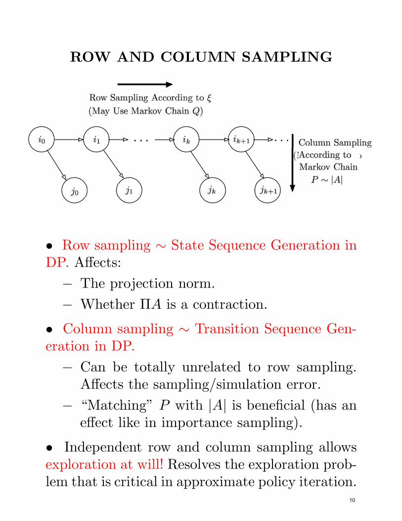
ROW AND COLUMN SAMPLING

Column Sampling

According to(May Use MarkoMarkov Chainov Chain

P ∼ |A|

i0 i1

j0 j1

ik ik+1

jk jk+1

. . . . . .

Row Sampling According to ξ (MaColumn Sampling According toξ (May Use Markov Chain Q)

to Markov Chain P ∼ |A|

Ac= ( ) Φ Πg Mar(Φ ) Subspaceto

Subspace Projectionk

ainjection on

Roi0Row

i1w Sam

0

amp

j1plin

ikling Accordi

+1

Accordijk

According

+1

ng to+1

ng to

• Row sampling ∼ State Sequence Generation inDP. Affects:

− The projection norm.

− Whether ΠA is a contraction.

• Column sampling ∼ Transition Sequence Gen-eration in DP.

− Can be totally unrelated to row sampling.Affects the sampling/simulation error.

− “Matching” P with |A| is beneficial (has aneffect like in importance sampling).

• Independent row and column sampling allowsexploration at will! Resolves the exploration prob-lem that is critical in approximate policy iteration.

10

LSTD-LIKE METHOD

• Optimality condition/equivalent form of pro-jected equation

′n n n∑

ξ ∗iφ(i)

φ(i)−∑

aijφ(j)

r =∑

ξiφ(i)bii=1 j=1 i=1

• The two expected values are approximated byrow and column sampling (batch 0 → t).

• We solve the linear equation

t

k

∑

φ(ik)=0

(

aφ(i )− ikjk

k φ(jk)pikjk

)′ t

rt =∑

φ(ik)bikk=0

• We have rt → r∗, regardless of ΠA being a con-traction (by law of large numbers; see next slide).

• Issues of singularity or near-singularity of I−ΠAmay be important; see the text.

• An LSPE-like method is also possible, but re-quires that ΠA is a contraction.

• nUnder the assumption j=1 |aij | ≤ 1 for all i,

there are conditions that g

∑

uarantee contraction ofΠA; see the text.

11

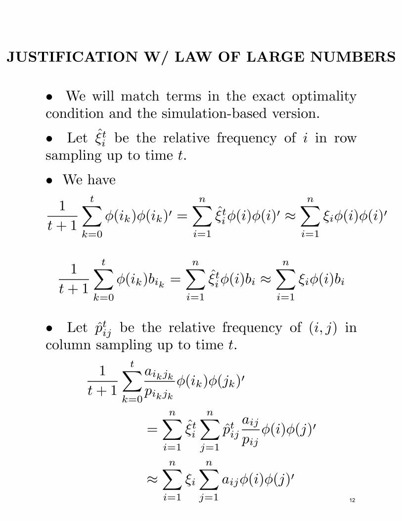
JUSTIFICATION W/ LAW OF LARGE NUMBERS

• We will match terms in the exact optimalitycondition and the simulation-based version.

• ˆLet ξti be the relative frequency of i in rowsampling up to time t.

• We have

1t n n

(+ 1

∑

ˆφ(ik)φ i ξtk)′ =t

∑

′ ′iφ(i)φ(i)

k=0 =1

≈∑

ξiφ(i)φ(i)i i=1

1t n n∑

ˆφ(i )b tk ik =

∑

ξiφ(i)bit+ 1k=0 i=1

≈∑

ξiφ(i)bii=1

• Let p̂tij be the relative frequency of (i, j) incolumn sampling up to time t.

1t

t+ 1k

∑aikjk

=0

φ(ik)φ(jk)′pikjk

n n∑

ˆ∑ aij

= ξti p̂tiji=1 j=1

φ(i)φ(j)′pij

n n

≈∑

ξ ′i

i=1

∑

aijφ(i)φ(j)j=1 12

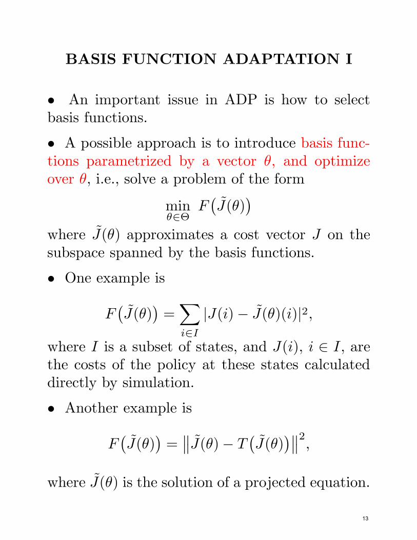
BASIS FUNCTION ADAPTATION I

• An important issue in ADP is how to selectbasis functions.

• A possible approach is to introduce basis func-tions parametrized by a vector θ, and optimizeover θ, i.e., solve a problem of the form

˜min F J(θ)θ∈Θ

˜where J(θ) approximates

(

a co

)

st vector J on thesubspace spanned by the basis functions.

• One example is

˜ ˜F J(θ) =i∈I

|J(i)− J(θ)(i)|2,

where I is

(

a sub

)

set o

∑

f states, and J(i), i ∈ I, arethe costs of the policy at these states calculateddirectly by simulation.

• Another example is

F(

˜ 2J(θ

)

=∥

∥ ˜ ˜) J(θ)− T J(θ) ,

˜where J(θ) is the solution of a p

(

rojec

)

t

∥

∥

ed equation.

13

BASIS FUNCTION ADAPTATION II

• Some optimization algorithm may be used to˜minimize F(

J(θ))

over θ.

• A challenge here is that the algorithm shoulduse low-dimensional calculations.

• One possibility is to use a form of random search(the cross-entropy method); see the paper by Men-ache, Mannor, and Shimkin (Annals of Oper. Res.,Vol. 134, 2005)

• Another possibility is to use a gradient method.For this it is necessary to estimate the partial

˜derivatives of J(θ) with respect to the componentsof θ.

• It turns out that by differentiating the pro-jected equation, these partial derivatives can becalculated using low-dimensional operations. Seethe references in the text.

14

APPROXIMATION IN POLICY SPACE I

• Consider an average cost problem, where theproblem data are parametrized by a vector r, i.e.,a cost vector g(r), transition probability matrixP (r). Let η(r) be the (scalar) average cost perstage, satisfying Bellman’s equation

η(r)e+ h(r) = g(r) + P (r)h(r)

where h(r) is the differential cost vector.• Consider minimizing η(r) over r. Other thanrandom search, we can try to solve the problemby a policy gradient method:

rk+1 = rk − γk∇η(rk)

• Approximate calculation of ∇η(rk): If ∆η, ∆g,∆P are the changes in η, g, P due to a small change∆r from a given r, we have

∆η = ξ′(∆g +∆Ph),

where ξ is the steady-state probability distribu-tion/vector corresponding to P (r), and all the quan-tities above are evaluated at r.

15

APPROXIMATION IN POLICY SPACE II

• Proof of the gradient formula: We have, by “dif-ferentiating” Bellman’s equation,

∆η(r)·e+∆h(r) = ∆g(r)+∆P (r)h(r)+P (r)∆h(r)

By left-multiplying with ξ′,

′∆ ( )· + ′∆ ( ) = ′ξ η r e ξ h r ξ ∆ ( )+∆ ( ) ( ) + ′g r P r h r ξ P (r)∆h(r)

Since ξ′∆η(r)

( )

· e = ∆η(r) and ξ′ = ξ′P (r), thisequation simplifies to

∆η = ξ′(∆g +∆Ph)

• Since we don’t know ξ, we cannot implement agradient-like method for minimizing η(r). An al-ternative is to use “sampled gradients”, i.e., gener-ate a simulation trajectory (i0, i1, . . .), and changer once in a while, in the direction of a simulation-based estimate of ξ′(∆g +∆Ph).

• Important Fact: ∆η can be viewed as an ex-pected value!

• Much research on this subject, see the text.

16

6.231 DYNAMIC PROGRAMMING

OVERVIEW-EPILOGUE

• Finite horizon problems

− Deterministic vs Stochastic

− Perfect vs Imperfect State Info

• Infinite horizon problems

− Stochastic shortest path problems

− Discounted problems

− Average cost problems

17

FINITE HORIZON PROBLEMS - ANALYSIS

• Perfect state info

− A general formulation - Basic problem, DPalgorithm

− A few nice problems admit analytical solu-tion

• Imperfect state info

− Reduction to perfect state info - Sufficientstatistics

− Very few nice problems admit analytical so-lution

− Finite-state problems admit reformulation asperfect state info problems whose states areprob. distributions (the belief vectors)

18

FINITE HORIZON PROBS - EXACT COMP. SOL.

• Deterministic finite-state problems

− Equivalent to shortest path

− A wealth of fast algorithms

− Hard combinatorial problems are a specialcase (but # of states grows exponentially)

• Stochastic perfect state info problems

− The DP algorithm is the only choice

− Curse of dimensionality is big bottleneck

• Imperfect state info problems

− Forget it!

− Only small examples admit an exact compu-tational solution

19

FINITE HORIZON PROBS - APPROX. SOL.

• Many techniques (and combinations thereof) tochoose from

• Simplification approaches

− Certainty equivalence

− Problem simplification

− Rolling horizon

− Aggregation - Coarse grid discretization

• Limited lookahead combined with:

− Rollout

− MPC (an important special case)

− Feature-based cost function approximation

• Approximation in policy space

− Gradient methods

− Random search

20

INFINITE HORIZON PROBLEMS - ANALYSIS

• A more extensive theory

• Bellman’s equation

• Optimality conditions

• Contraction mappings

• A few nice problems admit analytical solution

• Idiosynchracies of problems with no underlyingcontraction

• Idiosynchracies of average cost problems

• Elegant analysis

21

INF. HORIZON PROBS - EXACT COMP. SOL.

• Value iteration

− Variations (Gauss-Seidel, asynchronous, etc)

• Policy iteration

− Variations (asynchronous, based on value it-eration, optimistic, etc)

• Linear programming

• Elegant algorithmic analysis

• Curse of dimensionality is major bottleneck

22

INFINITE HORIZON PROBS - ADP

• Approximation in value space (over a subspaceof basis functions)

• Approximate policy evaluation

− Direct methods (fitted VI)

− Indirect methods (projected equation meth-ods, complex implementation issues)

− Aggregation methods (simpler implementa-tion/many basis functions tradeoff)

• Q-Learning (model-free, simulation-based)

− Exact Q-factor computation

− Approximate Q-factor computation (fitted VI)

− Aggregation-based Q-learning

− Projected equation methods for opt. stop-ping

• Approximate LP

• Rollout

• Approximation in policy space

− Gradient methods

− Random search

23

MIT OpenCourseWarehttp://ocw.mit.edu

6.231 Dynamic Programming and Stochastic ControlFall 2015

For information about citing these materials or our Terms of Use, visit: http://ocw.mit.edu/terms.