AQUACULTURE AND FISHERIES ECONOMICS

Acknowledgements

This course was authored by:

Dr. George Matiya

Aquaculture Department

Bunda College of Agriculture

Email: georgematiya@yahoo.co.uk

The course was reviewed by:

Dr Julius Mangisoni

University of Malawi, Bunda College

Email: hmangisoni@gmail.com

The following organisations have played an important role in facilitating the creation of this course:

1. The Association of African Universities through funding from DFID (http://aau.org/)

2. The Regional Universities Forum for Capacities in Agriculture, Kampala, Uganda (http://ruforum.org/)

3. Bunda College of Agriculture, University of Malawi, Malawi (http://www.bunda.luanar.mw/)

These materials have been released under an open license: Creative Commons Attribution 3.0 Unported License (https://creativecommons.org/licenses/by/3.0/). This means that we encourage you to copy, share and where necessary adapt the materials to suite local contexts. However, we do reserve the right that all copies and derivatives should acknowledge the original author.

1.0 Course Description

Aquaculture and Fisheries Economics course imparts knowledge and skills to enable learners

run their enterprises based on sound economic principles. For fisheries and aquaculture to

contribute significantly to food security and poverty alleviation, there is need for should be

pursued as business entities and hence the need to have a clear understanding of the

production and marketing concepts. Effective and efficient production and marketing systems

will help the different stakeholders understand the problems in fisheries and aquaculture which

would lead to sound decision making.

2.0 COURSE AIMSTo enable students develop a critical understanding of economic theories and their

applications in Aquaculture and Fisheries.

COURSE OBJECTIVES:By the end of the course students should be able to:

a) evaluate results from aquaculture and Fisheries analyses for policy decision making

b) analyze the essential elements of Aquaculture and Fisheries economics.c) assess different measures for evaluating Fisheries resource depletion for

management.d) synthesize potential risks involved in resource extractione) evaluate projects on Aquaculture and Fisheriesf) apply quality benefit and capital theories to quality relationships

2.0 Learning Outcomes

On successful completion of this the students will be able to:

Knowledge and understanding

analyze the essential elements of Aquaculture and Fisheries economics.

evaluate results from aquaculture and Fisheries analyses for policy decision making

Skills

apply quality benefit and capital theories to quality relationships

assess different measures for efficient fisheries and aquaculture production

management

synthesize potential risks involved in resource extraction

Attitude

Influence economic efficiency in fisheries and aquaculture production

TOPICS OF STUDY

1. REVIEW OF THE PRODUCTION FUNCTIONa. Definition of a Production Function

b. Physical and financial Quantities in a Production Function

c. Stages of the Production Function

d. Biological efficiency and economic efficiency

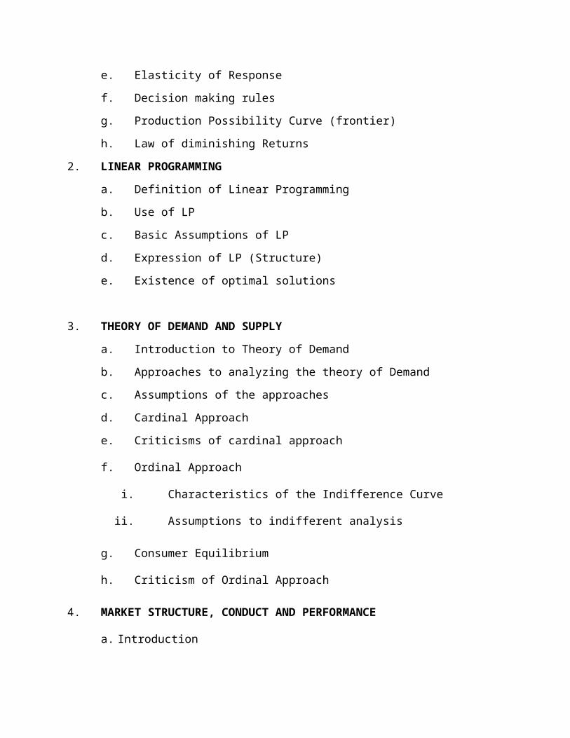
e. Elasticity of Response

f. Decision making rules

g. Production Possibility Curve (frontier)

h. Law of diminishing Returns

2. LINEAR PROGRAMMING

a. Definition of Linear Programming

b. Use of LP

c. Basic Assumptions of LP

d. Expression of LP (Structure)

e. Existence of optimal solutions

3. THEORY OF DEMAND AND SUPPLY

a. Introduction to Theory of Demand

b. Approaches to analyzing the theory of Demand

c. Assumptions of the approaches

d. Cardinal Approach

e. Criticisms of cardinal approach

f. Ordinal Approach

i. Characteristics of the Indifference Curve

ii. Assumptions to indifferent analysis

g. Consumer Equilibrium

h. Criticism of Ordinal Approach

4. MARKET STRUCTURE, CONDUCT AND PERFORMANCE

a. Introduction

b. Elements of Market Structure

i. Seller concentration,

ii. Product differentiation,

iii. Barriers to entry,

iv. Barriers to exit,

v. Buyer concentration,

vi. Growth rate of market demand.

c. Types of Market system

i. Perfect/ Pure Competitive Market system

ii. Assumptions for Pure Competitive Market system

iii. Supply Decisions under perfect competition

d. Imperfect Competition

I. Monopoly

i. Characteristics of a monopolist market

ii. Sources of monopoly power

iii. Criticisms of monopoly

iv. Interventions in a Monopoly market

II. Oligopoly Market

e. Market Conduct

f. Market Performance

5. TIME VALUE OF MONEY

a. Introduction to Time Value of Money

b. Future Value of Money

i. Future Value of a present sum

ii. Applicability

iii. Future Value of a Stream of Investments

iv. Equal payment-future value interest factors

v. Relationship between FIFr,n and EFIFr,n

c. Present value

i. Discounting

ii. Present value of a future sum

iii. Present value of a stream of Income

iv. Equal Periodic Income Flows

v. Relationship between FIF and PIF

6. COST BENEFIT THEORY

a. Introduction to Cost benefit theoryb. Steps in calculating Benefit-cost ratioc. Net Present Valued. Decision making rule

7. EFFICIENT MARKET HYPOTHESIS - EMHa. Definition of EMHb. The Effect of Efficiency: Non-Predictabilityc. Anomalies: The Challenge to Efficiencyd. The EMH Responsee. How Does a Market Become Efficient?f. Degrees of Efficiencyg. Random Walk Theory h. Conclusion

8. WELFARE ECONOMICSa. Introduction to Welfare economicsb. Approaches to studying welfare economicsc. Efficiency

d. Income distribution

PRACTICAL TOPICS

Problem sets and case studies related to topics covered in lectures.

INSTRUCTIONAL METHODOLOGY AND ASSESSMENT

As part of coursework lectures, tutorials, assignments as well field visits shall be conducted.

Assessment of the course will be in two parts namely a three-hour end of semester

examination (constituting 60% of the total marks) and Continuous assessment tests

(constituting 60% of the total marks) which shall include mid-semester examination and

assignments. The passing mark for the course shall be 60%.

RECOMMENDED TEACHING RESOURCES

Conrad, J.M. and Clark. C.W. (1999). Natural Resource Economics: Notes and Problems.

Cambridge University Press. Cambridge.

Jolly, C.M., and Clonts, H. A. (1993). Economics of Aquaculture. Food Products Press, an

Imprint of the Hearth Press, Inc.,

Perman, R., Y. Ma, J. M. and Common. M. (1999). Natural Resource and Environmental

Economics. Longman, Harlow.

Barry, P. J. (Ed.). (1984) Risk Management in Agriculture. Iowa State Press, Ames.

Conrad, J.M. (1999). Resource Economics. Cambridge University Press, Cambridge

Cornes, R.. and Sandler T. (1995). The Theory of Externalities, Public Goods, and Club

Goods. Cambridge University Press, Cambridge.

Dasgupta P. (2001). Human Well-being and the Natural Environment, Oxford

University Press, Oxford.

Debertin, D.L. (1986). Agricultural Production Economics. 3rd Edition. Privately published

(similar to the 1st edition of Debertin published by Macmillan).

Farris, P.L. 1983). Agricultural marketing research in perspective. The Iowa State

University Press, Ames.

Hansen, S. (1989). Debt for Nature Swaps: Overview and Discussion of Key Issues,

Ecological Economics 1:77-95.

Nordhaus W.D. (1993). Reflections on the Economics of Climate Change. Journal of

Economic Perspectives. Volume 2, Number 4, pp. 11-25.

Stern D, M. Common and Barbier. E (1996). Economic Growth and Environmental

Degradation: The Environmental Kuznets Curve and Sustainable Development, World

Development 247: 1151-1160

TOPIC 1: REVIEW OF PRODUCTION FUNCTION

In this topic, you will learn about the three stages of production function and how biological

efficiency differs from economic efficiency. it presented.

Learning Outcomes

Upon completion of this lesson you will be able to;

1 Describe the input –output relationship in aquaculture and fisheries production

functions.

2 Differentiate biological efficiency and economic efficiency.

3 Apply knowledge of production function in production of fish.

Key Terms: Elasticity, Efficiency, Production Possibility frontier, Law of Diminishing Returns

1.0 Introduction to Production Function

Production is the transformation of inputs into outputs. Inputs are the factors of production --

land, labor, and capital -- plus raw materials and business services while outputs are the

products. The relationship between the quantities of inputs and the maximum quantities of

outputs produced is called the "production function." How do these outputs change when the

input quantities vary? In the production we vary one variable input while holding the other

factors of production constant. For example vary the amount of feed while assuming the size of

the pond and labour as constant. This is done to analyze the effect of varying the feed on yield.

The production function relates the output of a firm to the amount of inputs being used. It

describes the rate at which resources are transformed into products

1.1 Presentation of Production Functions

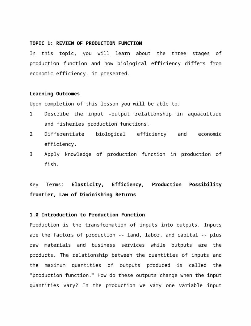
1.1.1 Tabular (Table 1)

Table showing production function in tabular form

Feed Yield(kg/ha) (kg)20 3740 13960 28880 469100 667120 864

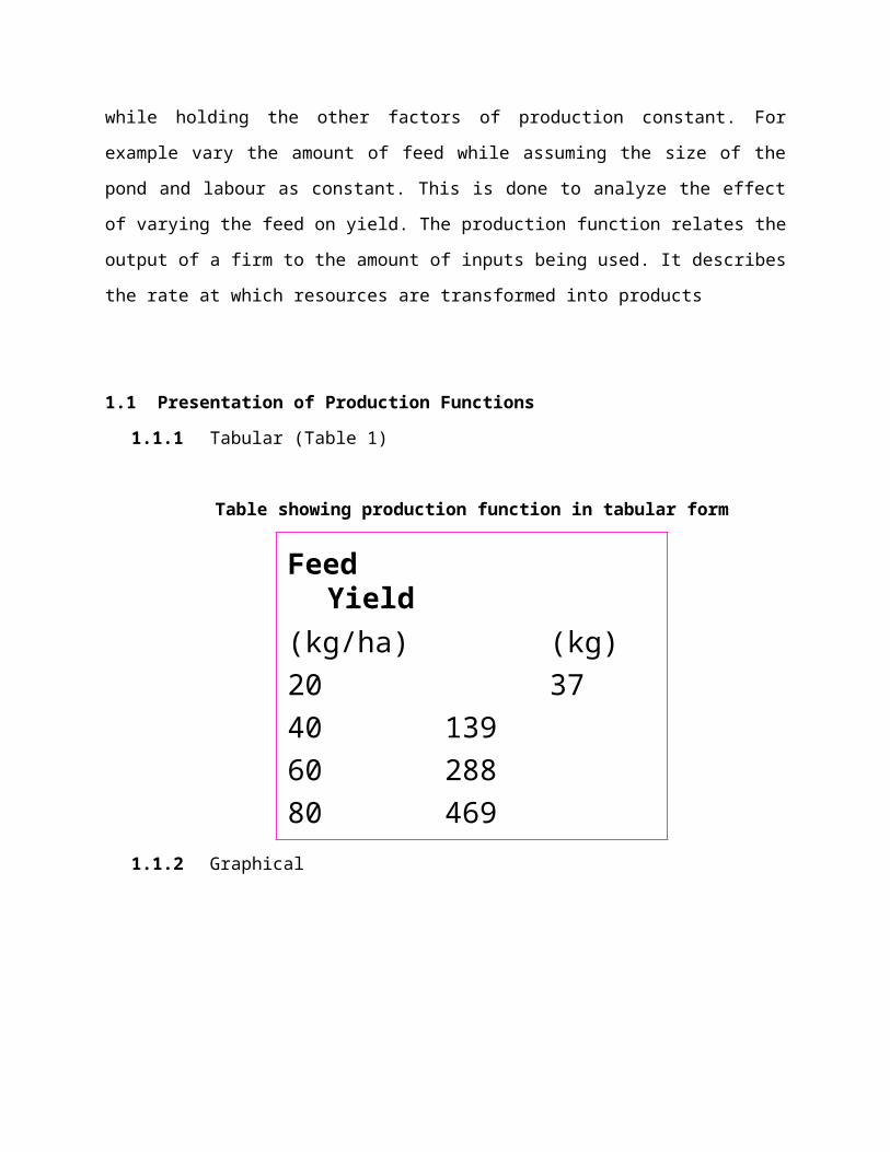
1.1.2 Graphical

source:

Fig: Graphs for TPP, APP and MPP

1.2 Physical and financial Quantities in a Production Function

1.2.1 TPP and TVP

Total Physical product (TPP) = total output or yield (Y) that can be attained by using the

variable input X1 and a set of fixed inputs X2,…,Xn . TPP * Py = Total Value Product (TVP)

1.2.2 APP and AVP

Average Physical Product (APPx1) = TPP due to variable input X1 divided by the no. of units

of the variable input. On average how much does each unit input produce.

APP = Y/X1 . AVP*Px = AVP

1.2.3 MPP and MVP

Marginal Physical Product – This is change in TPP associated with using each additional unit

of the variable input X1 .

MPP *Px = MVP

∆ Y/∆ X1 or ∂ Y/∂X1

Maximum level of yield (TPP) is

∂ Y/∂X1= 0

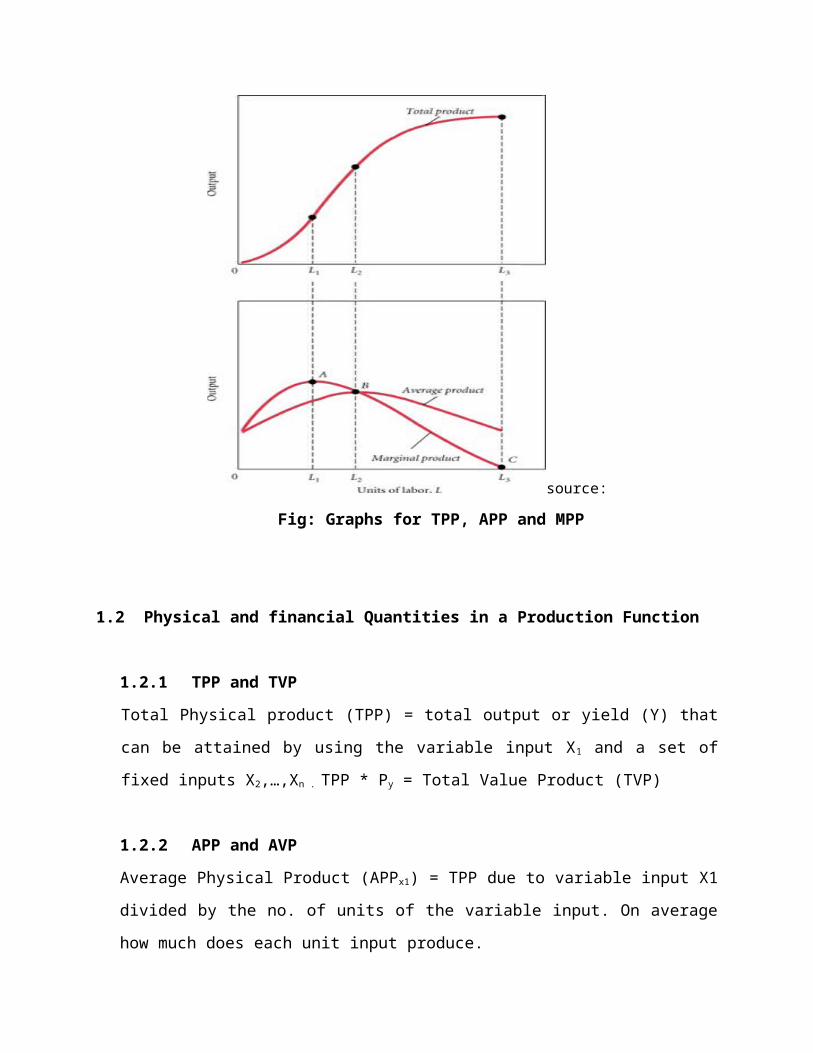
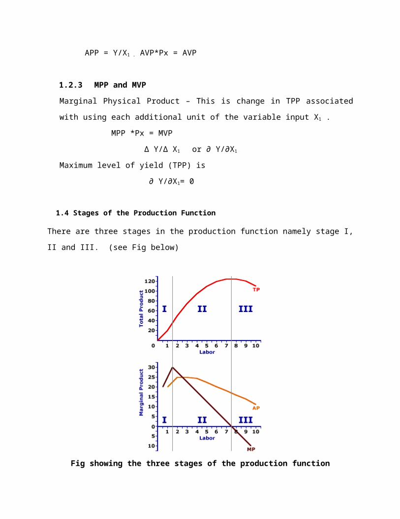
1.4 Stages of the Production Function

There are three stages in the production function namely stage I, II and III. (see Fig below)

Fig showing the three stages of the production function

1.4.1 Stage I

Short-run production Stage I arises due to increasing marginal returns. As more of the variable input is added to the fixed input, the marginal product of the variable input increases. This is directly illustrated by the slope of the marginal product curve, and because marginal product IS the slope of the total product curve, increasing marginal returns is also reflected in total

product. Stage 1 deals with increasing production for any input added. MPP is greater than APP. MPP is maximum. APP is still increasing

Consider these observations about the shapes and slopes of the three product curves in Stage I.

The total product curve has an increasing positive slope. In other words, the slope becomes steeper with each additional unit of variable input.

Marginal product is positive and the marginal product curve has a positive slope. The marginal product curve reaches a peak at the end of Stage I.

Average product is positive and the average product curve has a positive slope.

1.4.2 Stage II

In Stage II, short-run production is characterized by decreasing marginal returns. As more of the variable input is added to the fixed input, the marginal product of the variable input decreases. Most important of all, Stage II is driven by the law of diminishing marginal returns. The beginning of Stage II is the onset of the law of diminishing marginal returns.

The three product curves reveal the following patterns in Stage II.

The total product curve has a decreasing positive slope. In other words, the slope becomes flatter with each additional unit of variable input.

Marginal product is positive and the marginal product curve has a negative slope. The marginal product curve intersects the horizontal quantity axis at the end of Stage II.

Average product is positive and the average product curve at first has a positive slope, then it has a negative slope. The average product curve reaches a peak in the middle of Stage II. At this peak, average product is equal to marginal product.

The most profitable point of operation in stage 2 cannot be determined unless both resource and product prices are known

1.4.3 Stage III

The onset of Stage III results due to negative marginal returns. In this stage of short-run production, the law of diminishing marginal returns causes marginal product to decrease so much that it becomes negative.

Stage III production is most obvious for the marginal product curve, but is also indicated by the total product curve.

The total product curve has a negative slope. It has passed its peak and is heading down. Marginal product is negative and the marginal product curve has a negative slope. The

marginal product curve has intersected the horizontal axis and is moving down.

Average product remains positive but the average product curve has a negative slope.

1.5 Biological efficiency and economic efficiency

Biologists are concerned with the production response curve for fish as feed, seed, water

quality and other factors are varied

Economists are equally concerned with these response curves for establishing the cost

efficient level of production.

1.6 Elasticity of Response

Elasticity of response = relative change in Y/relative change in X1

(∂Y/y) (∂X1/X1) = (∂Y/ ∂X1) (Y/X1)

= MPP/APP

If you increase X1 how will output increase?

% ∆ in Y resulting from a 1% change in X1

1.7 Decision making rules

It is rational for a farmer to keep increasing input where TPP is increasing at an increasing rate

(where APP increases by increasing input). STAGE I

It is also not profitable to increase inputs that would decrease TPP (STAGE III). If TPP decreases

MPP becomes negative.

Rational area is between APP maximum and TPP maximum or between where MPP = APP and

where MPP = 0.

These three distinct stages of short-run production are not equally important. Stage I, and increasing marginal returns, is a great place to visit, but most firms move through it quickly. Because each variable input is increasingly more productive, firms employ as many as they can, as quickly as they can. Stage III, with negative marginal returns, is not particularly attractive to

firms. Production is less than it would be in Stage II, but the cost of production is greater due to the employment of the variable input. Not a lot of benefits are to be had with Stage III.

Stage II, with decreasing but positive marginal returns, provides a range of production that is suitable to most every firm. Although marginal product declines, additional employment of the variable input does add to total production. Even though production cost rises with additional employment, there are benefits to be gained from extra production. The trick is to balance the extra cost with the extra production.

As a matter of fact, because Stage II tends to be the choice of firms for short-run production, it is often referred to as the "economic region." Firms quickly move from Stage I to Stage II, and do all they can to avoid moving into Stage III. Firms can comfortably, and profitably, produce forever and ever in Stage II.

1.8 Profit Optimization

Where exactly in Stage II should you stop producing?

You need Px = Input price

Py = Output price

TPP * Py = Total Value Product (TVP)

MPP * Py = Value of Marginal Product (VMP)

APP * Py = Average Value Product

Economic Optimum is when Px = VMP

Price of input is equal to the additional revenue

realised from adding one more unit of input

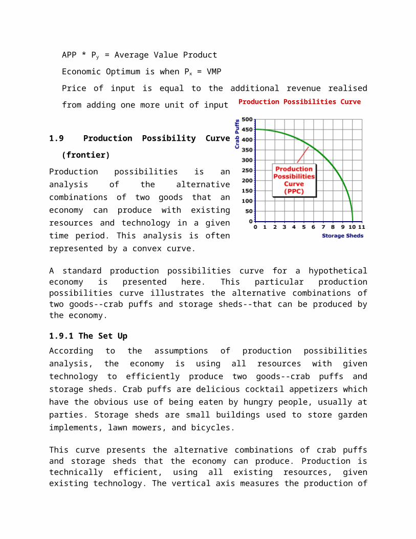
1.9 Production Possibility Curve (frontier)

Production possibilities is an analysis of the alternative combinations of two goods that an economy can

Production Possibilities Curve

produce with existing resources and technology in a given time period. This analysis is often represented by a convex curve.

A standard production possibilities curve for a hypothetical economy is presented here. This particular production possibilities curve illustrates the alternative combinations of two goods--crab puffs and storage sheds--that can be produced by the economy.

1.9.1 The Set Up

According to the assumptions of production possibilities analysis, the economy is using all resources with given technology to efficiently produce two goods--crab puffs and storage sheds. Crab puffs are delicious cocktail appetizers which have the obvious use of being eaten by hungry people, usually at parties. Storage sheds are small buildings used to store garden implements, lawn mowers, and bicycles.

This curve presents the alternative combinations of crab puffs and storage sheds that the economy can produce. Production is technically efficient, using all existing resources, given existing technology. The vertical axis measures the production of crab puffs and the horizontal axis measures the production of storage sheds.

1.9.2 Key Economic Concepts

As a introductory model of the economy, the production possibilities curve is commonly used to illustrate basic economic concepts, including full employment, unemployment, opportunity cost, economic growth, and investment.

Opportunity Cost: This is indicated by the negative slope of the production possibilities curve (or frontier). As more storage sheds are produced, fewer crab puffs are produced. This reduction in the production of crab puffs is the opportunity cost of storage shed production.

Full Employment: This is indicated by producing on the production possibilities curve. The curve indicates the maximum production of crab puffs and storage sheds obtained with existing technology, given that all available resources are engaged in production.

Unemployment: This is indicated by producing inside the production possibilities curve. If some available resources are not engaged in production, then the economy is not achieving maximum production.

Economic Growth: This is indicated by an outward shift of the production possibilities curve, which is achieved by relaxing the assumptions of fixed resources and technology or by increasing the quantity or quality of resources. With economic growth more of both goods, crab puffs and storage sheds, can be produced.

Investment: This is indicated by a tradeoff between the production of consumption goods (crab puffs) and capital goods (storage sheds). Investment results if society moves

along the production possibilities curve, producing more capital goods and fewer consumption goods.

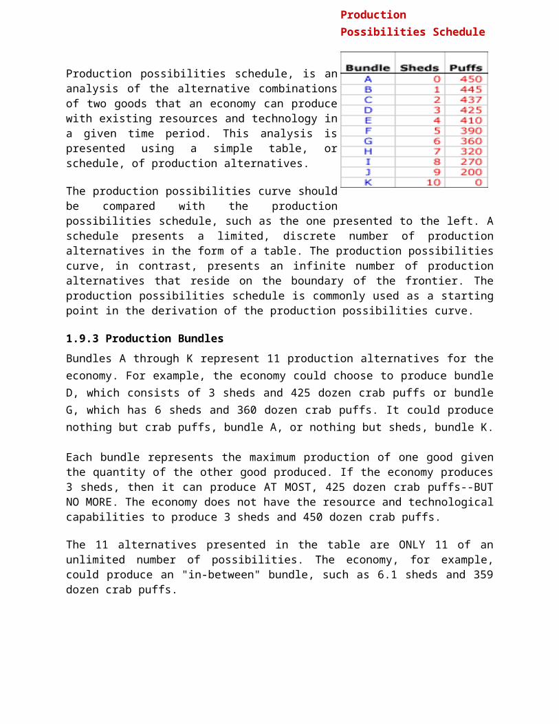
Production possibilities schedule, is an analysis of the alternative combinations of two goods that an economy can produce with existing resources and technology in a given time period. This analysis is presented using a simple table, or schedule, of production alternatives.

The production possibilities curve should be compared with the production possibilities schedule, such as the one presented to the left. A schedule presents a limited, discrete number of production alternatives in the form of a table. The production possibilities curve, in contrast, presents an infinite number of production alternatives that reside on the boundary of the frontier. The production possibilities schedule is commonly used as a starting point in the derivation of the production possibilities curve.

1.9.3 Production Bundles

Bundles A through K represent 11 production alternatives for the economy. For example, the economy could choose to produce bundle D, which consists of 3 sheds and 425 dozen crab puffs or bundle G, which has 6 sheds and 360 dozen crab puffs. It could produce nothing but crab puffs, bundle A, or nothing but sheds, bundle K.

Each bundle represents the maximum production of one good given the quantity of the other good produced. If the economy produces 3 sheds, then it can produce AT MOST, 425 dozen crab puffs--BUT NO MORE. The economy does not have the resource and technological capabilities to produce 3 sheds and 450 dozen crab puffs.

The 11 alternatives presented in the table are ONLY 11 of an unlimited number of possibilities. The economy, for example, could produce an "in-between" bundle, such as 6.1 sheds and 359 dozen crab puffs.

1.9.4 A Tradeoff

Moving down the alphabet from bundle A to bundle K reveals an important pattern. The number of storage sheds produced increases from 0 to 10, but the quantity of crab puffs produced decreases from 450 dozen to 0.

In other words, there is a tradeoff between the production of sheds and crab puffs. As more sheds are produced, fewer crab puffs are produced.

Production Possibilities Schedule

The reason for this tradeoff can be traced to the basic assumptions underlying production possibilities analysis, especially fixed resources. Because resources are fixed, producing more of one good necessarily means producing less of the other. That is, to produce more sheds, the economy must forego the production of crab puffs.

1.9.5 Enter Opportunity Cost

This tradeoff indicates opportunity cost. Opportunity cost is the highest valued alternative foregone in the pursuit of an activity. The opportunity cost of producing storage sheds is the foregone production of crab puffs.

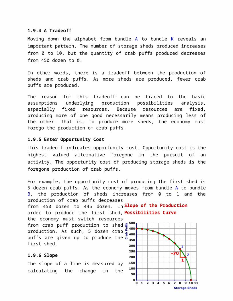
For example, the opportunity cost of producing the first shed is 5 dozen crab puffs. As the economy moves from bundle A to bundle B, the production of sheds increases from 0 to 1 and the production of crab puffs decreases from 450 dozen to 445 dozen. In order to produce the first shed, the economy must switch resources from crab puff production to shed production. As such, 5 dozen crab puffs are given up to produce the first shed.

1.9.6 Slope

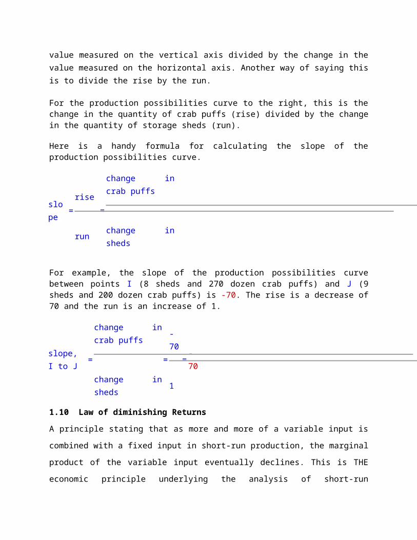
The slope of a line is measured by calculating the change in the value measured on the vertical axis divided by the change in the value measured on the horizontal axis. Another way of saying this is to divide the rise by the run.

For the production possibilities curve to the right, this is the change in the quantity of crab puffs (rise) divided by the change in the quantity of storage sheds (run).

Here is a handy formula for calculating the slope of the production possibilities curve.

slope =

rise

run

=

change in crab puffs

change in sheds

For example, the slope of the production possibilities curve between points I (8 sheds and 270 dozen crab puffs) and J (9 sheds and 200 dozen crab puffs) is -70. The rise is a decrease of 70 and the run is an increase of 1.

slope, I to J = change in crab puffs = -70 = -70

Slope of the Production Possibilities Curve

change in sheds1

1.10 Law of diminishing Returns

A principle stating that as more and more of a variable input is combined with a fixed input in

short-run production, the marginal product of the variable input eventually declines. This is THE

economic principle underlying the analysis of short-run production for a firm. Among a host of

other things, it offers an explanation for the upward-sloping market supply curve. How does the

law of diminishing marginal returns help us understand supply? The law of supply and the

upward-sloping supply curve indicate that a firm needs to receive higher prices to produce and

sell larger quantities.

2.0 Learning Activities

Tutorials, Assignments and Quizzes

3.0 Summary of Topic

In this topic you have learnt the concept of production and the relationship between inputs and

outputs. You also learnt that maximum production does not necessarily mean maximum profits

(economic and biological efficiency). In order to maximize profits we need to equate Marginal

Revenue to Marginal Cost (additional revenue should be equal to additional cost of producing

it)

4.0 Further Reading Materials

Jolly, C.M., and Clonts, H. A. (1993). Economics of Aquaculture. Food Products Press, an

Imprint of the Hearth Press, Inc.,

Chiang, Alpha C. (1984) Fundamental Methods of Mathematical Economics, third edition,

McGraw-Hill.

5.0 Useful Links

http://en.wikipedia.org/wiki/Production_function

Topic 2: LINEAR PROGRAMMING

Learning Outcomes

Upon completion of this lesson you will be able to;

Determine optimal combination of inputs to maximize profit or minimize cost.

Key Terms: Linear Programming, Optimization, linear Objective Function

1 Definition of Linear Programming

Linear programming (LP) is a mathematical method for determining a way to achieve the best

outcome (such as maximum profit or lowest cost) in a given mathematical model for some list

of requirements represented as linear equations. This entails there is a linear relationship

between inputs and outputs.

More formally, linear programming is a technique for the optimization of a linear objective

function, subject to linear equality and linear inequality constraints

2 Use of LP

Linear programming is a considerable field of optimization for several reasons. Although the

modern management issues are ever-changing, most companies would like to maximize profits

or minimize costs with limited resources. Therefore, many issues can be characterized as linear

programming problems. Linear programming can be applied to various fields of study. It is used

most extensively in business and economics, but can also be utilized for some engineering

problems. Industries that use linear programming models include transportation, energy,

telecommunications, and manufacturing. It has proved useful in modeling diverse types of

problems in planning, routing, scheduling, assignment, and design.

3 Basic Assumptions of LP

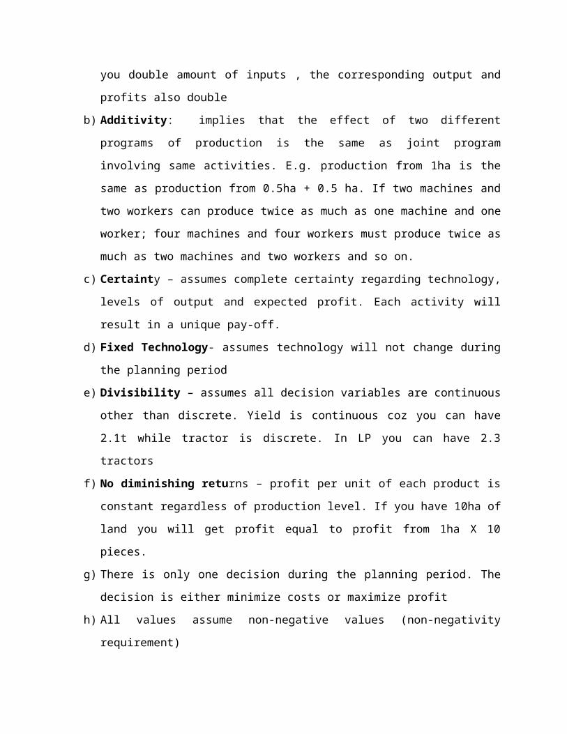
a) Linearity: implies proportionality (straight line) and additivity among the relevant

variables. Proportionality in economic theory is known as constant returns which means

if you double amount of inputs , the corresponding output and profits also double

b) Additivity: implies that the effect of two different programs of production is the same

as joint program involving same activities. E.g. production from 1ha is the same as

production from 0.5ha + 0.5 ha. If two machines and two workers can produce twice as

much as one machine and one worker; four machines and four workers must produce

twice as much as two machines and two workers and so on.

c) Certainty – assumes complete certainty regarding technology, levels of output and

expected profit. Each activity will result in a unique pay-off.

d) Fixed Technology- assumes technology will not change during the planning period

e) Divisibility – assumes all decision variables are continuous other than discrete. Yield is

continuous coz you can have 2.1t while tractor is discrete. In LP you can have 2.3

tractors

f) No diminishing returns – profit per unit of each product is constant regardless of

production level. If you have 10ha of land you will get profit equal to profit from 1ha X

10 pieces.

g) There is only one decision during the planning period. The decision is either minimize

costs or maximize profit

h) All values assume non-negative values (non-negativity requirement)

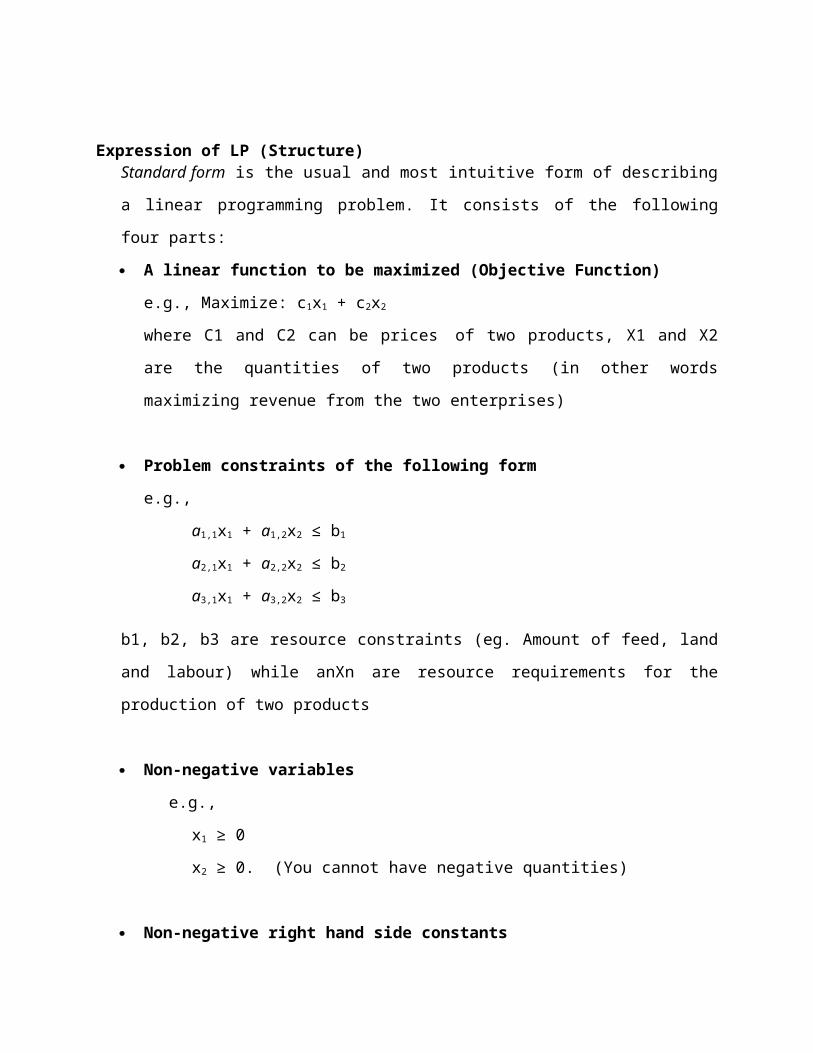
Expression of LP (Structure)Standard form is the usual and most intuitive form of describing a linear programming

problem. It consists of the following four parts:

A linear function to be maximized (Objective Function)

e.g., Maximize: c1x1 + c2x2

where C1 and C2 can be prices of two products, X1 and X2 are the quantities of two

products (in other words maximizing revenue from the two enterprises)

Problem constraints of the following form

e.g.,

a1,1x1 + a1,2x2 ≤ b1

a2,1x1 + a2,2x2 ≤ b2

a3,1x1 + a3,2x2 ≤ b3

b1, b2, b3 are resource constraints (eg. Amount of feed, land and labour) while anXn are

resource requirements for the production of two products

Non-negative variables

e.g.,

x1 ≥ 0

x2 ≥ 0. (You cannot have negative quantities)

Non-negative right hand side constants

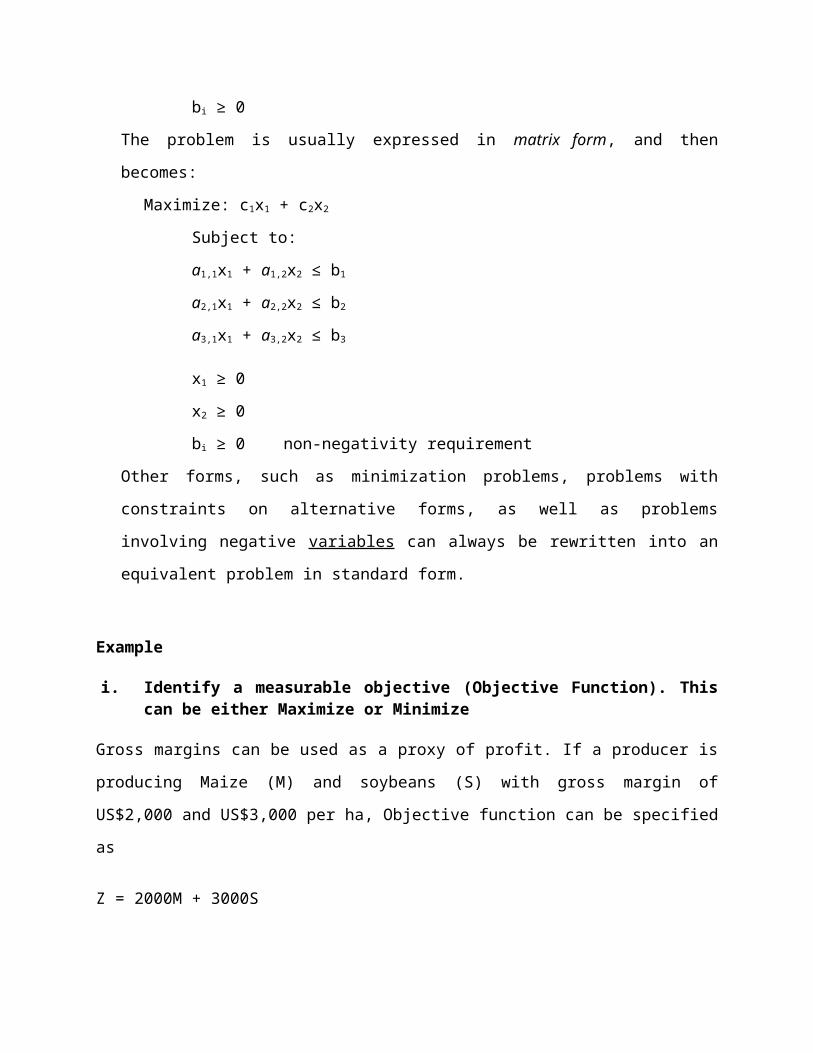
bi ≥ 0

The problem is usually expressed in matrix form, and then becomes:

Maximize: c1x1 + c2x2

Subject to:

a1,1x1 + a1,2x2 ≤ b1

a2,1x1 + a2,2x2 ≤ b2

a3,1x1 + a3,2x2 ≤ b3

x1 ≥ 0

x2 ≥ 0

bi ≥ 0 non-negativity requirement

Other forms, such as minimization problems, problems with constraints on alternative

forms, as well as problems involving negative variables can always be rewritten into an

equivalent problem in standard form.

Example

i. Identify a measurable objective (Objective Function). This can be either Maximize or Minimize

Gross margins can be used as a proxy of profit. If a producer is producing Maize (M) and

soybeans (S) with gross margin of US$2,000 and US$3,000 per ha, Objective function can be

specified as

Z = 2000M + 3000S

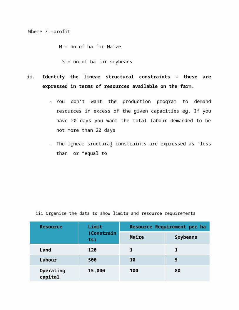
Where Z =profit

M = no of ha for Maize

S = no of ha for soybeans

ii. Identify the linear structural constraints – these are expressed in terms of resources

available on the farm.

- You don’t want the production program to demand resources in excess of the

given capacities eg. If you have 20 days you want the total labour demanded to

be not more than 20 days

- The linear sructural constraints are expressed as “less than” or “equal to”

iii Organize the data to show limits and resource requirements

Resource Limit (Constraints)

Resource Requirement per ha

Maize Soybeans

Land 120 1 1

Labour 500 10 5

Operating capital 15,000 100 80

Gross Margin 1200 950

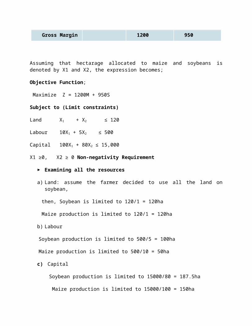
Assuming that hectarage allocated to maize and soybeans is denoted by X1 and X2, the expression becomes;

Objective Function;

Maximize Z = 1200M + 950S

Subject to (Limit constraints)

Land X1 + X2 ≤ 120

Labour 10X1 + 5X2 ≤ 500

Capital 100X1 + 80X2 ≤ 15,000

X1 ≥0, X2 ≥ 0 Non-negativity Requirement

Examining all the resources

a) Land: assume the farmer decided to use all the land on soybean,

then, Soybean is limited to 120/1 = 120ha

Maize production is limited to 120/1 = 120ha

b) Labour

Soybean production is limited to 500/5 = 100ha

Maize production is limited to 500/10 = 50ha

c) Capital

Soybean production is limited to 15000/80 = 187.5ha

Maize production is limited to 15000/100 = 150ha

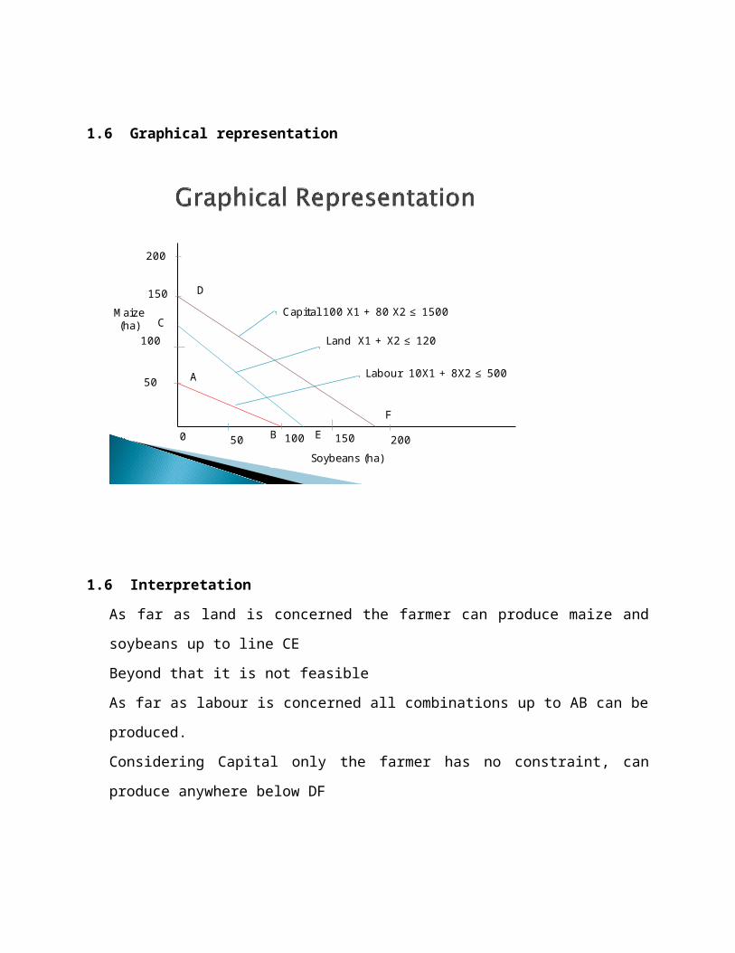
1.6 Graphical representation

Maize (ha)

Soybeans (ha)0 50 100 150 200

50

100

150

200

A

B

C

E

D

F

Capital 100 X1 + 80 X2 ≤ 1500

Labour 10X1 + 8X2 ≤ 500

Land X1 + X2 ≤ 120

1.6 Interpretation

As far as land is concerned the farmer can produce maize and soybeans up to line CE

Beyond that it is not feasible

As far as labour is concerned all combinations up to AB can be produced.

Considering Capital only the farmer has no constraint, can produce anywhere below DF

The producer has to produce using a combination of resources. The production will be

constrained by the least available resource.

ABO is the production possibility curve

1.7 Existence of optimal solutions

Geometrically, the linear constraints define a convex polytope, which is called the feasible

region. A linear function is a convex function, which implies that every local minimum is a

global minimum; similarly, a linear function is a concave function, which implies that every

local maximum is a global maximum.

Optimal solution need not exist, for two reasons. First, if two constraints are inconsistent,

then no feasible solution exists: For instance, the constraints x ≥ 2 and x ≤ 1 cannot be

satisfied jointly; in this case, we say that the LP is infeasible. Second, when the polytope is

unbounded in the direction of the gradient of the objective function (where the gradient of

the objective function is the vector of the coeffients of the objective function), then no

optimal value is attained.

Fig 1: showing feasible region given a number of constraints

Learning Activities

Assignments on solving maximization and minimization problems

Summary of Topic

In this topic you have learnt the Linear programming Technique in solving profit maximization

and cost minimization problems given limited resources. You also learnt that you can have dual

solution in Linear Programming

Further Reading Materials

Bernd Gärtner, Jiří Matoušek (2006). Understanding and Using Linear Programming,

Berlin: Springer. ISBN 3-540-30697-8 (elementary introduction for mathematicians and

computer scientists)

Dmitris Alevras and Manfred W. Padberg, Linear Optimization and Extensions:

Problems and Extensions, Universitext, Springer-Verlag, 2001. (Problems from Padberg

with solutions.)

A. Bachem and W. Kern. Linear Programming Duality: An Introduction to Oriented

Matroids. Universitext. Springer-Verlag, 1992. (Combinatorial)

J. E. Beasley, editor. Advances in Linear and Integer Programing. Oxford Science, 1996.

(Collection of surveys)

Useful Links

http://en.wikipedia.org/wiki/Linear_programming

http://wiki.mcs.anl.gov/NEOS/index.php/

Topic 3: Theory of demand

Learning Outcomes

Upon completion of this lesson you will be able to;

Explain the theory of demand Analyze the demand Apply the theory of demand in marketing of fish and fish products

Key Terms: Demand, Supply, Utility, Law of Demand

1.0 Introduction to Theory of Demand

The theory of supply and demand is one of the fundamental theories of economics and is the foundation upon which many other more elaborate economic models and theories are based. The theory is a valuable tool that is used by schools of economics in order to explain the workings of a market economy, since supply and demand are crucial elements that directly affect resource allocation.

By definition, supply is the amount of product that a producer is willing and able to sell at a specified price, while demand is the amount of product that a buyer is willing and able to buy at a specified price. Thus, the supply and demand model shows the relationships between a product’s accessibility and the interest shown in it. Unlike with general equilibrium models, however, this model does not define the attributes that are responsible for supply schedules.

Economic theory is based on developing supply and demand models and then factoring in whatever elements might cause disruption to their smooth flow. One limitation of the theory, though, is its simplistic approach in assuming perfectly competitive markets where no single group of buyers or sellers has the power to affect pricing. Whereas effective when accurate, the theory falters when up against actual scenarios that are not so equal and that, therefore, require a more intricate degree of analysis.

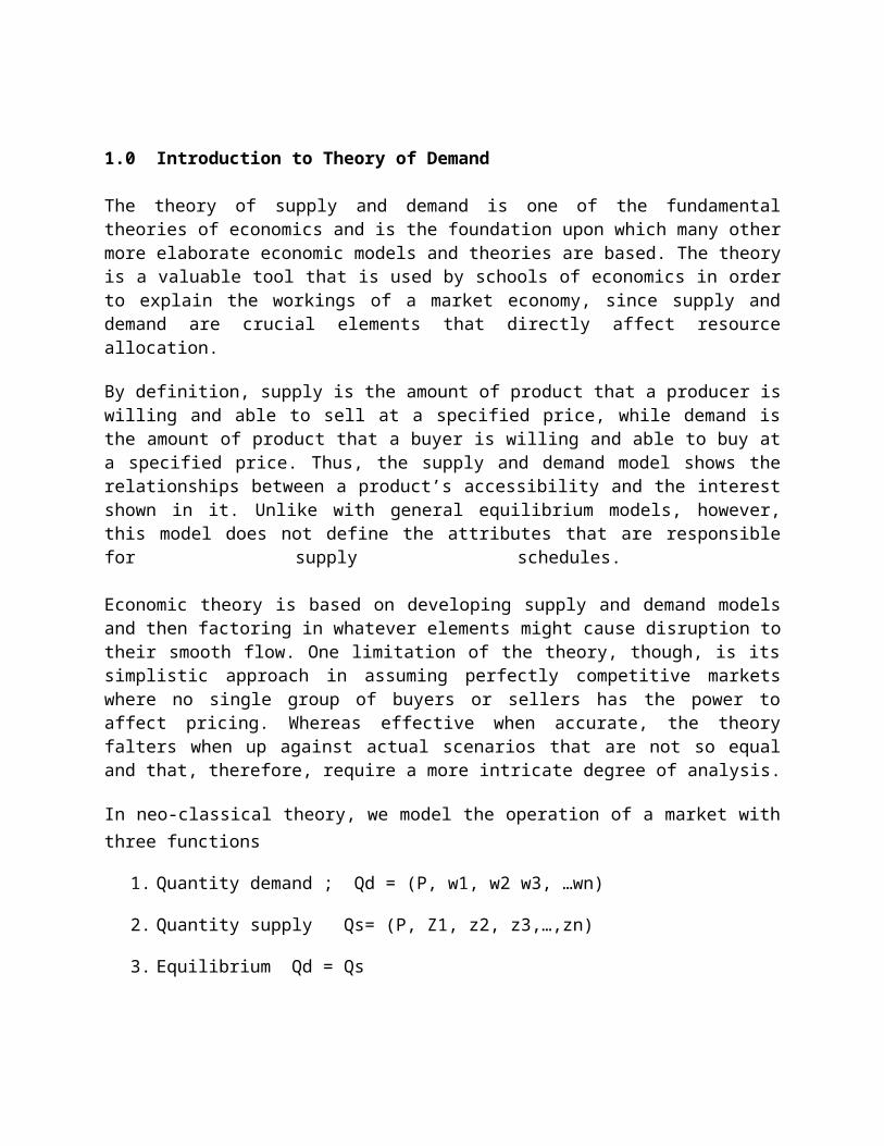
In neo-classical theory, we model the operation of a market with three functions

1. Quantity demand ; Qd = (P, w1, w2 w3, …wn)

2. Quantity supply Qs= (P, Z1, z2, z3,…,zn)

3. Equilibrium Qd = Qs

Q

P S

D

Fig showing market equilibrium

This is based on theory of consumer behaviour – how do you expect the consumers to behave

in the market. The theory states that consumers purchase more when the prices are low and

less as the prices increases. Consumers purchase what gives them the greatest overall level of

satisfaction.

1.1 Approaches to analyzing the theory of Demand

These are Cardinalist approach –cardinal theory and Ordinalist approach – ordinal theory

1.1.1 Assumptions of the approaches

1. Consumer is rational, i.e. given two products Q1 and Q2 which give the same

satisfaction, the rational consumer will only look at price.

2. Consumer’s objective is to maximize satisfaction

Given U = U(Q)

∂u/ ∂Q = 0 first order stationery point

∂2u/∂Q2 < 0 utility is maximized

This implies that given the prices and income, the consumer plans how to spend the money to

get maximum satisfaction. This is called the Axiom of utility satisfaction

3. It is assumed that consumers have unbounded rationality- have full knowledge of the

market in terms of prices of goods and services available and his/her income. It is also

expected that the consumers make a rational choice, ie. to maximize utility a consumer

must compare utilities derived from various baskets of goods and services with which

their income can buy.

4. Monotonicity – more is better than less. That is consumers would prefer to buy more

with the disposable income that they have.

5. Transitivity – if you have three goods q1, q2 and q3; if you prefer q1 to q2 and if you

prefer q2 to q3 then you must prefer q1 to q3

6. Completeness – if you have q1 and q2, you either prefer q1 to q2 or you prefer q2 to q1

i.e. q1 I q2 ( q1 is indifferent from q2)

Example:

Max U = u (q1 q2) ………………….(a)

Subject to 5q1 + 2q2 = 1 ……….(b)

5q1 + 2q2 = 1…………………………..(c)

q2 = 1-5q1……………………………….(d)

Substituting q2 in (c)

U = 2q1(1-5q1)

1.1.2 Cardinal Approach

Utility is a measure of personal satisfaction derived from owning and using goods and services.

Alfred Marshall, Stanley Jevons and Leon Walras developed this. They made two assumptions in

Cardinal approach;

a) Utility can be measured quantitatively like weight and each commodity has its own

unique utility

• Each consumer is in a position to assign the amount of utility he will get from consuming

different commodities or combination of commodities (assign a figure). This assumption

means the consumer has cardinal measure of utility. 1 unit of utility is called util. People

who believe in this theory are called cardinalist. Cardinal utility is also called Utility

Analysis

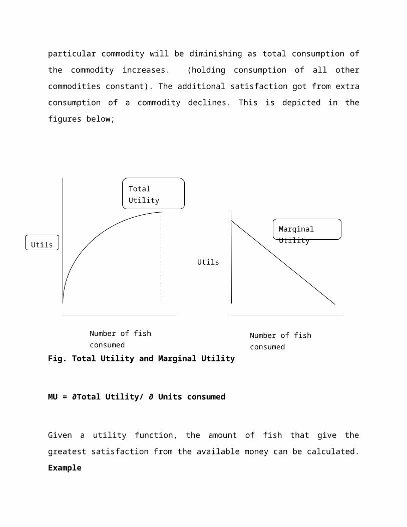
Of fundamental importance in theory of consumer behaviour is the law of diminishing marginal

utility. It states that utility that any individual or household derives from successive units of

particular commodity will be diminishing as total consumption of the commodity increases.

(holding consumption of all other commodities constant). The additional satisfaction got from

extra consumption of a commodity declines. This is depicted in the figures below;

Fig. Total Utility and Marginal Utility

Total Utility

Marginal Utility

Utils

Utils

Number of fish consumed Number of fish consumed

MU = ∂Total Utility/ ∂ Units consumed

Given a utility function, the amount of fish that give the greatest satisfaction from the available

money can be calculated.

Example

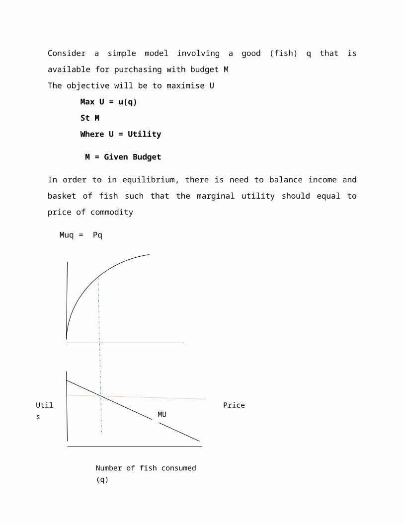
Consider a simple model involving a good (fish) q that is available for purchasing with budget M

The objective will be to maximise U

Max U = u(q)

St M

Where U = Utility

M = Given Budget

In order to in equilibrium, there is need to balance income and basket of fish such that the

marginal utility should equal to price of commodity

Muq = Pq

PriceMU

Utils

Number of fish consumed (q)

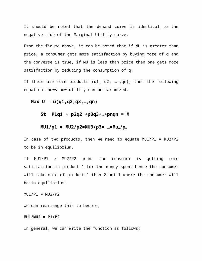
It should be noted that the demand curve is identical to the negative side of the Marginal Utility

curve.

From the figure above, it can be noted that if MU is greater than price, a consumer gets more

satisfaction by buying more of q and the converse is true, if MU is less than price then one gets

more satisfaction by reducing the consumption of q.

If there are more products (q1, q2, ….,qn), then the following equation shows how utility can be

maximized.

Max U = u(q1,q2,q3,…,qn)

St P1q1 + p2q2 +p3q3+…+pnqn = M

MU1/p1 = MU2/p2=MU3/p3= …=Mun/pn

In case of two products, then we need to equate MU1/P1 = MU2/P2 to be in equilibrium.

If MU1/P1 > MU2/P2 means the consumer is getting more satisfaction in product 1 for the

money spent hence the consumer will take more of product 1 than 2 until where the consumer

will be in equilibrium.

MU1/P1 = MU2/P2

we can rearrange this to become;

MU1/MU2 = P1/P2

In general, we can write the function as follows;

U = u (x)

Subject to M (budget)

Max U = P1X1

∂u/ ∂x = P1

We know that ∂u/ ∂x = Mux

Therefore P1 = MUx

Example

Max U = 2XY

St 4X + Y = 1

We solve this by using Lagrangean multiplier λ ( Lambda)

1 – 4X + Y = 0

λ (1 – 4X + Y) = 0

L = 2XY + λ (1 – 4X + Y)

dL/dX = 2Y – 4 λ = 0

2Y = 4λ

Y = 2λ

dL/dY = 2X –λ = 0

2x = λ

X = 0.5λ

dL/dλ = 0 (λ is a constant)

4x + Y = 1

4 (0.5λ) + 2λ = 1

2λ + 2λ = 1

λ = ¼

Therefore Y = 1/2

X = ½ * ¼ = 1/8

U = 2XY

= 2 (1/8) * ½

= ½

If budget changes from original M and increase by 1 then U will increase by λ to maintain Px = Mux

M + 1 = U + λ

1.1.2 Criticisms of cardinal approach

Cardinal approach to analysing demand has the following criticisms;

• It is impossible to attach an objective value to utility. The level of satisfaction differs between individuals

• λ being constant is unrealistic (constant marginal utility of money does not hold) – when income changes the prices changes as well therefore λ is not constant

1.2 Ordinal Approach

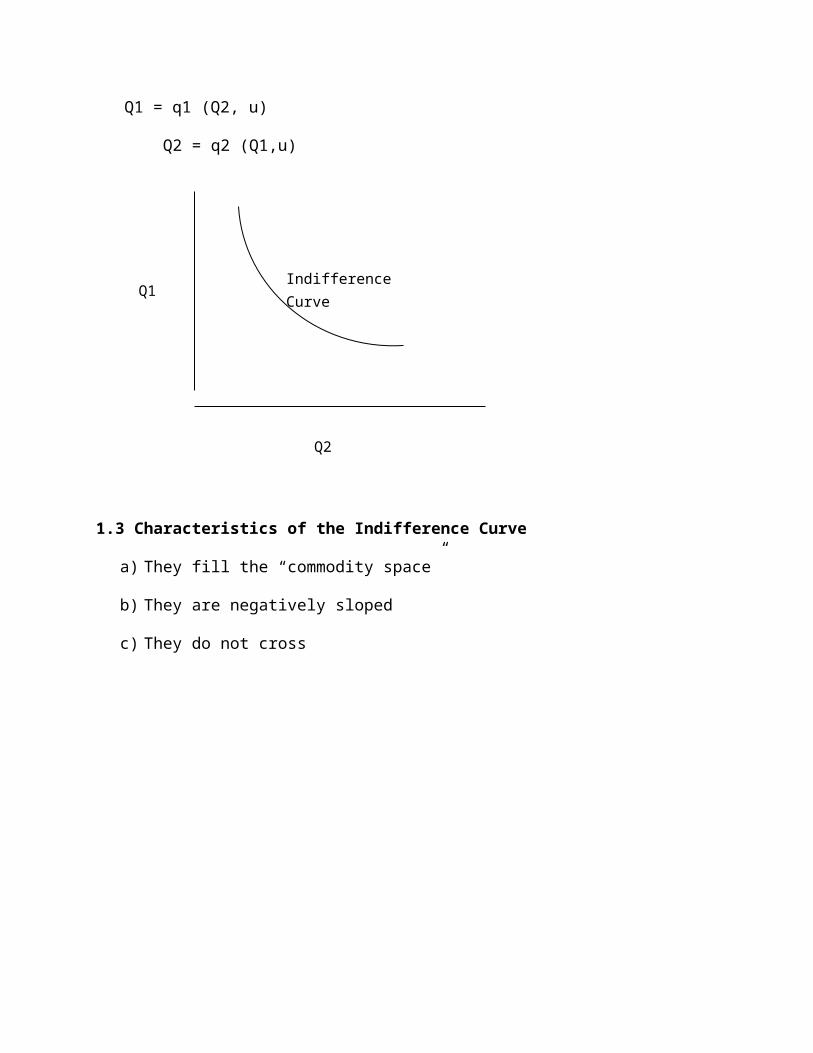
The Ordinal approach considers indifference curve which is a locus of consumption bundles that yield the consumer an identical amount of satisfaction. The Ordinal approach assumes that a 2 product world such that

U = u (Q1,Q2)

Q1 = q1 (Q2, u)

Q2 = q2 (Q1,u)

Q1

Q2

Indifference Curve

1.3 Characteristics of the Indifference Curve

a) They fill the “commodity space”

b) They are negatively sloped

c) They do not cross

Q1

Q2

Q1

Q2

U2

U1

U2

U1C

A

B

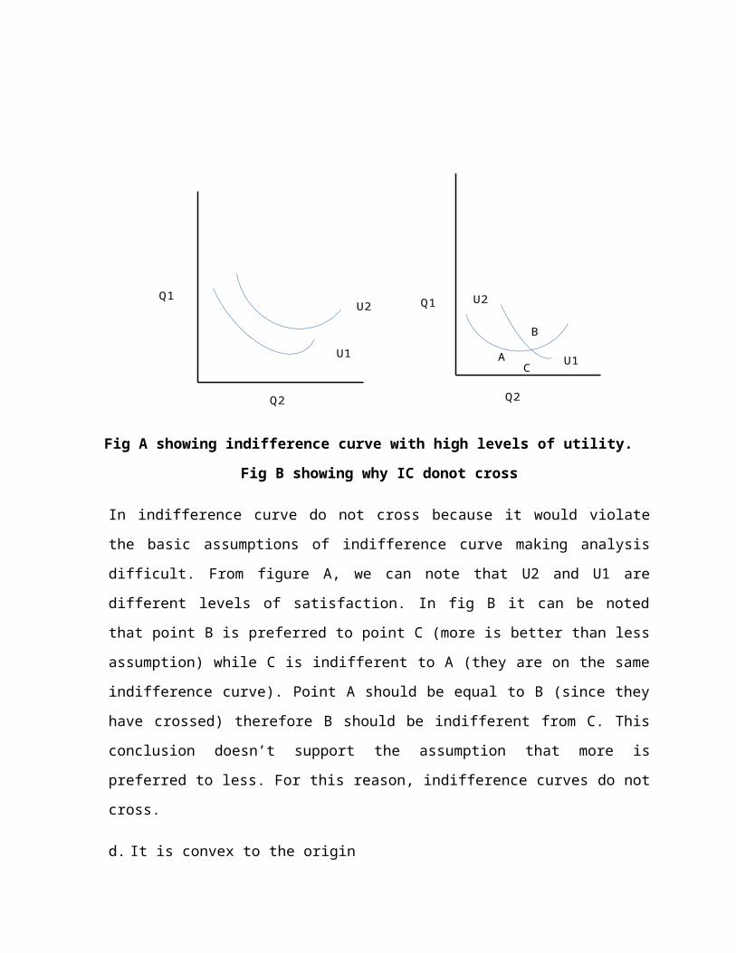
Fig A showing indifference curve with high levels of utility. Fig B showing why IC donot cross

In indifference curve do not cross because it would violate the basic assumptions of

indifference curve making analysis difficult. From figure A, we can note that U2 and U1 are

different levels of satisfaction. In fig B it can be noted that point B is preferred to point C

(more is better than less assumption) while C is indifferent to A (they are on the same

indifference curve). Point A should be equal to B (since they have crossed) therefore B

should be indifferent from C. This conclusion doesn’t support the assumption that more is

preferred to less. For this reason, indifference curves do not cross.

d. It is convex to the origin

1.4 Assumptions to indifferent analysis

a) Rationality – consumers are rational in their decision making

b) Ordinal utility – you can rank products according to how you feel

c) Marginal rate of commodity substitution – when you increase the consumption of one

commodity, you must decrease the consumption of the other.

d) Total utility depends on goods and services consumed

e) Consistency and transitivity.

1.5 Consumer Equilibrium

A consumer is said to be in equilibrium when there is a balance between additional utility and

the prices of commodities. Therefore the level of income will determine the bundles of

commodities that a consumer will get. The budget line is a line that shows the combination of

quantities of two products that can be bought by a given level of income.

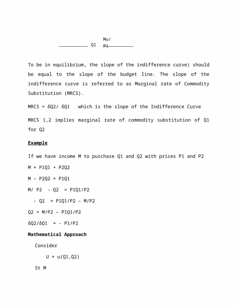
To be in equilibrium, the slope of the indifference curve) should be equal to the slope of the

budget line. The slope of the indifference curve is referred to as Marginal rate of Commodity

Substitution (MRCS).

MRCS = δQ2/ δQ1 which is the slope of the Indifference Curve

Q1

Q2

Mu/P1

Mu/P2

U

δQ2/δQ1 = - P1/P2

MRCS 1,2 implies marginal rate of commodity substitution of Q1 for Q2

Example

If we have income M to purchase Q1 and Q2 with prices P1 and P2

M = P1Q1 + P2Q2

M – P2Q2 = P1Q1

M/ P2 - Q2 = P1Q1/P2

- Q2 = P1Q1/P2 – M/P2

Q2 = M/P2 – P1Q1/P2

δQ2/δQ1 = - P1/P2

Mathematical Approach

Consider

U = u(Q1,Q2)

St M

P1Q1 + P2Q2 = M

Recall that MU1/P1 = MU2/P2

And note that the budget M can be expressed as

M = ∑PiQi

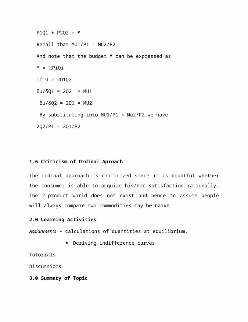
If U = 2Q1Q2

δu/δQ1 = 2Q2 = MU1

δu/δQ2 = 2Q1 = MU2

By substituting into MU1/P1 = Mu2/P2 we have

2Q2/P1 = 2Q1/P2

1.6 Criticism of Ordinal Aproach

The ordinal approach is criticized since it is doubtful whether the consumer is able to acquire

his/her satisfaction rationally. The 2-product world does not exist and hence to assume people

will always compare two commodities may be naïve.

2.0 Learning Activities

Assignments – calculations of quantities at equilibrium.

Deriving indifference curves

Tutorials

Discussions

3.0 Summary of Topic

In this lesson you have learnt the theory of demand. You have learnt the two approaches to studying demand. That is cardinal and ordinal approach. The cardinal approach assumes utlty can be quantified while ordinal approach assumes a 2-commodity world and that when consumption of one commodity increases the utility of the other decreases. It can be noted that both approaches had their assumptions and their weaknesses. The equilibrium is attained when Mu = Px

4.0 Further Reading Materials Goodwin, N, Nelson, J; Ackerman, F & Weissskopf, T: Microeconomics in Context 2d ed.

Sharpe 2009 ISBN 9780765623010 Colander, David. Microeconomics. McGraw-Hill Paperback, 7th Edition: 2008.

Perloff, Jeffrey M. Microeconomics: Theory and Applications with Calculus. Pearson - Addison Wesley, 1st Edition: 2007

5.0 Useful Links

http://en.wikipedia.org/wiki/Supply_and_demand

Topic 4: Market Structure, Conduct and Performance

Learning Outcomes

Upon completion of this lesson you will be able to;

4 Describe the link among market structure, conduct and performance.

5 Analyze the market efficiency of different fish and fish products

6 Apply knowledge of market structure, conduct and performance in the marketing of fish and fish products

Key Terms: competitive market, monopoly, oligopoly, market efficiency

1.0 Introduction

The Market Structure consists of the relatively stable features of the market environment that

influence rivalry among the buyers and sellers operating within this market. They are the

oorganizational characteristics of a market. These are the ones which influence the

relationship among buyers, sellers and between buyers and sellers. Therefore they influence

competition and pricing activities within the market

The main elements that influence market structure are, seller concentration, product

differentiation, barriers to entry, barriers to exit, buyer concentration, and the growth rate of

market demand. Other elements of market structure exist, but they are usually unstable and

therefore ignored either because they can’t be measured or because they are hard to observe.

2.0 Elements of Market Structure

2.1 Seller Concentration

It refers to the number and size distribution of firms in the market. The most widely used device

is determining seller concentration is the Concentration Ratio. To compute the concentration

ratio, the firms are ranked in order of size “usually measured in terms of sale”, starting from the

largest in the industry at the top and going down to the smallest firm at the bottom.

Concentration ratios are usually given for the largest 4, largest 8, and sometimes the largest 20

firms. Usually industries that are highly concentrated in one advanced economy tend to be

highly concentrated in another.

2.2 Buyer concentration:

This is the number of buyers and sellers in a market. Buyer concentration is as equally

important as seller concentration, especially in markets with a few buyers. Ideally it is expected

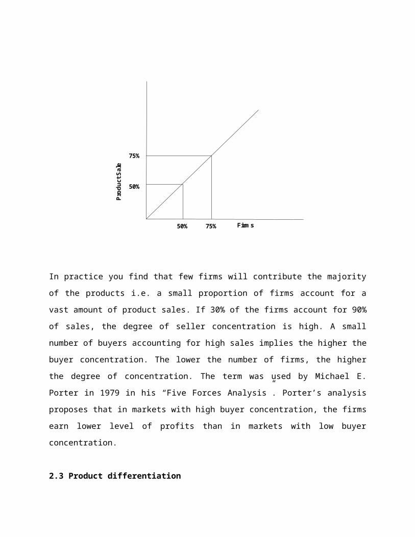
that 50% of firms in the market contribute 50% of the volume of product. The fig below show

an ideal market

50%

50% 75%

75%

Prod

uct S

ale

Firms

In practice you find that few firms will contribute the majority of the products i.e. a small

proportion of firms account for a vast amount of product sales. If 30% of the firms account for

90% of sales, the degree of seller concentration is high. A small number of buyers accounting

for high sales implies the higher the buyer concentration. The lower the number of firms, the

higher the degree of concentration. The term was used by Michael E. Porter in 1979 in his “Five

Forces Analysis”. Porter’s analysis proposes that in markets with high buyer concentration, the

firms earn lower level of profits than in markets with low buyer concentration.

2.3 Product differentiation

This implies the differentiation or distinguishing a product from the products of other

competing firms. Differentiation of products along key features and minor details is an

important strategy for firms to defend their price from leveling down to marginal cost. Whether

the products sold are homogenous of there are differences in quality, design and packaging

(which might influence consumer preference). One looks at the differences in the product. The

wider the differences, the higher the degree of product differentiation, the lesser the

competition. This is inefficient market system.Consumers get best services if there is

competition

2.3.1 Horizontal differentiation

When products are different according to features that can't be ordered in an objective way, or

in other words, at the same price, some consumers would prefer the product while others

would prefer a different substitute Horizontal differentiation can be differentiation in colors

(different color version for the same good), in styles (e.g. modern/antique), or in tastes. A

typical example is the ice cream offered in different tastes. Chocolate is not better than Mango.

2.3.2 Vertical differentiation

Vertical differentiation occurs in a market where the several goods that are present can be

ordered according to their objective quality from the highest to the lowest. It's possible to say

in this case that one good is "better" than another.

2.3.3 Mixed differentiation

Certain markets are characterized by both horizontal and vertical differentiation. For instance,

apparel, and shoes have a rich combination of shapes, colors, materials, and appropriateness to

social events. In such markets, the differences in colors or shapes are horizontal differentiation,

while the quality of the materials is usually perceived as vertical differentiation.

2.4 Barriers to entry

A set of economic forces that create a disadvantage to new competitors attempting to enter

the market. That is, how difficult is it for new firms to enter the market. These forces could be

government regulation such as IP rights, or patent, or they could be large economies of scale in

a specific industry, or high sunk costs required entering the market. Sometimes firms within a

specific industry adopt certain pricing strategies to create barriers to entry, one of the most

widely adopted strategy is “Limit Pricing” by lowering prices to a level that would force any new

entrants to operate at a loss, this strategy is especially effective when the existing firms have a

cost advantage over potential entrants. Reasons why some monopolies exist are;

i. Legal restrictions – by law preventing other firms from operating in some sectors

ii. Patents- to encourage innovativeness government may give exclusive production rights

it has invented a product

iii. Control of scarce resource – Some products use materials and the firm that gets hold of

that resource controls the production.

iv. Cost advantage of large firms (natural monopoly)- Cost of production of large firms may

be lower than that of new firms. Large firms can manage to reduce prices to levels

which new firms cannot manage. (Price squeeze)

v. Heavy investment ; if an industry require heavy industry only few would manage

creating a monopoly

i. Small market – the market may be too small to have more firms

2.5 Barriers to exit

A set of economics forces that influence the firm’s decision of exiting the market, such forces

make it cheaper for the existing firm to stay in the market than to exit the market. Although

sunk costs could be barriers to entry, especially when the sunk costs are too large, sunk costs

could be a huge barrier to exit as well, because large investments in fixed plant and equipments

commits the firm to stay in the market. Barriers to exit increase the intensity of competition in

an industry because existing firms have little choice but to stay and fight when market

conditions have deteriorated. The loss of business reputation and consumer goodwill, could be

a barrier to exit especially if the firm is planning on reentering the market later, or when the

firm exits a specific market but still operating in other markets. In such a situation, the decision

to leave the market can seriously hurt the reputation of the firm among current consumers in

other markets, and affect the goodwill among previous customers, not least those who have

bought a product which is then withdrawn and for which replacement parts become difficult or

impossible to obtain.

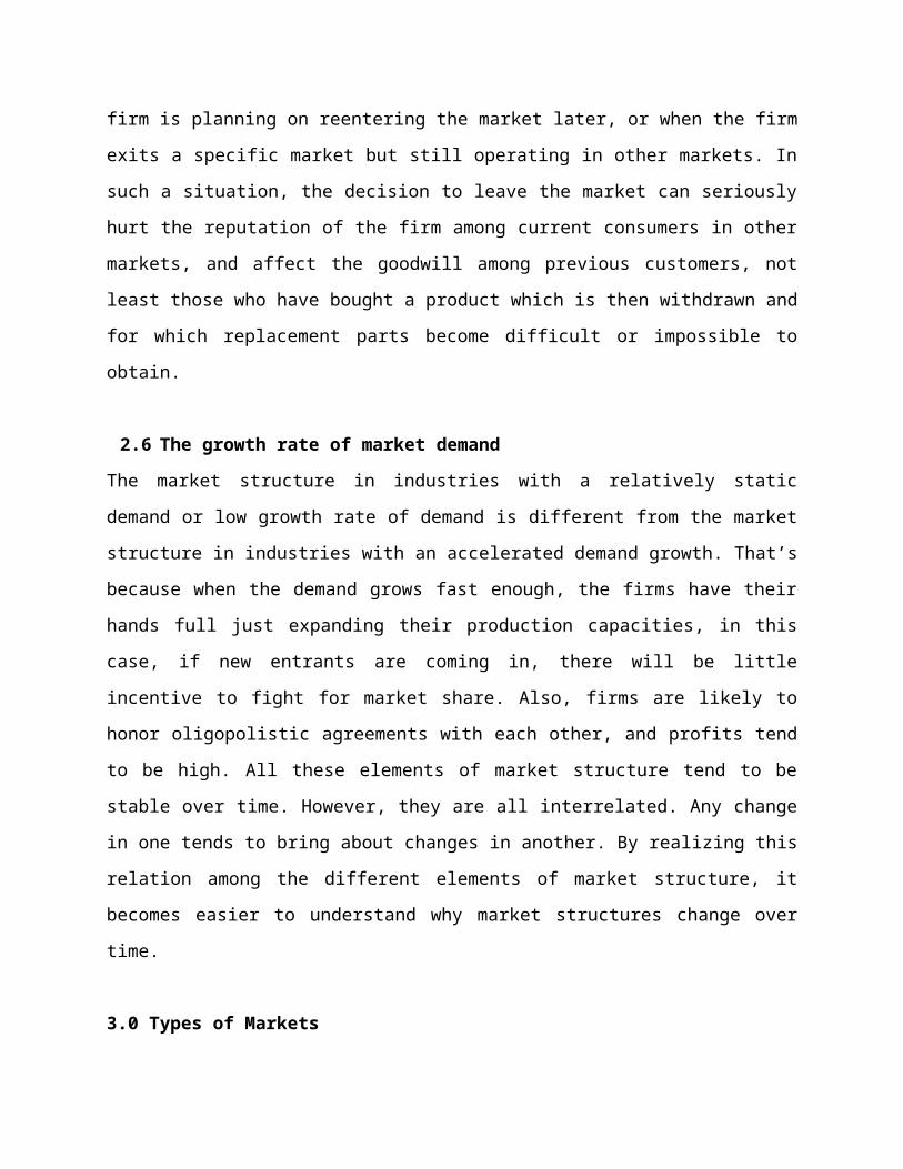
2.6 The growth rate of market demand

The market structure in industries with a relatively static demand or low growth rate of demand

is different from the market structure in industries with an accelerated demand growth. That’s

because when the demand grows fast enough, the firms have their hands full just expanding

their production capacities, in this case, if new entrants are coming in, there will be little

incentive to fight for market share. Also, firms are likely to honor oligopolistic agreements with

each other, and profits tend to be high. All these elements of market structure tend to be stable

over time. However, they are all interrelated. Any change in one tends to bring about changes

in another. By realizing this relation among the different elements of market structure, it

becomes easier to understand why market structures change over time.

3.0 Types of Markets

Using structure we can classify markets as follows

a) Perfect/ Pure Competitive Market

b) Imperfect competitive market

3.1 Perfect/ Pure Competitive Market

This is a type of marketing structure where you have a large number of buyers and sellers and

the contribution of one buyer or seller cannot affect the price.

3.1.1 Assumptions for Pure Competitive MarketI. Large number of buyers and sellers so that individuals cannot influence on price

II. Product homogeneity

III. Free entry and exit

IV. Profit maximization

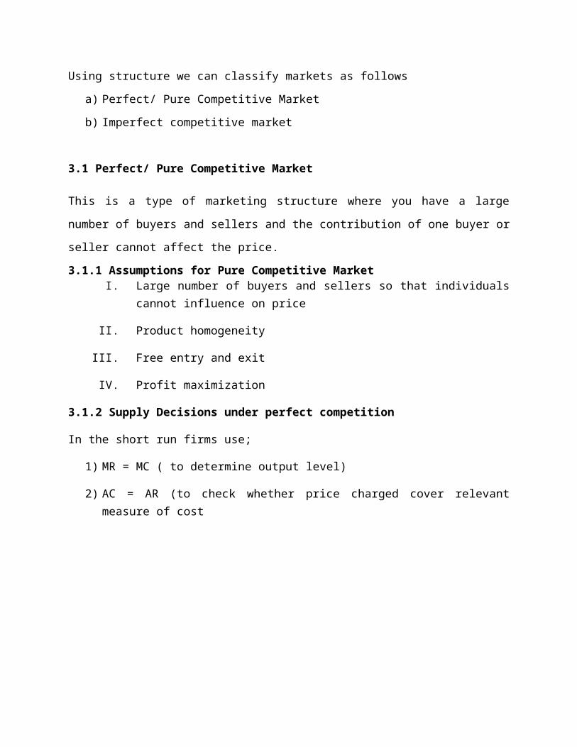
3.1.2 Supply Decisions under perfect competition

In the short run firms use;

1) MR = MC ( to determine output level)

2) AC = AR (to check whether price charged cover relevant measure of cost

MC

AR = MR = P

P

Q

AC

Supply Decisions under perfect competition

Q

AVC (short run)

SAC (short run)

A

C

D

P1

P2

P3

P4

MR

MR

MR

Q1 Q2 Q3 Q4

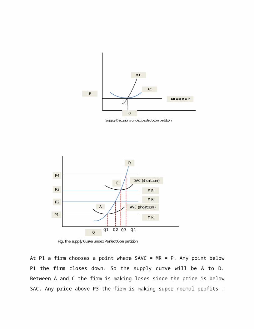
Fig. The supply Curve under Perfect Competition

At P1 a firm chooses a point where SAVC = MR = P. Any point below P1 the firm closes down. So

the supply curve will be A to D. Between A and C the firm is making loses since the price is

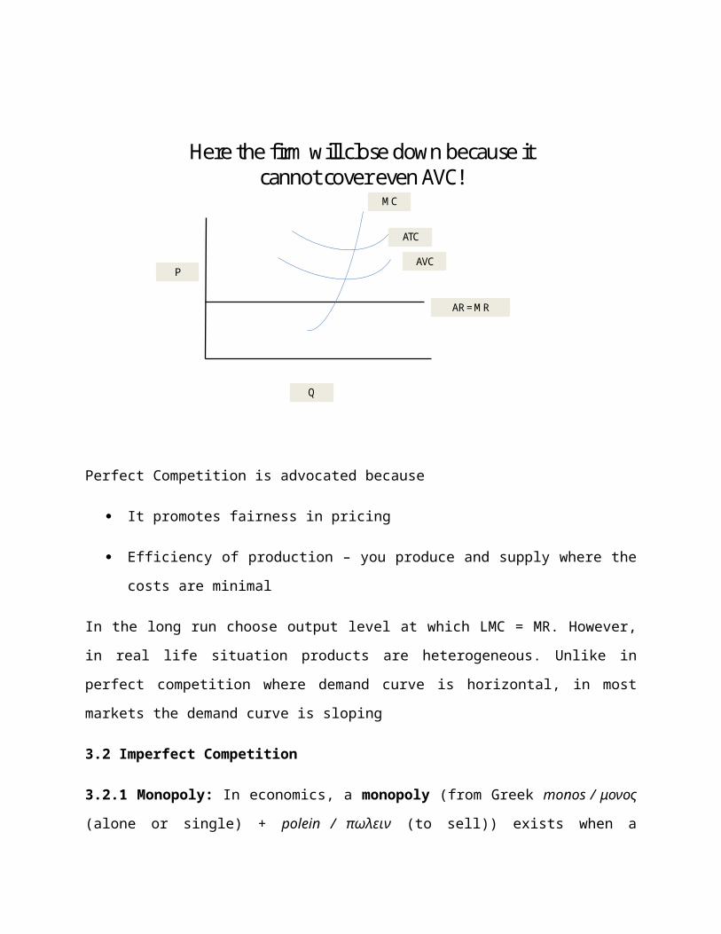
below SAC. Any price above P3 the firm is making super normal profits .

Here the firm will close down because it cannot cover even AVC!

MC

ATC

AVC

AR = MR

P

Q

Perfect Competition is advocated because

It promotes fairness in pricing

Efficiency of production – you produce and supply where the costs are minimal

In the long run choose output level at which LMC = MR. However, in real life situation products

are heterogeneous. Unlike in perfect competition where demand curve is horizontal, in most

markets the demand curve is sloping

3.2 Imperfect Competition

3.2.1 Monopoly: In economics, a monopoly (from Greek monos / μονος (alone or single) +

polein / πωλειν (to sell)) exists when a specific individual or an enterprise has sufficient control

over a particular product or service to determine significantly the terms on which other

individuals shall have access to it. Monopolies can form naturally or through vertical or

horizontal mergers. A monopoly is said to be coercive when the monopoly firm actively

prohibits competitors from entering the field or punishes competitors who do.

3.2.2 Characteristics of a monopolist market

Single seller: In a monopoly there is one seller of the monopolized good who produces

all the output. Therefore, the whole market is being served by a single firm, and for

practical purposes, the firm is the same as the industry.

Market power: Market power is the ability to affect the terms and conditions of

exchange so that the price of the product is set by the firm (price is not imposed by the

market as in perfect competition). Although a monopoly's market power is high it is still

limited by the demand side of the market. A monopoly faces a negatively sloped

demand curve not a perfectly inelastic

3.2.3 Sources of monopoly power

Monopolies derive their market power from barriers to entry - circumstances that prevent or

greatly impede a potential competitor's entry into the market or ability to compete in the

market. There are three major types of barriers to entry; economic, legal and deliberate.

Economic barriers: Economic barriers include economies of scale, capital requirements,

cost advantages and technological superiority.

Economies of scale: Monopolies are characterized by declining costs over a relatively

large range of production. Declining costs coupled with large start up costs give

monopolies an advantage over would be competitors. Monopolies are often in a

position to cut prices below a new entrant's operating costs and drive them out of the

industry.

Capital requirements: Production processes that require large investments of capital, or

large research and development costs or substantial sunk costs limit the number of

firms in an industry. Large fixed costs also make it difficult for a small firm to enter an

industry and expand.

o Technological superiority: A monopoly may be better able to acquire, integrate

and use the best possible technology in producing its goods while entrants do

not have the size or fiscal muscle to use the best available technology. In plain

English one large firm can sometimes produce goods cheaper than several small

firms.

o No substitute goods: A monopoly sells a good for which there is no close

substitutes. The absence of substitutes makes the demand for the good

relatively inelastic enabling monopolies to extract positive profits.

o Control of Natural Resources: A prime source of monopoly power is the control

of resources that are critical to the production of a final good.

Legal barriers: Legal rights can provide opportunity to monopolise the market in a good.

Intellectual property rights, including patents and copyrights, give a monopolist

exclusive control over the production and selling of certain goods. Property rights may

give a firm the exclusive control over the materials necessary to produce a good.

Deliberate Actions: A firm wanting to monopolise a market may engage in various types

of deliberate action to exclude competitors or eliminate competition. Such actions

include collusion, lobbying governmental authorities, and force.

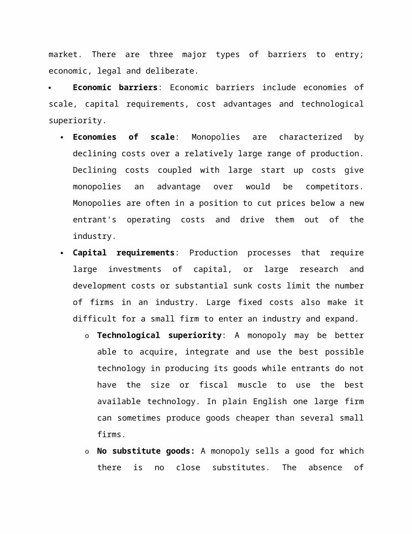
Demand curve is downward sloping (Since no market is perfect). This reflects changes in price

as you vary the output. A monopolist will have supernormal profit by charging high prices.

P1

P2

AR = D

Q1 Q2

By increasing price, you lose some customers and demand decreases

Firms will equate MR = MC to maximize profit

In this case AR is > AC which implies firms under monopoly get supernormal profit

MC

DemandMR

AC

Po

P1 B

A

Q

O

P1, B, A,Po represent supernormal profit while O, Po, A, E represent TC

E

Price Po would have been the price but a monopolist would charge P1 since he is able control

the supply. P1, B, A,Po represent supernormal profit while O, Po, A, E represent Total Cost.

While in perfect competition firms are price takers, in monopoly firms are price setter ie. having

decided the level of output they would then decide on how much to charge. Absence of a

supply curve is an aspect of monopoly because a monopolist output has effect on MR and MC.

So a monopolist doesn’t have a supply curve. Simultaneously he/she decides on the supply as

well as the price.

MC

AC

DMR

Q

P

3.3 Criticisms of monopoly

Inefficiency of society’s resource use

Unfair pricing to consumers

Fig 1 showing how a Monopolist sets the price

Surpluses and deadweight loss created by monopoly price setting. According to the standard

model in which a monopolist sets a single price for all consumers, the monopolist will sell a

lower quantity of goods at a higher price than would firms under perfect competition. Because

the monopolist ultimately forgoes transactions with consumers who value the product or

service more than its cost, monopoly pricing creates a deadweight loss referring to potential

gains that went neither to the monopolist or to consumers. Given the presence of this

deadweight loss, the combined surplus (or wealth) for the monopolist and consumers is

necessarily less than the total surplus obtained by consumers under perfect competition.

Where efficiency is defined by the total gains from trade, the monopoly setting is less efficient

than perfect competition.

3.4 Interventions in a Monopoly market

When monopolies are not broken through the open market, sometimes a government will step

in, either to regulate the monopoly, turn it into a publicly owned monopoly environment, or

forcibly break it up. You can break up a monopoly by introduction of new firms. This will shift

the demand to the left.

Public utilities, often being naturally efficient with only one operator and therefore less

susceptible to efficient breakup, are often strongly regulated or publicly owned.

The government can set price controls which will force firm to sell more if they want to

maximize profits. This will protect the consumers. Government can break up monopolies by

encouraging competition. Encourage firms to produce at a point where AC is minimum. It may

also nationalize the firms.

The govt. can also introduce tax if there are supernormal profits. It can either tax the profit or

tax the output. Introducing a tax will increase firm’s Average Costs thereby reducing

supernormal profits.

4.0 Oligopoly Market

An oligopoly ((from Ancient Greek ὀλίγοι (oligoi) "few" + πωλειν (polein) "to sell") is a market

form in which a market or industry is dominated by a small number of sellers (oligopolists). The

word is derived, by analogy with "monopoly", from the Greek oligoi 'few' and poleein 'to sell'.

Because there are few sellers, each oligopolist is likely to be aware of the actions of the others.

The decisions of one firm influence, and are influenced by, the decisions of other firms.

Strategic planning by oligopolists needs to take into account the likely responses of the other

market participants. This causes oligopolistic markets and industries to be a high risk for

collusion. This is also referred to as competition among the few. This is the most prevalent

market structure. The industry is dominated by small number of large firms and each firm has a

large market share - output of each firm is large enough to affect the market. Their products are

highly differentiated in a number of ways

• Quality designs

• Heavy adverts

• Packaging and labelling

There is little actual collusion among firms. However to determine price the firm has to

consider the effect of the price on other firms. One firm cannot ignore the existence of other

firms.

4.1 Assumptions under oligopoly

• Few firms in the market

• Product differentiation- oligopolies might also create excessive levels of differentiation

in order to stifle competition.

• Firms have identical cost functions

• Price is a strategic issue – if one firm raise the price the other will not in order to benefit

from the other firm

4.2 Behaviour of Oligopolistic firms

Oligopolistic competition can give rise to a wide range of different outcomes. In some

situations, the firms may employ restrictive trade practices (collusion, market sharing etc.) to

raise prices and restrict production in much the same way as a monopoly. Where there is a

formal agreement for such collusion, this is known as a cartel. A primary example of such a

cartel is OPEC which has a profound influence on the international price of oil.

Firms often collude in an attempt to stabilise unstable markets, so as to reduce the risks

inherent in these markets for investment and product development. There are legal restrictions

on such collusion in most countries. There does not have to be a formal agreement for collusion

to take place (although for the act to be illegal there must be actual communication between

companies) - for example, in some industries, there may be an acknowledged market leader

which informally sets prices to which other producers respond, known as price leadership.

In other situations, competition between sellers in an oligopoly can be fierce, with relatively low

prices and high production. This could lead to an efficient outcome approaching perfect

competition. The competition in an oligopoly can be greater than when there are more firms in

an industry.

4.3 Demand Curve for Oligopoly Model

The demand curve is kinked downwards. This shows;

• No rivalry price reaction for price increases

• For price reduction you expect rivals to exactly match the price reduction to maintain

market share

"Kinked" demand curves have in common with traditional demand curves that they are

downward-sloping. They are distinguished by a hypothesized convex bend with a discontinuity

at the bend - the "kink." Therefore, the first derivative at that point is undefined and leads to a

jump discontinuity in the marginal revenue curve.

MC

AC

DMR

Q

p

MR

D1

D’

Fig. Kinked demand curve under Oligopoly

According to this model, each firm faces a demand curve kinked at the existing price. The

conjectural assumptions of the model are (1) if a firm raises its price above the existing price

competitor will not follow and the acting firm will lose market share (2) if a firm lowers price

below the existing price then competitors will follow to preserve their market share and the

acting firm's output will increase only slightly.

If the assumptions hold then:

The firm's marginal revenue curve is discontinuous, has a gap, at the kink For prices above the

prevailing price the curve is relatively elastic For prices below the point the curve is relatively

inelastic . The gap in the marginal revenue curve means that marginal costs can fluctuate

without changing equilibrium price and quantity. Thus prices tend to be rigid.

The motivation behind this kink is the idea that in an oligopolistic or monopolistically

competitive market, firms will not raise their prices because even a small price increase will lose

many customers. However, even a large price decrease will gain only a few customers because

such an action will begin a price war with other firms. The curve is therefore more price-elastic

for price increases and less so for price decreases.

If you produce <Q it means MR< MC – Loss. A firm’s current price and output levels are P and

Q. Above P, a relatively inelastic ceteris paribus demand curve exists D1D’. Below P the

demand curve is relatively elastic mutatis mutandis D’D

Price rigidity despite changing demand levels

Price rigidity despite changing demand levels

D1

D

D1

D

MC

A1

MR

C

B

Q1

PriceB1

MR1

Q

P

Suppose original demand curve is D1D1. If there is pressure to increase demand to DD,

Normally you would increase price but here you increase output to take into account the

increased demand without increasing price. Demand could fluctuate between Q to Q1 at price

P without a firm wishing to change its price. Profits are lower when demand is lower but are

maximized at price P as long as demand shift is not high so as to cause MC curve to change

greatly

Price rigidity despite changes in cost

D1

D1 MC1

MR

C

B

Q1

Price

P

MC2

You could produce Q1 at MC1. If all of sudden the cost changes to MC2, the change should

not affect price if the firm is still able to make supernormal profit. A firm is unwilling to

change price as long as MR > MC.

45°

60

60

Price preferred by Firm 1

Price preferred by Firm 1

For firms that depend on activities of other firms in its pricing policy, equilibrium is reached

when the 2 firms charge equal prices

4.4 Dominant firm model

In some markets there is a single firm that controls a dominant share of the market and a group

of smaller firms. The dominant firm sets prices which are simply taken by the smaller firms in

determining their profit maximizing levels of production. This type market is practically a

monopoly and an attached perfectly competitive market in which price is set by the dominant

firm rather than the market. equating price to marginal costs.

The demand curve for the dominant firm is determined by subtracting the supply curves of all

the small firms from the industry demand curve. After estimating its net demand curve (market

demand less the supply curve of the small firms) the dominant firm maximizes profits by

following the normal p-max rule of producing where marginal revenue equals marginal costs.

The small firms maximize profits by acting as PC firms

4.5 Cournot-Nash model

The Cournot-Nash model is the simplest oligopoly model. The models assumes that there are

two “equally positioned firms”; the firms compete on the basis of quantity rather than price

and each firms makes an “output decision assuming that the other firm’s behavior is fixed.” The

market demand curve is assumed to be linear and marginal costs are constant.

To find the Cournot-Nash equilibrium one determines how each firm reacts to a change in the

output of the other firm. The path to equilibrium is a series of actions and reactions.The pattern

continues until a point is reached where neither firm desires “to change what it is doing , given

how it believes the other firm will react to any change.

The equilibrium is the intersection of the two firm’s reaction functions. The reaction function

shows how one firm reacts to the quantity choice of the other firm. For example, assume that

the firm 1’s demand function is P = (60 - Q2) - Q1 where Q2 is the quantity produced by the other

firm and Q1 is the amount produced by firm 1. Assume that marginal cost is 12. Firm 1 wants to

know its maximizing quantity and price.

Firm 1 begins the process by following the profit maximization rule of equating marginal

revenue to marginal costs. Firm 1’s total revenue function is PQ = Q1(60 - Q2 - Q1) = 60Q1- Q1Q2 -

Q12. The marginal revenue function is MR = 60 - Q2 - 2Q.

MR = MC

60 - Q2 - 2Q = 12

2Q1 = Q2 - 48

Q1 = 0.5Q2 - 24 [1.1]

Q2 = 2Q1 + 48 [1.2]

Equation 1.1 is the reaction function for firm 1. Equation 1.2 is the reaction function for firm 2.

To determine the Cournot-Nash equilibrium you can solve the equations simultaneously. The

equilibrium quantities can also be determined graphically. The equilibrium solution would be at

the intersection of the two reaction functions. Note that if you graph the functions the axes

represent quantities. The reaction functions are not necessarily symmetric. The firm’s may face

differing cost functions in which case the reaction functions would not be identical nor would

the equilibrium quantities.

Under oligopoly there is price rigidity despite changes in demand curve and cost function.

4.6 Barriers to entry

• Price cutting• Merger• Integration

Criticism of the model is that it assumes firms have more or less identical production costs.

A new firm may develop a technology that reduces costs.

5.0 Market Conduct

This implies what firms do to compete with each other. It includes pricing, advertising, research

and development investment, decisions on product dimensions, merger and acquisition, etc.

Conduct also can include collusion both explicit or tacit. In examining conduct we look at how

the market structure affect pricing, output and other decisions of businesses within the market.

Some questions that are asked include;

• Are there dominant firms?

• Is there evidence of anti-competitive behaviour?

– Collusive pricing agreements

– Predatory pricing?

– Vertical restraint?

• How important is non-price competition in the market?

• Is there interdependence between firms?

• Do businesses behave strategically to retain profits by deterring the entry of new

competitors in the long run?

Be aware that the market structure will affect the behaviour of firm

6.0 market Performance

The performance of an industry or firm is measured by profitability. Profit is the difference

between revenue and cost, and revenue is determined by price. Thus performance can be

influenced through changing costs or prices. Profitability can also be affected by a firm’s agility

(i.e. ability to adjust to things like changes in market demand). Research and development, and

availability of capitol and resources are factors that greatly influence whether or not a firm is

agile. The ability to measure performance between industries is important in understanding the

SCP relationships. For example, if an industry is dominated by one firm or cartel does not see

higher costs than a competitive industry yet has monopoly prices, then that non-competitive

industry will see higher profits, whereas if costs increase, then profitability levels will be

relatively similar. This comparison is the driving force behind anti-trust legislation. SCPP

predicts that performance increases with concentration of the industry. This is in contrast with

the efficiency hypothesis that states that a firms performance is based on how well and

efficiently it produces its product for the consumer.

It is believed that the number of firms on the market will influence the individual behavior of

the firms which will affect the performance of the market. However it has also been argued that

conduct of the firms may affect the structure of the market. For example, if the firms are hostile

to each other, other firms will fold up leaving few firms on the market or they may merge with

the big firms.

5.0 Learning Activities

Assignments - explaining with the aid of diagrams how different market system would react if

there are changes in production or prices.

6.0 Summary of Topic

In this topic you have learnt that there are different types of market systems. Pure Competitive

market is the most efficient one although most markets are oligopoly. You have also learnt that

monopolies can occur naturally, or by behaviour of a firm as well as due to government

regulations. Monopolies can be broken by introduction of new firms as well as introduction of

regulations. It was noted that market structure influences market conduct which affects the

performance of a market. It has also been argued that the converse may be true where market

performance will affect the conduct of the firms thereby affecting the structure.

Market structure

Conduct of Firms Performance

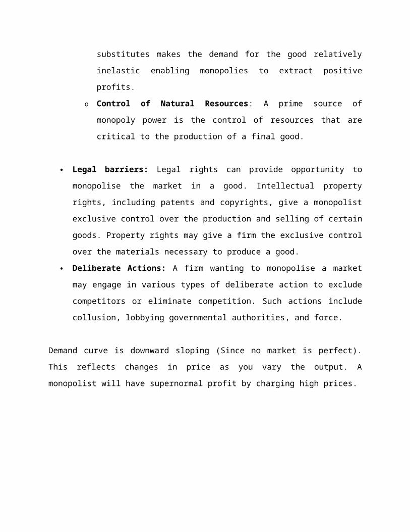
Further Reading Materials

Cabral, Luís M. B. (2000). Introduction to Industrial Organization. MIT Press

Ayers & Collinge, Microeconomics (Pearson 2003)

Useful Links

www.egwald.ca/economics/index

www.regulationbodyofknowledge.org/chapter2/narrative/1/

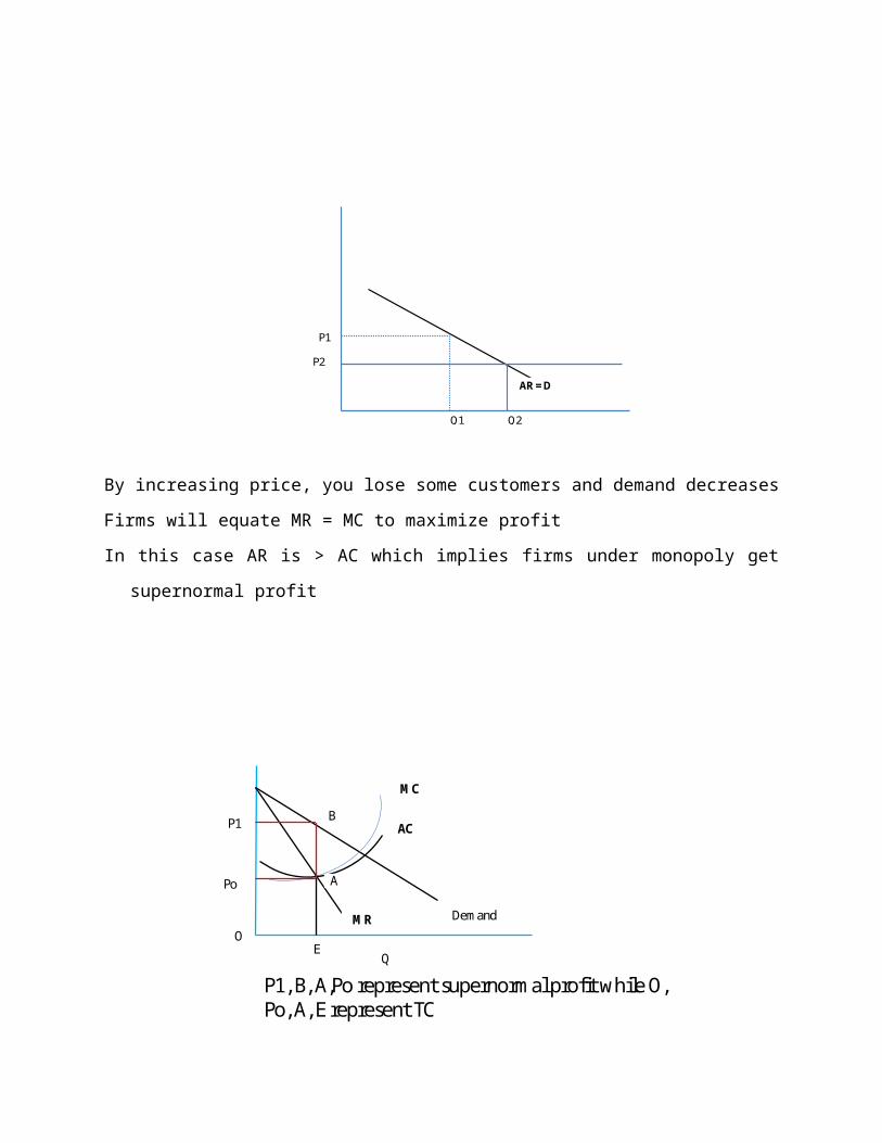
Topic 5: Time Value of Money

Learning Outcomes

Upon completion of this lesson you will be able to;

Calculate Present Value of a future sum and future value of a presnt sum.

Apply knowledge of time-value of money in investment decisions.

Key Terms: Present Value, Future Value, Discounting, Compounding

1.0 Introduction to Time Value of Money

Time value of money is based upon the economic fact that $1 today is worth more than a

promise of $1 at some future date because of its current earnings potential. Time value of

money helps a producer to decide whether to receive payment now or wait until a future date.

Time value of money can be viewed either within the context of the future value of present

sum or stream of payments or the present value of a future sum or stream of income flows.

Future Value of Money

This is defined as ending value n periods from now of either an investment made today or a

stream of investment made between now and year n. The process of computing the future

value of money is called compounding. For example, we may want to know the future value of

$1000 invested now at a specific rate of interest will be one period (P1), two periods (P2) or n

periods (Pn) from now

Future Value (Compounding)

P1 P2 P3 Pn

NOW N periods from Now

Future Value of a present sum

In calculating the future value (FV) of a present sum the following formula is used;

.

Where PV = Present value

(1+r)n = Interest factor

Letting Po represent the present value of an investment (how much you plan to invest now) and

we want to know what its future value will be n periods from now (Pn). We must compound

the present value Po over n periods at the periodic interest r

Example

The future value of $1,000 invested at an annual rate of interest of 5% after 5 years would be

equal to;

P5 = $1,000 (1+0.05)5

= $1,000 (1.276)

= $1,276

Looking at the Future Value of $1 Tables shows that FIF5,5 = 1.276 which also gives P5 = $1,276

Applicability

Suppose a farmer is considering retiring from farming in 10 years time and would like to know

what the market value of his land will be at that time. Suppose land value have been increasing

at the rate of approximately 6% annually and if the land is currently worth $1,000 an acre, its

value in 10 years from now would be;

P10 = $1,000 (1+0.06)10

= $1,000 (1.791)

= $1,791

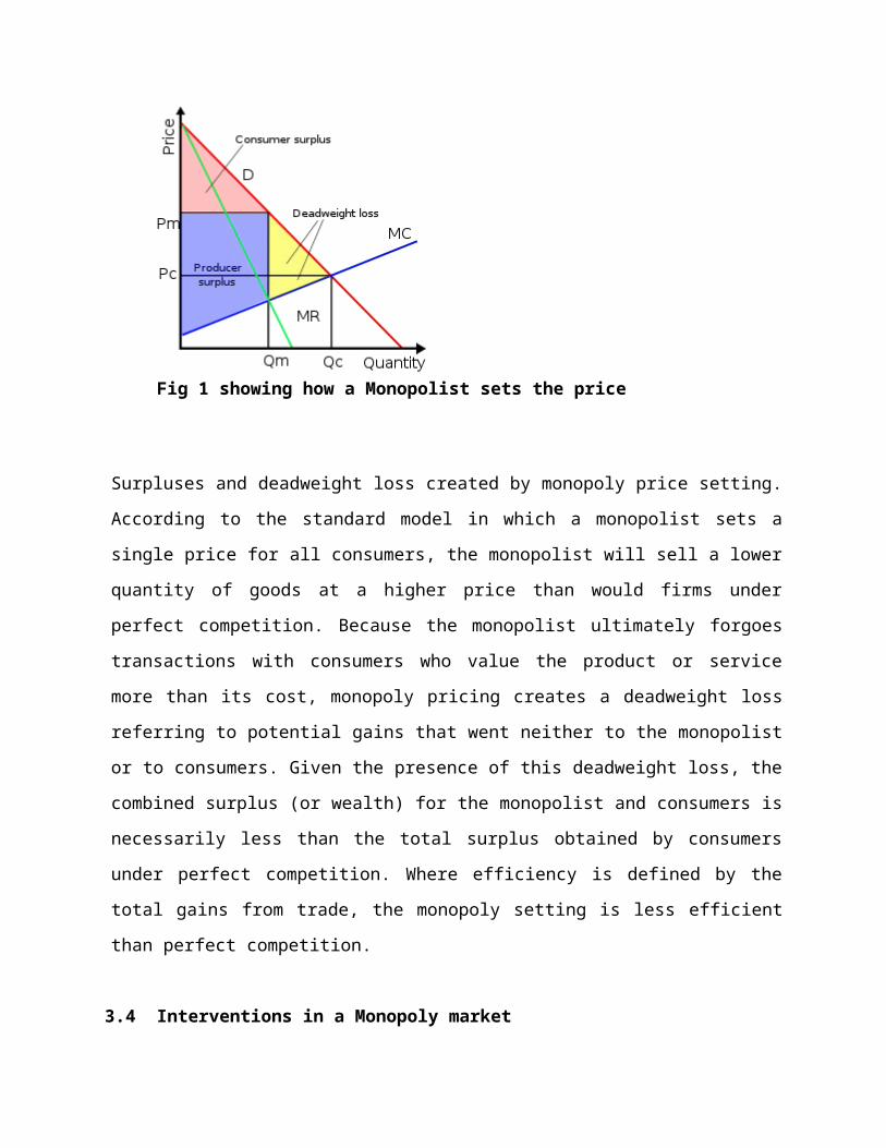
Future Value of a Stream of Investments

In the previous sub-topic we looked at future value of a present sum. Frequent use of future

value or compounding is in the analysis of annuities.

Suppose there are streams of payments over the years, how do we calculate the future value

of these annuities? There are two types of annuities namely regular annuities (series of

payments of equal value at the end of each year over a specified period of time) and differed

annuities (different amount of payments over time). To calculate the future value of these two

different formulas are used.

For example, assume that you are to receive an annuity paying $1,000 at the end of each year

for the next 5 years. How much would you have received at the end of 5 th year if the rate of

interest is 5%?

One approach is to compute the future value of a present sum for each period and then add

them together

Pn = A1(1+r)n-1 + A2(1+r)n-2 +…+ An(1+r)n-n

where A1 represents the annuity payment reinvested in year 1 and so on

Another approach is to multiply the annuity payment by the Future Value Interest Factor (FIF)

from the Future value equal payment tables for the number of years and rate of interest in

question.

= A1(FIFr,n-1) + A2(FIFr,n-2) +…+ An

Using the first approach, the future value is calculated as;

P5 = $1,000(1+0.05)4 + $1,000(1+0.05)3 +$1,000(1+0.05)2 + $1,000(1+0.05)1 +

$1,000(1+0.05)0

= $1,000(1.216) + 1,000(1.158) + 1,000(1.103) + 1,000(1.050) + 1,000

= $5,526

Equal payment-future value interest factors

For equal annuity payments, we can find the EFIFr,n which would be multiplied by the annuity to

find the future value.

Pn = Ae(EFIF r,n)

Where Ae represent the equal periodic payments. In the preceding example the value of

annuity was $1,000, r = 0.05, n = 5 years

P5 = $1,000(5.526) = $5,526

Other applications

Suppose that you are interested in knowing the amount of funds you must invest out of your

current income at the end of every year in a savings account paying 5% interest in order to

accumulate $5,526 at the end of 5 years.

Pn = Ae(EFIF r,n)

Ae = Pn/ (EFIF r,n)

= $5,526/5.526

= $1,000

Relationship between FIFr,n and EFIFr,n

The EFIFr,n is related to FIFr,n by the following formula;

EFIFr,n = FIFr,n – 1.0

r

Present value

Refers to the value of money today of a payment received n periods from now or a series of

income flows received over n periods. Knowledge in present value helps to decide whether one

should accept a promise of future payment or receive payment now. To help in deciding

between these alternatives, a producer can compute the present value of the future payment.

Discounting

The computational process used to find the present value of a future payment or flow of

income is referred to as discounting.

Present value of a future sum

Let Pn represent future value of a payment (what you will receive in cash) n periods from now

and we want to know what's its present value (Po) now.

To find the value we must discount Pn back n periods by the rate of return we could have

received from out next best opportunity (usually we use the bank interest rate). The following

formula is used

Years

NOW 1 2 n

Discounting process

Po = Pn

(1+r)n

Or

Po = Pn (PIFr,n)

where PIFr,n is the present value interest factor or 1/(1+r)n (PIF is found in the Tables)

Example

What is the present value of $1,276 promised 5 years from now if the rate of interest is 5%.

Po = $1,276

(1+0.05)5

= $1,276(0.784)

= $1,000

Or

= $1,276(PIF0.05,5)

= $1,276(0.784)

= $1,000

Present value of a stream of Income

Suppose that you wanted to know what the value of a stream of income consisting of equal

annual receipts of $1,000 over 5-year period. If they were invested as they were received the

rate of interest being 5%, the present value would be;

P0 = Y1 + Y2 +…+ Yn

(1+r)1 (1+r)2 (1+r)n

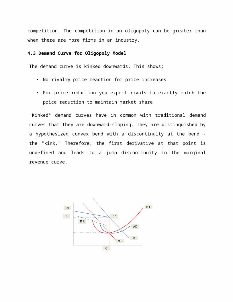
= Y1(PIFr,n) + Y2(PIFr,n) +…+ Yn(PIFr,n)

= 1000(PIF0.05,1) + 1000(PIF0.05,2) + 1000(PIF0.05,3) + 1000(PIF0.05,4) + 1000(PIF0.05,5)

= 1000(0.952) + 1000(0.907) + 1000(0.864) + 1000(0.823) + 1000(0.784)

= $4,329

Thus given the opportunity of earning 5% interest on your money, you should never be willing

to invest more than $4,329 to secure an asset paying $1,000 annually over a period of 5 years.

Equal Periodic Income Flows

In case of equal periodic income cashflow and a constant discount rate, we can simplify the

computational procedure by using tables to get Equal payment present value interest factor

(EPIFr,n)

P0 = Ye(EPIFr,n)

= $1,000(4.329)

= $4,329

Other Applications

To determine the present value of a productive asset having an infinite span like land, we can

reduce the equation

P0 = Ye(EPIFr,n) to simple capitalization formula

P0 = Ye

r

Example: If an acre of land is expected to provide an additional net revenue of $500 to your

business and the discount rate is 5%, The equation above suggests that its capitalized value is

$10,000. Thus you could justify on economic grounds to buy an acre of land at more than

$10,000 per acre unless Ye increases or r declines

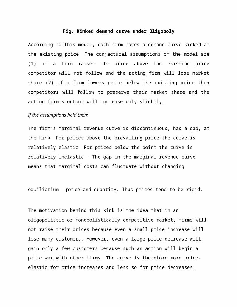
Relationship between FIF and PIF

EPIFr,n = 1 – PIFr,n

r

PIFr,n = 1/FIFr,n for equal value of r and n

We see that where r = 0.05 and n = 5, we get FIF0.05,5 = 1.275 while PIF0.05,5 = 0.784.

Thus we can see that

1/FIF0.05,5 = PIF0.05,5

1/1.276 = 0.784

We can see a reciprocal relationship between compounding a present sum and discounting a

future sum.

Learning Activities

Tutorials, Assignments and Quizzes

Summary of Topic

In this topic you have learnt that the value of $1 today is not the same as $1 future. You have

also learnt that present value and future value techniques help in deciding whether to accept

payment now or wait for the future. With examples, you have seen how the two concepts are

used in fisheries and aquaculture planning.

Further Reading Materials

Jolly, C.M., and Clonts, H. A. (1993). Economics of Aquaculture. Food Products Press, an

Imprint of the Hearth Press, Inc.,

Crosson, S.V., and Needles, B.E.(2008). Managerial Accounting (8th Ed). Boston:

Houghton Mifflin Company.

Useful Links

http://en.wikipedia.org/wiki/Time_value_of_money

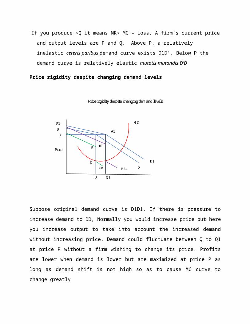
Topic 6: Cost Benefit Theory

Learning Outcomes

Upon completion of this lesson you will be able to;

Determine the economic viability of an investment how to incorporate elements of cost-benefit analysis into policy work; Decide when CBA is a good tool to use and when it isn’t.

Key Terms: Benefit-Cost ratio, Net Present Value

1.0 Introduction to Cost benefit theory

Cost–benefit analysis is often to evaluate the desirability of a given intervention. It is an analysis of the cost effectiveness of different alternatives in order to see whether the benefits outweigh the costs. The aim is to gauge the efficiency of the intervention relative to the status quo. The costs and benefits of the impacts of an intervention are evaluated in terms of the public's willingness to pay for them (benefits) or willingness to pay to avoid them (costs). Inputs are typically measured in terms of opportunity costs - the value in their best alternative use. The guiding principle is to list all parties affected by an intervention and place a monetary value of the effect it has on their welfare as it would be valued by them.

The process involves monetary value of initial and ongoing expenses vs. expected return. Constructing plausible measures of the costs and benefits of specific actions is often very difficult. In practice, analysts try to estimate costs and benefits either by using survey methods or by drawing inferences from market behavior. For example, a product manager may compare manufacturing and marketing expenses with projected sales for a proposed product and decide to produce it only if he expects the revenues to eventually recoup the costs. Cost–benefit analysis attempts to put all relevant costs and benefits on a common temporal footing. A discount rate is chosen, which is then used to compute all relevant future costs and benefits in present-value terms. Most commonly, the discount rate used for present-value calculations is an interest rate taken from financial markets (R.H. Frank 2000). This can be very controversial; for example, a high discount rate implies a very low value on the welfare of future generations, which may have a huge impact on the desirability of interventions to help the environment. Empirical studies suggest that in reality, people's discount rates do decline over time. Because cost–benefit analysis aims to measure the public's true willingness to pay, this feature is typically built into studies.

During cost–benefit analysis, monetary values may also be assigned to less tangible effects such as the various risks that could contribute to partial or total project failure, such as loss of

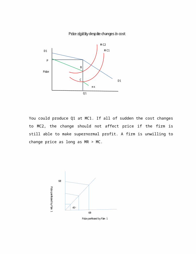
reputation, market penetration, or long-term enterprise strategy alignments. This is especially true when governments use the technique, for instance to decide whether to introduce business regulation, build a new road, or offer a new drug through the state healthcare system. In this case, a value must be put on human life or the environment, often causing great controversy. For example, the cost–benefit principle says that we should install a guardrail on a dangerous stretch of mountain road if the dollar cost of doing so is less than the implicit dollar value of the injuries, deaths, and property damage thus prevented (R.H. Frank 2000).

Cost–benefit calculations typically involve using time value of money formulas. This is usually done by converting the future expected streams of costs and benefits into a present value amount.

Set of key cost–benefit indicators, including the following:

NPV (net present value) PVB (present value of benefits)

PVC (present value of costs)

BCR (benefit cost ratio = PVB / PVC)

Net benefit (= PVB - PVC)

NPV/k (where k is the level of funds available)

2.0 Steps in calculating Benefit-cost ratio

The calculation of B-C ratio involves the following;

Quantifying all the benefits and costs involved in the proposal and its alternatives (all benefits and costs are assigned an monetary value)

Discount all the benefits and costs to obtain figures representing a value of all benefits and costs in the present time

Divide the discounted benefits by discounted costs B-C Ratio = ∑ Bt / Ot + K

(1+r)t (1+r)t

Where Bt = discounted benefits Ot = discounted costs

1/(1+r)t = discounting factors r = Interest factor

t = no. of years

K = investment capital

2.1 Example of Benefit-Cost Analysis assuming a discounting rate of 10%

Year Equipment

wages materials Benefits

undiscounted

Discounted

Undiscounted

discounted

undiscounted

Discounted

0 US1,000 100

1 150 90.91 200 181.82 500 454.55

2 250 123.96 250 206.60 700 578.48

3 250 187.52 350 262.95 1000 751.30

4 250 170.75 350 239.05 1000 683.00

5 250 155.23 350 217.31 1000 620.90

Totals

1,000 728.67 1,107.73 3088.23

Present value of Benefits = US$3,088.23

Present value of costs = 1,000+728.67+ 1107.73

= US$2,836.40

Benefit-cost Ratio = 3088.23/2836.40

= 1.09

According to the principle of Benefit cost analysis you choose a project whose ratio is greater than 1 (more benefits than costs). B-C ratio = 1 means break-even.

2.3 What if you have two projects with B-C ratio greater than 1?

Rank projects in increasing cost of investment and operation (start with smallest to largest). Compute incremental B-C ratio.

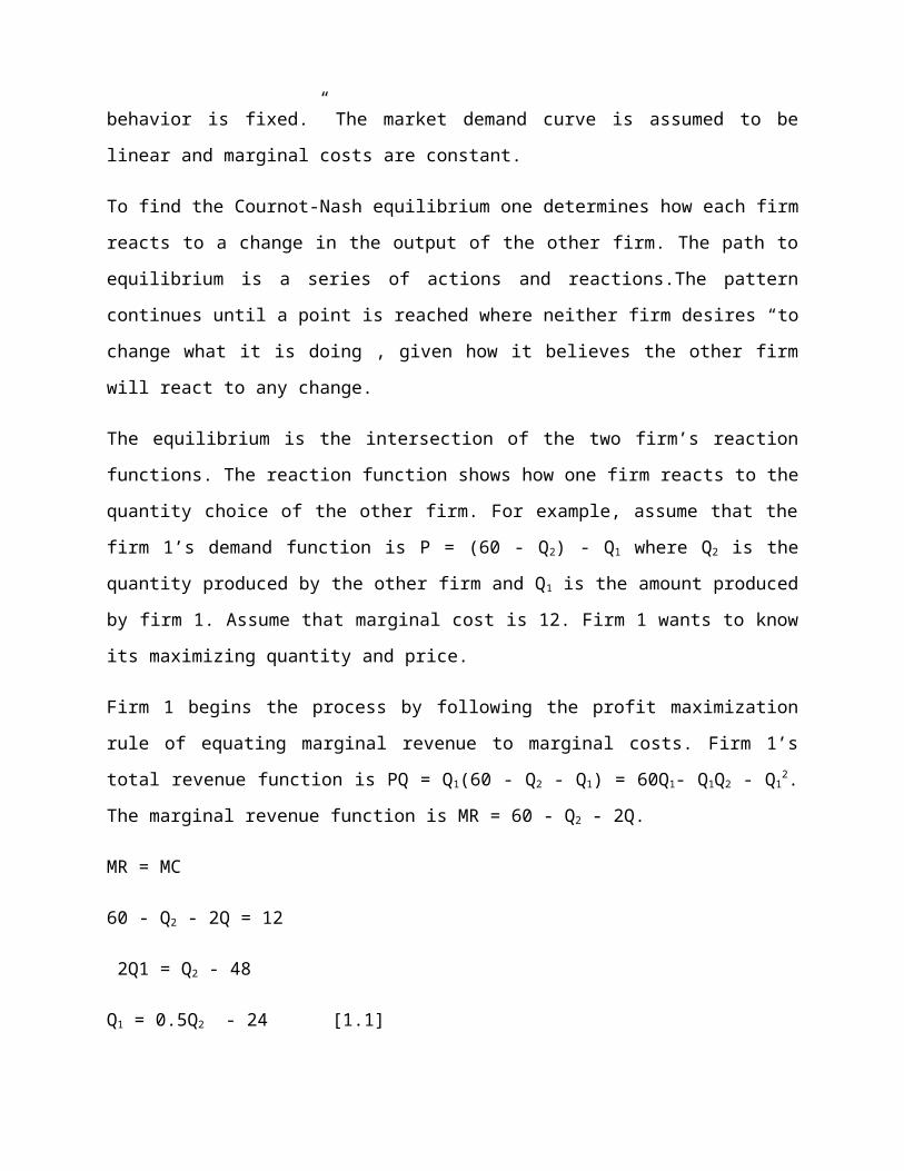
Project Benefit Cost B-C ratio Incremental

Benefit Cost

B-C ratio

A 1000 500 2.00 - - -

B 1450 700 2.07 450 200 2.25

C 1900 1000 1.90 450 300 1.5

D 2000 1200 1.67 100 200 0.5

3.0 Net Present Value

Net Present value is the present value of net revenue of an investment (including the investment cost)

Where the discounting rate is constant the entire project life, the Net Present Value is

NPo = Y1 + Y2 +…+ Yn - C

(1+r)1 (1+r)2 (1+r)n

= Y1(PIFr,1) + Y2(PIFr,2) +…+ Yn(PIFr,n) - C

Where;

Yi = net cash revenue flows

C = Original investment cost

r = Discounting rate

Project A is already excluded by ranking it first. B-C analysis tend to favour capital intensive investmentD is excluded because it has B-C ratio of less than 1B and C have B-C ration of greater than 1.Choose B because it has the highest B-C ratio

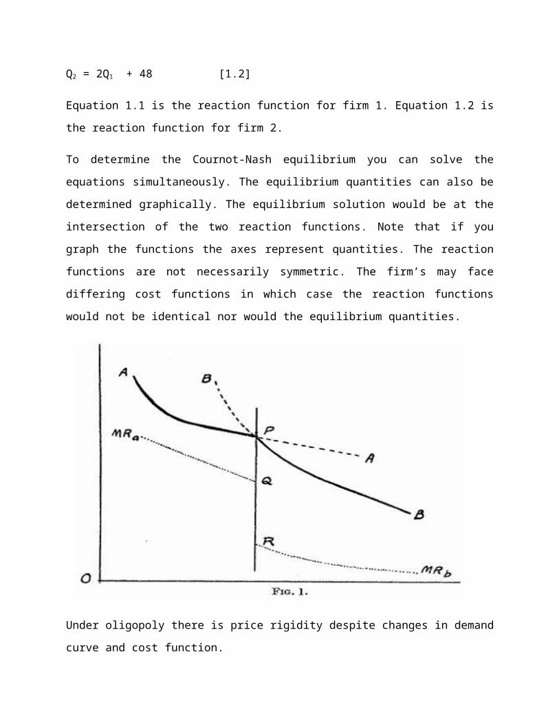
3.1 Decision making rule

Accept a project with NPV > 0

NPV = 0 means you will be indifferent

NPV < 0 reject the project

NPV can be viewed as a profit of making the investment

3.2 Example

Assume you have two projects with initial investment of $10,000, 5% discount rate and 5 years economic life.

Project A Project B

Year

i

Net cash flow

PIF0.05,i Present value of Yi

Net Cash flow

PIF0.05,t Present value of Yi

1 3,000 0.952 2,856 2,000 0.952 1,904

2 3,000 0.907 2,721 3,000 0.907 2,721

3 3,000 0.864 2,592 5,000 0.864 4,320

4 3,000 0.823 2,469 2,000 0.823 1,646

5 3,000 0.784 2,352 1,000 0.784 784

Total

Less initial cost

15,000 12,990

-10,000

13,000 11,375

-10,000

NPV $2990 $1375

3.3 Interpretation

The decision rule is that select a project that has a positive NPV. In the example above both Project A and Project B are economically viable because they both have a positive NPV. However Project A is chosen over Project B because it brings in more profit than Project B

Learning Activities

Tutorials, Assignments and Quizzes

Summary of Topic

In this lesson you can learnt on how to evaluate the economic viability of an investment. You

have learnt the before investing in any project, it is important to conduct an analysis to

determine its financial viability. Benefit-cost ratio and Net Present value are some of the

techniques used in such analysi.

Further Reading Materials

Cost-Benefit Analysis: Concepts and Practice, 3rd edition, by Boardman, Greenburg, Vining, and Weimer. (Prentice Hall, 2006).

A Guide to Benefit-Cost Analysis, 2nd edition, by Gramlich (Waveland Press, reissued in 1998).

Guide to Cost-Benefit Analysis of Investment Projects. Evaluation Unit, DG Regional Policy,

European Commission, 2002.

Tevfik F. Nas, Cost-Benefit Analysis: Theory and Application (Thousand Oaks, Ca.: Sage, 1996)

Useful Links

http://www.bepress.com/jbca/

http://www.urban.org/publications/411047.html

Topic 7: Efficient Market Hypothesis - EMH

Learning Outcomes

Upon completion of this lesson you will be able to;

Understand the operations of financial markets Explain the Efficient Market Hypothesis.

Key Terms: Stock market, Risk

1 Introduction to financial market efficiency

Financial market is a market for the exchange of capital and credit, which consists the money markets and the capital markets. Money market is the market for short-term debt securities, which is a typically safe and highly liquidable investment. While capital market is the market where long-term debt or securities are traded.

Market efficiency refers to a condition, in which current prices reflect all the publicly available information about a security. The basic idea underlying market efficiency is that competition will drive all information into the price quickly.

In the financial market, the maximum price that investors are willing to pay for a financial asset is actually the current value of future cash payments that discounted at a higher rate to compensate us for the uncertainty in the cash flow projections. Therefore what investors are trading actually information as a "commodity" in financial market for the future cash flows and information about the degree of certainty.

Efficient market emerges when new information is quickly incorporated into the price so that price becomes information. In other words the current market price reflects all available information. Under these conditions the current market price in any financial market could be the best-unbiased estimate of the value of the investment.

2.1) The theory of Efficient Market Hypothesis (EMH)

The Efficient Market Hypothesis (EMH) has been consented as one of the cornerstones of modern financial economics. Fama first defined the term "efficient market" in financial literature in 1965 as one in which security prices fully reflect all available information. The market is efficient if the reaction of market prices to new information should be instantaneous

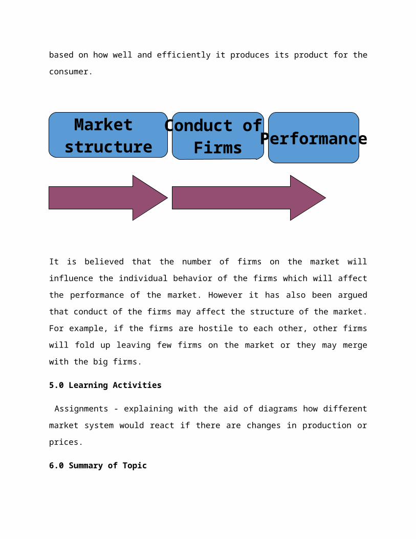
and unbiased. Efficient market hypothesis is the idea that information is quickly and efficiently incorporated into asset prices at any point in time, so that old information cannot be used to foretell future price movements. Consequently, three versions of EMH are being distinguished depends on the level of available information.

The weak form EMH stipulates that current asset prices already reflect past price and volume information. The information contained in the past sequence of prices of a security is fully reflected in the current market price of that security. It is named weak form because the security prices are the most publicly and easily accessible pieces of information. It implies that no one should be able to outperform the market using something that "everybody else knows". Yet, there are still numbers of financial researchers who are studying the past stock price series and trading volume data in attempt to generate profit. This technique is so called technical analysis that is asserted by EMH as useless for predicting future price changes.

The semi strong form EMH states that all publicly available information is similarly already incorporated into asset prices. In another word, all publicly available information is fully reflected in a security's current market price. The public information stated not only past prices but also data reported in a company's financial statements, company's announcement, economic factors and others. It also implies that no one should be able to outperform the market using something that "everybody else knows". This indicates that a company's financial statements are of no help in forecasting future price movements and securing high investment returns.

The strong form EMH stipulates that private information or insider information too, is quickly incorporated by market prices and therefore cannot be used to reap abnormal trading profits. Thus, all information, whether public or private, is fully reflected in a security's current market price. That's mean, even the company's management (insider) are not able to make gains from inside information they hold. They are not able to take the advantages to profit from information such as take over decision which has been made ten minutes ago. The rationale behind to support is that the market anticipates in an unbiased manner, future development and therefore information has been incorporated and evaluated into market price in much more objective and informative way than insiders.

The random walk model of asset prices is an extension of the EMH, as are the notions that the market cannot be consistently beaten, arbitrage is impossible, and "free lunches" are generally unavailable.

2.2) The implications of the EMH for optimal investment strategies

The EMH has implied that no one can outperform the market either with security selection or with market timing. Thus, it carries huge negative implications for many investment strategies. Generally, the impact of EMH can be viewed from two different perspectives:

i) Investors perspective:

Technical analysis uses past patterns of price and the volume of trading as the basis for predicting future prices. The random-walk evidence suggests that prices of securities are affected by news. Favourable news will push up the price and vice versa. It is therefore appropriate to question the value of technical analysis as a means of choosing security investments. Fundamentals analysis involves using market information to determine the intrinsic value of securities in order to identify those securities that are undervalued. However semi strong form market efficiency suggests that fundamentals analysis cannot be used to outperform the market. In an efficient market, equity research and valuation would be a costly task that provided no benefits. The odds of finding an undervalued stock should be random (50/50). Most of the time, the benefits from information collection and equity research would not cover the costs of doing the research.

For optimal investment strategies, investors are suggested should follow a passive investment strategy, which makes no attempt to beat the market. Investors should not select securities randomly according to their risk aversion or the tax positions. This does not means that there is no portfolio management. In an efficient market, it would be superior strategy to have a randomly diversifying across securities, carrying little or no information cost and minimal execution costs in order to optimise the returns. There would be no value added by portfolio managers and investment strategists. An inflexible buy-and-hold policy is not optimal for matching the investor's desired risk level. In addition, the portfolio manager must choose a portfolio that is geared toward the time horizon and risks profile of the investor.

ii) Financial managers’ perspective

Managers need to keep in mind that markets would under react or over react to information, the company's share price will reflect the information about their announcements (information). The historical share price record can be used as a measure of company performance and management bear responsibility for it. When share are under priced, managers should avoid issuing new shares. This will only worsen the situation. In normal circumstances, market efficiency theory provides useful insight into price behaviour. Generally, it can be concluded that investors should only expect a normal rate of return while company should expect to receive the fair value for the securities they issue.

An investment theory that states it is impossible to "beat the market" because stock market efficiency causes existing share prices to always incorporate and reflect all relevant information. According to the EMH, stocks always trade at their fair value on stock exchanges, making it impossible for investors to either purchase undervalued stocks or sell stocks for inflated prices. As such, it should be impossible to outperform the overall market through expert stock selection or market timing, and that the only way an investor can possibly obtain higher returns is by purchasing riskier investments

Although it is a cornerstone of modern financial theory, the EMH is highly controversial and often disputed. Believers argue it is pointless to search for undervalued stocks or to try to predict trends in the market through either fundamental or technical analysis.

Meanwhile, while academics point to a large body of evidence in support of EMH, an equal amount of dissension also exists. For example, investors, such as Warren Buffett have consistently beaten the market over long periods of time, which by definition is impossible according to the EMH. Detractors of the EMH also point to events, such as the 1987 stock market crash when the Dow Jones Industrial Average (DJIA) fell by over 20% in a single day, as evidence that stock prices can seriously deviate from their fair values

When money is put into the stock market, it is done with the aim of generating a return on the capital invested. Many investors try not only to make a profitable return, but also to outperform, or beat, the market.

However, market efficiency - championed in the efficient market hypothesis (EMH) formulated by Eugene Fama in 1970, suggests that at any given time, prices fully reflect all available information on a particular stock and/or market. Thus, according to the EMH, no investor has an advantage in predicting a return on a stock price because no one has access to information not already available to everyone else. (To read more on behavioral finance, see Taking A Chance On Behavioral Finance, Understanding Investor Behavior and Mad Money ... Mad Market?)

The Effect of Efficiency: Non-Predictability

The nature of information does not have to be limited to financial news and research alone; indeed, information about political, economic and social events, combined with how investors perceive such information, whether true or rumored, will be reflected in the stock price. According to EMH, as prices respond only to information available in the market, and, because all market participants are privy to the same information, no one will have the ability to out-profit anyone else. In efficient markets, prices become not predictable but random, so no investment pattern can be discerned. A planned approach to investment, therefore, cannot be

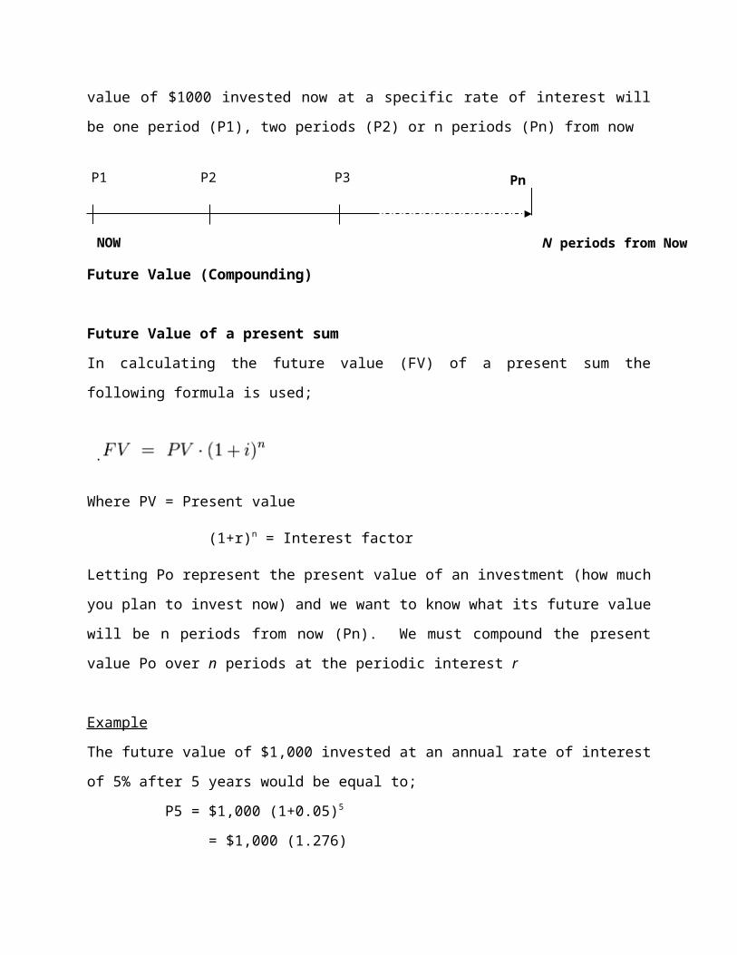
successful.This "random walk" of prices, commonly spoken about in the EMH school of thought, results in the failure of any investment strategy that aims to beat the market consistently. In fact, the EMH suggests that given the transaction costs involved in portfolio management, it would be more profitable for an investor to put his or her money into an index fund.

Anomalies: The Challenge to Efficiency

In the real world of investment, however, there are obvious arguments against the EMH. There are investors who have beaten the market - Warren Buffett, whose investment strategy focuses on undervalued stocks, made millions and set an example for numerous followers. There are portfolio managers who have better track records than others, and there are investment houses with more renowned research analysis than others. So how can performance be random when people are clearly profiting from and beating the market?

Counter arguments to the EMH state that consistent patterns are present. Here are some examples of some of the predictable anomalies thrown in the face of the EMH: the January effect is a pattern that shows higher returns tend to be earned in the first month of the year; "blue Monday on Wall Street" is a saying that discourages buying on Friday afternoon and Monday morning because of the weekend effect, the tendency for prices to be higher on the day before and after the weekend than during the rest of the week.

Studies in behavioral finance, which look into the effects of investor psychology on stock prices, also reveal that there are some predictable patterns in the stock market. Investors tend to buy undervalued stocks and sell overvalued stocks and, in a market of many participants, the result can be anything but efficient.

Paul Krugman, MIT economics professor, suggests that because of the mass mentality of the trendy, short-term shareholder, investors pull in and out of the latest and hottest stocks. This results in stock prices being distorted and the market being inefficient. So prices no longer reflect all available information in the market. Prices are instead being manipulated by profit seekers.

The EMH Response

The EMH does not dismiss the possibility of anomalies in the market that result in the generation of superior profits. In fact, market efficiency does not require prices to be equal to fair value all of the time. Prices may be over- or undervalued only in random occurrences, so they eventually revert back to their mean values. As such, because the deviations from a stock's

fair price are in themselves random, investment strategies that result in beating the market cannot be consistent phenomena.

Furthermore, the hypothesis argues that an investor who outperforms the market does so not out of skill but out of luck. EMH followers say this is due to the laws of probability: at any given time in a market with a large number of investors, some will outperform while other will remain average.

How Does a Market Become Efficient?

In order for a market to become efficient, investors must perceive that a market is inefficient and possible to beat. Ironically, investment strategies intended to take advantage of inefficiencies are actually the fuel that keeps a market efficient.

A market has to be large and liquid. Information has to be widely available in terms of accessibility and cost and released to investors at more or less the same time. Transaction costs have to be cheaper than the expected profits of an investment strategy. Investors must also have enough funds to take advantage of inefficiency until, according to the EMH, it disappears again. Most importantly, an investor has to believe that she or he can outperform the market.

Degrees of Efficiency

Accepting the EMH in its purest form may be difficult; however, there are three identified classifications of the EMH, which are aimed at reflecting the degree to which it can be applied to markets.

1. Strong efficiency - This is the strongest version, which states that all information in a market, whether public or private, is accounted for in a stock price. Not even insider information could give an investor an advantage

2. Semi-strong efficiency - This form of EMH implies that all public information is calculated into a stock's current share price. Neither fundamental nor technical analysis can be used to achieve superior gains

3. Weak efficiency - This type of EMH claims that all past prices of a stock are reflected in today's stock price. Therefore, technical analysis cannot be used to predict and beat a market.

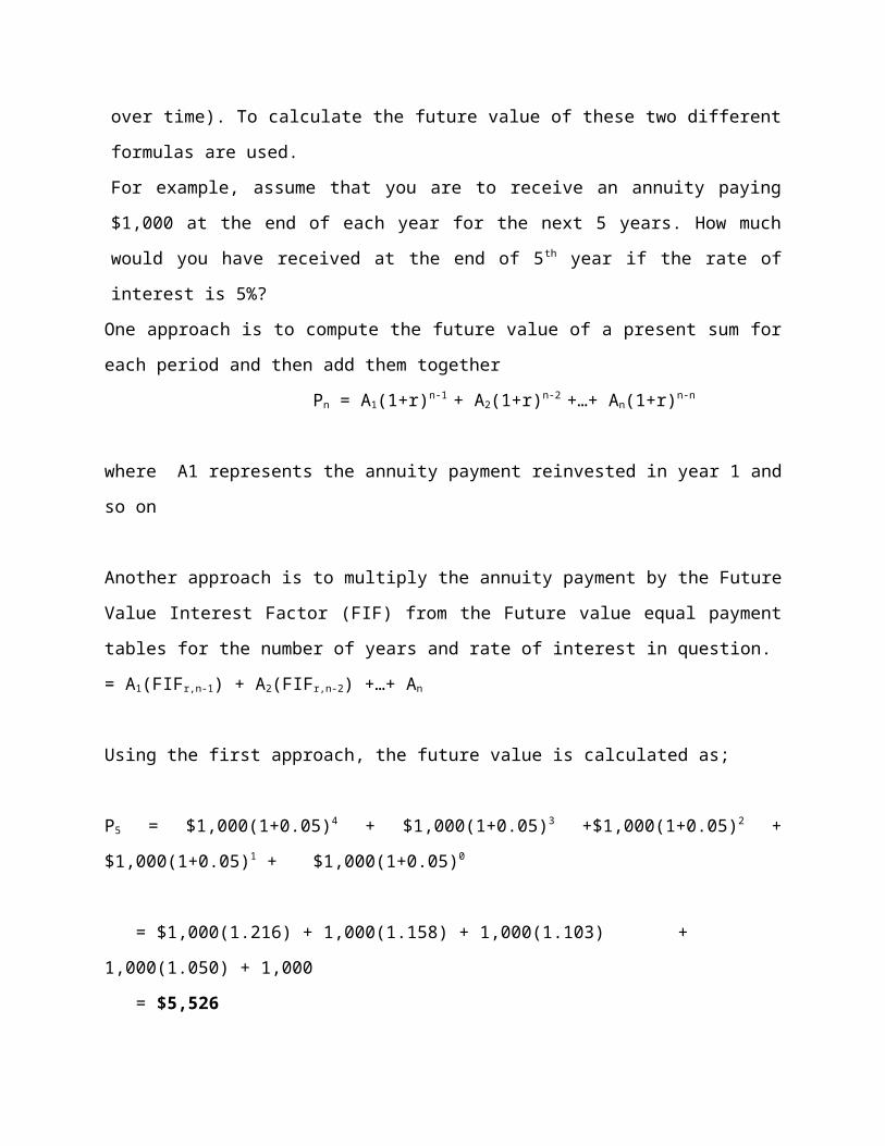
Random Walk Theory

The theory that stock price changes have the same distribution and are independent of each other, so the past movement or trend of a stock price or market cannot be used to predict its future movement.

In short, this is the idea that stocks take a random and unpredictable path. A follower of the random walk theory believes it's impossible to outperform the market without assuming additional risk. Critics of the theory, however, contend that stocks do maintain price trends over time - in other words, that it is possible to outperform the market by carefully selecting entry and exit points for equity investments.

ConclusionEMH propagandists will state that profit seekers will, in practice, exploit whatever abnormally exists until it disappears. In instances such as the January effect (a predictable pattern of price movements), large transactions costs will most likely outweigh the benefits of trying to take advantage of such a trend.

In the real world, markets cannot be absolutely efficient or wholly inefficient. It might be reasonable to see markets as essentially a mixture of both, wherein daily decisions and events cannot always be reflected immediately into a market. If all participants were to believe that the market is efficient, no one would seek extraordinary profits, which is the force that keeps the wheels of the market turning.

In the age of information technology (IT), however, markets all over the world are gaining greater efficiency. IT allows for a more effective, faster means to disseminate information, and electronic trading allows for prices to adjust more quickly to news entering the market. However, while the pace at which we receive information and make transactions quickens, IT also restricts the time it takes to verify the information used to make a trade. Thus, IT may inadvertently result in less efficiency if the quality of the information we use no longer allows us to make profit-generating decisions.

Learning Activities

Assignments, discussions

Summary of Topic

Further Reading Materials

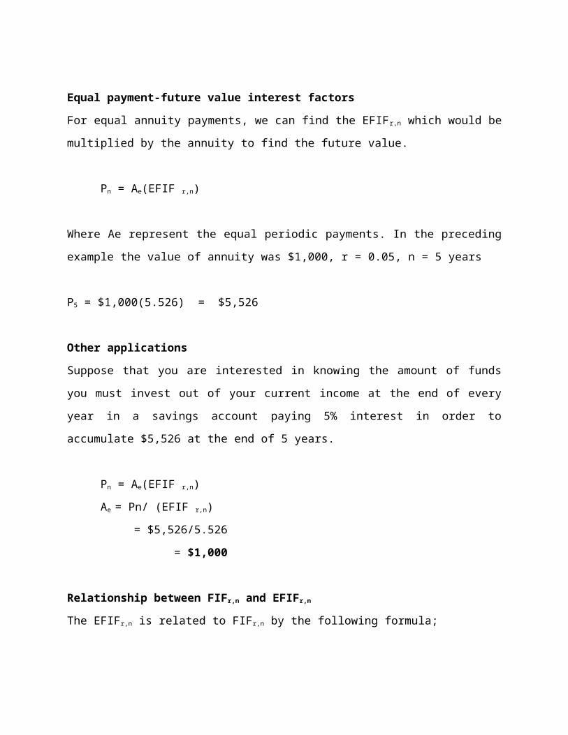
• Fama, E. F., (1970) "Efficient Capital Markets: A Review of Theory and Empirical Work,"

Journal of Finance, 25:2, 383-417.

• Jonathan, C., Tomas, J., and Gershon M., "The Efficient Markets Hypothesis",

http://comp.uark.edu/~tjandik/papers/emh.pdf

• Richard, P., and Bill, N., (1999) Corporate Finance and Investment Decision and

Strategies, (3rd edn), England, Pearson Education Limited, Chapter 2.

Useful Links

www.egwald.ca/economics/index

www.regulationbodyofknowledge.org/chapter2/narrative/1/

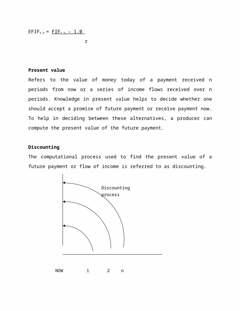
Topic 8: Welfare Economics

In this topic you will learn how resources are allocated equitably within the society so that no person is made worse off. You will learn about economic equilibrium and the welfare effects of changes in economic equilibrium. That is, this course is about economic markets, how they work and don’t work, and how exogenous factors like government policy or technological change affect the welfare of economic agents. This course will introduce you to the formal theory of how and why economic markets work well or do not work well in the absence of outside intervention. The course will also introduce you to methods used to measure the effects of any such intervention on the welfare of economic agents.

Learning Outcomes

Upon completion of this lesson you will be able to;

Explain the rationale behind welfare economics

Describe conditions that lead to inefficient allocation of resources

Key Terms: Pareto Optimality, Kaldor-Hicks efficiency, Gini Coefficient, Social welfare

1.0 Introduction to Welfare economics

This is a branch of economics that focuses on the optimal allocation of resources and goods and how this affects social welfare. Welfare economics analyzes the total good or welfare that is achieved at a current state as well as how it is distributed. This relates to the study of income distribution and how it affects the common good. Welfare economics is a subjective study that may assign units of welfare or utility in order to create models that measure the improvements to individuals based on their personal scales.

It is a branch of economics that uses microeconomic techniques to evaluate economic well-being, especially relative to competitive general equilibrium within an economy as to economic efficiency and the resulting income distribution associated with it. It analyzes social welfare, however measured, in terms of economic activities of the individuals that comprise the theoretical society considered. As such, individuals, with associated economic activities, are the basic units for aggregating to social welfare, whether of a group, a community, or a society, and there is no "social welfare" apart from the "welfare" associated with its individual units.

Welfare economics typically takes individual preferences as given and stipulates a welfare improvement in Pareto efficiency terms from social state A to social state B if at least one person prefers B and no one else opposes it. There is no requirement of a unique quantitative measure of the welfare improvement implied by this. Another aspect of welfare treats income/goods distribution, including equality, as a further dimension of welfare.

Social welfare refers to the overall welfare of society. With sufficiently strong assumptions, it can be specified as the summation of the welfare of all the individuals in the society. Welfare may be measured either cardinally in terms of "utils" or dollars, or measured ordinally in terms of Pareto efficiency. The cardinal method in "utils" is seldom used in pure theory today because of aggregation problems that make the meaning of the method doubtful, except on widely challenged underlying assumptions. In applied welfare economics, such as in cost-benefit analysis, money-value estimates are often used, particularly where income-distribution effects are factored into the analysis or seem unlikely to undercut the analysis.

Since the early 1980s economists have been interested in a number of new approaches and issues in welfare economics. The capabilities approach to welfare argues that what people are free to do or be should also be included in welfare assessments and the approach has been particularly influential in development policy circles where the emphasis on multi-dimensionality and freedom has shaped the evolution of the Human Development Index.

Economists have also been interested in using life satisfaction to measure what Kahneman and colleagues call experienced utility.

What follows, for the most part, therefore refers to a particular approach to welfare economics, possibly best referred to as 'neo-classical' or 'traditional' welfare economics.

Other classifying terms or problems in welfare economics include externalities, equity, justice, inequality, and altruism.

2.0 Approaches to studying welfare economics

There are two mainstream approaches to welfare economics: the early Neoclassical approach and the New welfare economics approach.

The early Neoclassical approach was developed by Edgeworth, Sidgwick, Marshall, and Pigou. It assumes that:

Utility is cardinal, that is, scale-measurable by observation or judgment. Preferences are exogenously given and stable.

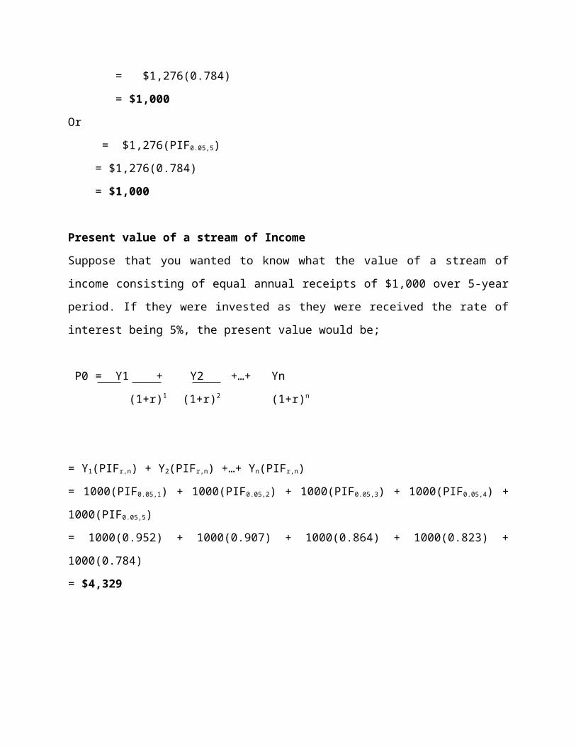
Additional consumption provides smaller and smaller increases in utility (diminishing marginal utility).

All individuals have interpersonally comparable utility functions (an assumption that Edgeworth avoided in his Mathematical 'Psychics).

With these assumptions, it is possible to construct a social welfare function simply by summing all the individual utility functions.

The New Welfare Economics approach is based on the work of Pareto, Hicks, and Kaldor. It explicitly recognizes the differences between the efficiency aspect of the discipline and the distribution aspect and treats them differently. Questions of efficiency are assessed with criteria such as Pareto efficiency and the Kaldor-Hicks compensation tests, while questions of income distribution are covered in social welfare function specification. Further, efficiency dispenses with cardinal measures of utility, replacing it with ordinal utility, which merely ranks commodity bundles, such as represented by an indifference-curve map is adequate for this analysis.

3.0 Pareto efficiency

Situations are considered to have distributive efficiency when goods are distributed to the people who can gain the most utility from them.

Many economists use Pareto efficiency as their efficiency goal. According to this measure of social welfare, a situation is optimal only if no individuals can be made better off without making someone else worse off. An economic system that is not Pareto efficient implies that a certain change in allocation of goods (for example) may result in some individuals being made "better off" with no individual being made worse off, and therefore can be made more Pareto efficient through a Pareto improvement. Here 'better off' is often interpreted as "put in a preferred position." It is commonly accepted that outcomes that are not Pareto efficient are to be avoided, and therefore Pareto efficiency is an important criterion for evaluating economic systems and public policies. If economic allocation in any system is not Pareto efficient, there is potential for a Pareto improvement—an increase in Pareto efficiency: through reallocation, improvements to at least one participant's well-being can be made without reducing any other participant's well-being If economic allocation in any system is not Pareto efficient, there is potential for a Pareto improvement—an increase in Pareto efficiency: through reallocation, improvements to at least one participant's well-being can be made without reducing any other participant's well-being

This ideal state of affairs can only come about if four criteria are met:

The marginal rates of substitution in consumption are identical for all consumers. This occurs when no consumer can be made better off without making others worse off.

The marginal rate of transformation in production is identical for all products. This occurs when it is impossible to increase the production of any good without reducing the production of other goods.

The marginal resource cost is equal to the marginal revenue product for all production processes. This takes place when marginal physical product of a factor must be the same for all firms producing a good.

The marginal rates of substitution in consumption are equal to the marginal rates of transformation in production, such as where production processes must match consumer wants.

There are a number of conditions that, most economists agree, may lead to inefficiency. They include:

Imperfect market structures, such as a monopoly, monopsony, oligopoly, oligopsony, and monopolistic competition.

Factor allocation inefficiencies in production theory basics.

Market failures and externalities; there is also social cost.

Price discrimination and price skimming.

Asymmetric information, principal-agent problems.

Long run declining average costs in a natural monopoly.

Certain types of taxes and tariffs.

To determine whether an activity is moving the economy towards Pareto efficiency, two compensation tests have been developed. Any change usually makes some people better off while making others worse off, so these tests ask what would happen if the winners were to compensate the losers. Using the Kaldor criterion, an activity will contribute to Pareto optimality if the maximum amount the gainers are prepared to pay is greater than the minimum amount that the losers are prepared to accept. Under the Hicks criterion, an activity will contribute to Pareto optimality if the maximum amount the losers are prepared to offer to the gainers in order to prevent the change is less than the minimum amount the gainers are prepared to accept as a bribe to forgo the change. The Hicks compensation test is from the

losers' point of view, while the Kaldor compensation test is from the gainers' point of view. If both conditions are satisfied, both gainers and losers will agree that the proposed activity will move the economy toward Pareto optimality. This is referred to as Kaldor-Hicks efficiency or the Scitovsky criterion.

In real-world practice, the compensation principle often appealed to is hypothetical. That is, for the alleged Pareto improvement (say from public regulation of the monopolist or removal of tariffs) some losers are not (fully) compensated. The change thus results in distribution effects in addition to any Pareto improvement that might have taken place. The theory of hypothetical compensation is part of Kaldor-Hicks efficiency, also called Potential Pareto Criterion.

Under certain idealized conditions, it can be shown that a system of free markets will lead to a Pareto efficient outcome. This is called the first welfare theorem

4.0 Pareto frontier

Fig Example of a Pareto frontier.

The boxed points represent feasible choices, and smaller values are preferred to larger ones. Point C is not on the Pareto Frontier because it is dominated by both point A and point B. Points A and B are not strictly dominated by any other, and hence do lie on the frontier.

Given a set of choices and a way of valuing them, the Pareto frontier or Pareto set is the set of choices that are Pareto efficient. The Pareto frontier is particularly useful in engineering: by restricting attention to the set of choices that are Pareto-efficient, a designer can make tradeoffs within this set, rather than considering the full range of every parameter.

The Pareto frontier is defined formally as follows.

Consider a design space with n real parameters, and for each design space point there are m

different criteria by which to judge that point. Let be the function which assigns, to each design space point x, a criteria space point f(x). This represents the way of valuing the designs. Now, it may be that some designs are infeasible; so let X be a set of feasible designs in , which must be a compact set. Then the set which represents the feasible criterion points is f(X), the image of the set X under the action of f. Call this image Y.

Now construct the Pareto frontier as a subset of Y, the feasible criterion points. It can be assumed that the preferable values of each criterion parameter are the lesser ones, thus minimizing each dimension of the criterion vector. Then compare criterion vectors as follows: One criterion vector y strictly dominates (or "is preferred to") a vector y* if each parameter of y is no greater than the corresponding parameter of y* and at least one parameter is strictly less: that is, for each i and for some i. This is written as to mean that y strictly dominates y*. Then the Pareto frontier is the set of points from Y that are not strictly dominated by another point in Y.

Formally, this defines a partial order on Y, namely the product order on (more precisely, the induced order on Y as a subset of ), and the Pareto frontier is the set of maximal elements with respect to this order.

Algorithms for computing the Pareto frontier of a finite set of alternatives have been studied in computer science, being sometimes referred to as the maximum vector problem or the skyline query

5.0 Income distribution

There are many combinations of consumer utility, production mixes, and factor input combinations consistent with efficiency. In fact, there are an infinity of consumer and production equilibria that yield Pareto optimal results. There are as many optimal as there are points on the aggregate production possibilities frontier. Hence, Pareto efficiency is a necessary, but not a sufficient condition for social welfare. Each Pareto optimum corresponds to a different income distribution in the economy. Some may involve great inequalities of income. So how do we decide which Pareto optimum is most desirable? This decision is made, either tacitly or overtly, when we specify the social welfare function. This function embodies value judgements about interpersonal utility. The social welfare function is a way of mathematically stating the relative importance of the individuals that comprise society.

A utilitarian welfare function (also called a Benthamite welfare function) sums the utility of each individual in order to obtain society's overall welfare. All people are treated the same,

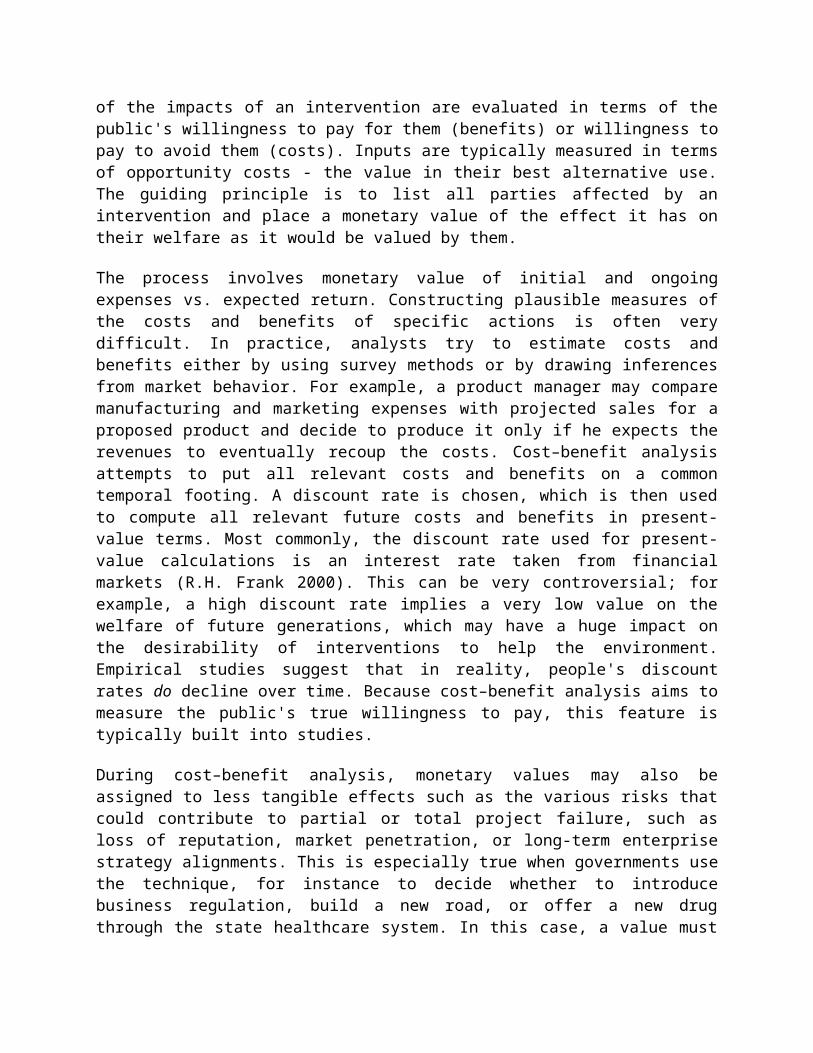
regardless of their initial level of utility. One extra unit of utility for a starving person is not seen to be of any greater value than an extra unit of utility for a millionaire. At the other extreme is the Max-Min, or Rawlsian John Rawls utility function (Stiglitz, 2000, p102). According to the Max-Min criterion, welfare is maximized when the utility of those society members that have the least is the greatest. No economic activity will increase social welfare unless it improves the position of the society member that is the worst off. Most economists specify social welfare functions that are intermediate between these two extremes.

The social welfare function is typically translated into social indifference curves so that they can be used in the same graphic space as the other functions that they interact with. A utilitarian social indifference curve is linear and downward sloping to the right. The Max-Min social indifference curve takes the shape of two straight lines joined so as they form a 90 degree angle. A social indifference curve drawn from an intermediate social welfare function is a curve that slopes downward to the right.

Utilitarian social indifference curve

The intermediate form of social indifference curve can be interpreted as showing that as inequality increases, a larger improvement in the utility of relatively rich individuals is needed to compensate for the loss in utility of relatively poor individuals.

A crude social welfare function can be constructed by measuring the subjective dollar value of goods and services distributed to participants in the economy.

5.1 Gini Coefficient

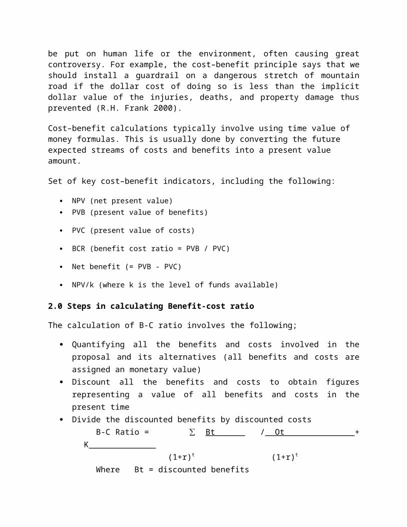
The Gini coefficient is usually defined mathematically based on the Lorenz curve, which plots the proportion of the total income of the population (y axis) that is cumulatively earned by the bottom x% of the population (see diagram). The line at 45 degrees thus represents perfect equality of incomes. The Gini coefficient can then be thought of as the ratio of the area that lies between the line of equality and the Lorenz curve (marked 'A' in the diagram) over the total area under the line of equality (marked 'A' and 'B' in the diagram); i.e., G=A/(A+B).

Graphical representation of the Gini coefficient.

The graph shows that the Gini is equal to the area marked 'A' divided by the sum of the areas marked 'A' and 'B' (that is, Gini = A/(A+B)). It is also equal to 2*A, as A+B = 0.5 (since the axes scale from 0 to 1. The Gini coefficient can range from 0 to 1; it is sometimes multiplied by 100 to range between 0 and 100. A low Gini coefficient indicates a more equal distribution, with 0 corresponding to complete equality, while higher Gini coefficients indicate more unequal distribution, with 1 corresponding to complete inequality. To be validly computed, no negative goods can be distributed. Thus, if the Gini coefficient is being used to describe household income inequality, then no household can have a negative income. When used as a measure of income inequality, the most unequal society will be one in which a single person receives 100% of the total income and the remaining people receive none (G=1); and the most equal society will be one in which every person receives the same income (G=0).

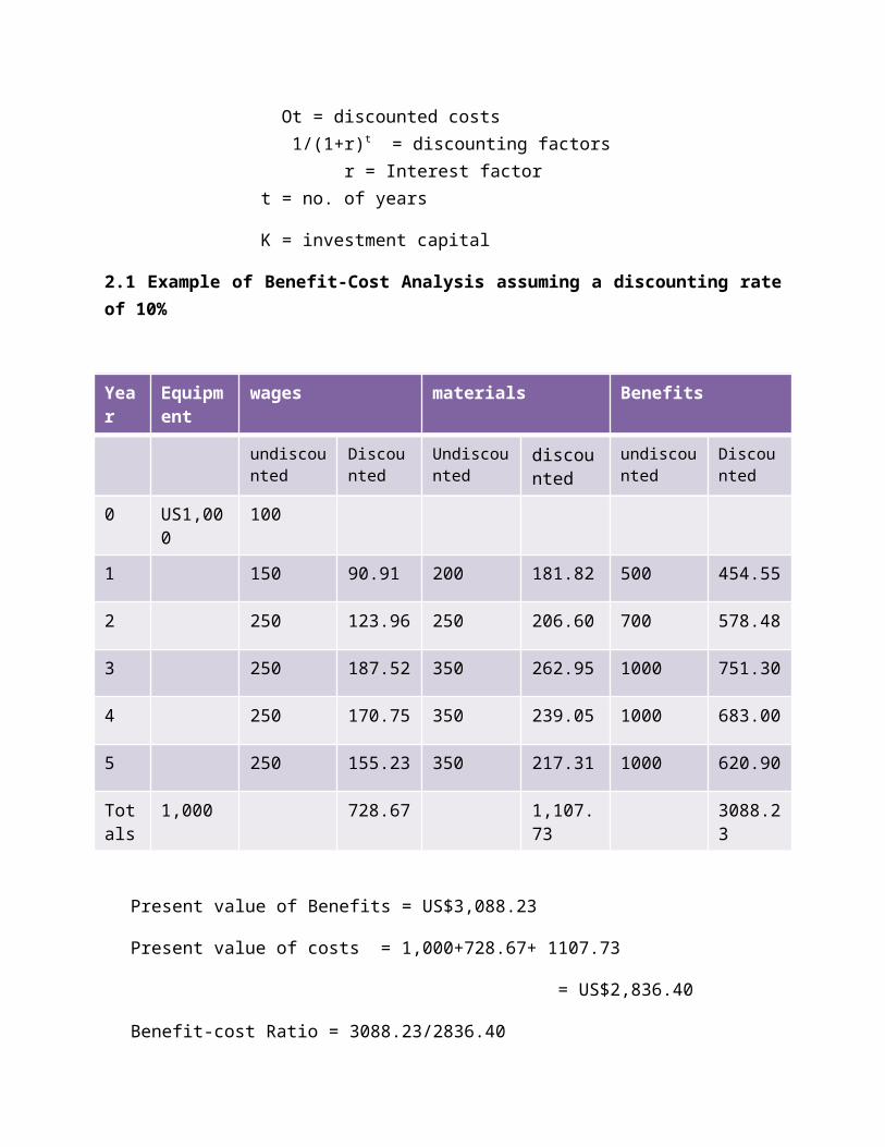
Some find it more intuitive (and it is mathematically equivalent) to think of the Gini coefficient as half of the relative mean difference. The mean difference is the average absolute difference between two items selected randomly from a population, and the relative mean difference is the mean difference divided by the average, to normalize for scale.

5.1.1 Calculation

The Gini index is defined as a ratio of the areas on the Lorenz curve diagram. If the area between the line of perfect equality and the Lorenz curve is A, and the area under the Lorenz curve is B, then the Gini index is A/(A+B). Since A+B = 0.5, the Gini index, G = A/(0.5) = 2A = 1-2B. If the Lorenz curve is represented by the function Y = L(X), the value of B can be found with integration and:

In some cases, this equation can be applied to calculate the Gini coefficient without direct reference to the Lorenz curve. For example:

For a population uniform on the values yi, i = 1 to n, indexed in non-decreasing order ( yi

≤ yi+1):

This may be simplified to:

For a discrete probability function f(y), where yi, i = 1 to n, are the points with nonzero probabilities and which are indexed in increasing order ( yi < yi+1):

where

and

For a cumulative distribution function F(y) that is piecewise differentiable, has a mean μ, and is zero for all negative values of y:

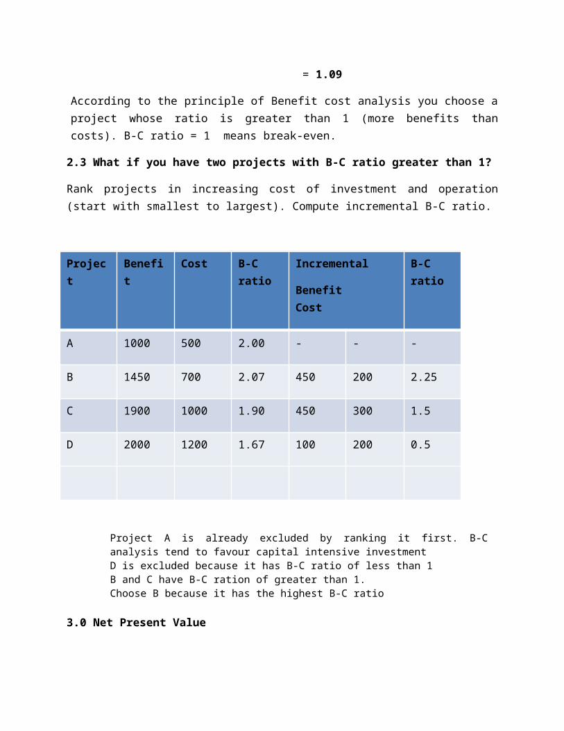
Since the Gini coefficient is half the relative mean difference, it can also be calculated using formulas for the relative mean difference. For a random sample S consisting of values yi, i = 1 to n, that are indexed in non-decreasing order ( yi ≤ yi+1), the statistic:

is a consistent estimator of the population Gini coefficient, but is not, in general, unbiased. Like, G, G(S) has a simpler form:

.

There does not exist a sample statistic that is in general an unbiased estimator of the population Gini coefficient, like the relative mean difference.

Sometimes the entire Lorenz curve is not known, and only values at certain intervals are given. In that case, the Gini coefficient can be approximated by using various techniques for interpolating the missing values of the Lorenz curve. If ( X k , Yk ) are the known points on the Lorenz curve, with the X k indexed in increasing order ( X k - 1 < X k ), so that:

Xk is the cumulated proportion of the population variable, for k = 0,...,n, with X 0 = 0, Xn = 1.

Yk is the cumulated proportion of the income variable, for k = 0,...,n, with Y0 = 0, Yn = 1.

Yk should be indexed in non-decreasing order (Yk>Yk-1)

If the Lorenz curve is approximated on each interval as a line between consecutive points, then the area B can be approximated with trapezoids and:

is the resulting approximation for G. More accurate results can be obtained using other methods to approximate the area B, such as approximating the Lorenz curve with a quadratic function across pairs of intervals, or building an appropriately smooth approximation to the underlying distribution function that matches the known data. If the population mean and boundary values for each interval are also known, these can also often be used to improve the accuracy of the approximation.

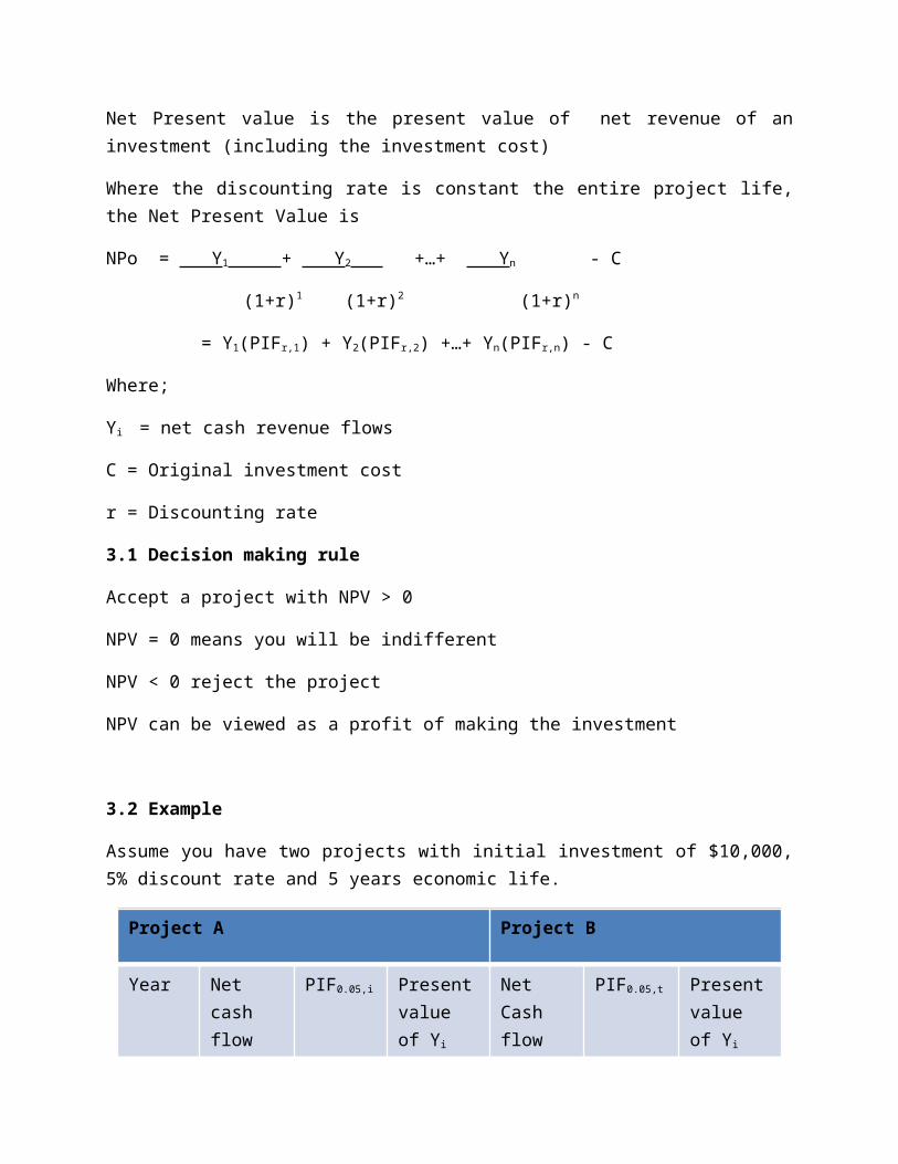
The Gini coefficient calculated from a sample is a statistic and its standard error, or confidence intervals for the population Gini coefficient, should be reported. These can be calculated using bootstrap techniques but those proposed have been mathematically complicated and computationally onerous even in an era of fast computers. Ogwang (2000) made the process more efficient by setting up a “trick regression model” in which the incomes in the sample are ranked with the lowest income being allocated rank 1. The model then expresses the rank (dependent variable) as the sum of a constant A and a normal error term whose variance is inversely proportional to yk;

Ogwang showed that G can be expressed as a function of the weighted least squares estimate of the constant A and that this can be used to speed up the calculation of the jackknife estimate for the standard error. Giles (2004) argued that the standard error of the estimate of A can be used to derive that of the estimate of G directly without using a jackknife at all. This method only requires the use of ordinary least squares regression after ordering the sample data. The results compare favorably with the estimates from the jackknife with agreement improving with increasing sample size. The paper describing this method can be found here: http://web.uvic.ca/econ/ewp0202.pdf

However it has since been argued that this is dependent on the model’s assumptions about the error distributions (Ogwang 2004) and the independence of error terms (Reza & Gastwirth 2006) and that these assumptions are often not valid for real data sets. It may therefore be better to stick with jackknife methods such as those proposed by Yitzhaki (1991) and Karagiannis and Kovacevic (2000). The debate continues.

The Gini coefficient can be calculated if you know the mean of a distribution, the number of people (or percentiles), and the income of each person (or percentile). Princeton development economist Angus Deaton (1997, 139) simplified the Gini calculation to one easy formula:

where u is mean income of the population, P i is the income rank P of person i, with income X, such that the richest person receives a rank of 1 and the poorest a rank of N. This effectively gives higher weight to poorer people in the income distribution, which allows the Gini to meet the Transfer Principle.

5.1.2 Advantages of Gini coefficient as a measure of inequality

The Gini coefficient's main advantage is that it is a measure of inequality by means of a ratio analysis, rather than a variable unrepresentative of most of the population, such as per capita income or gross domestic product.

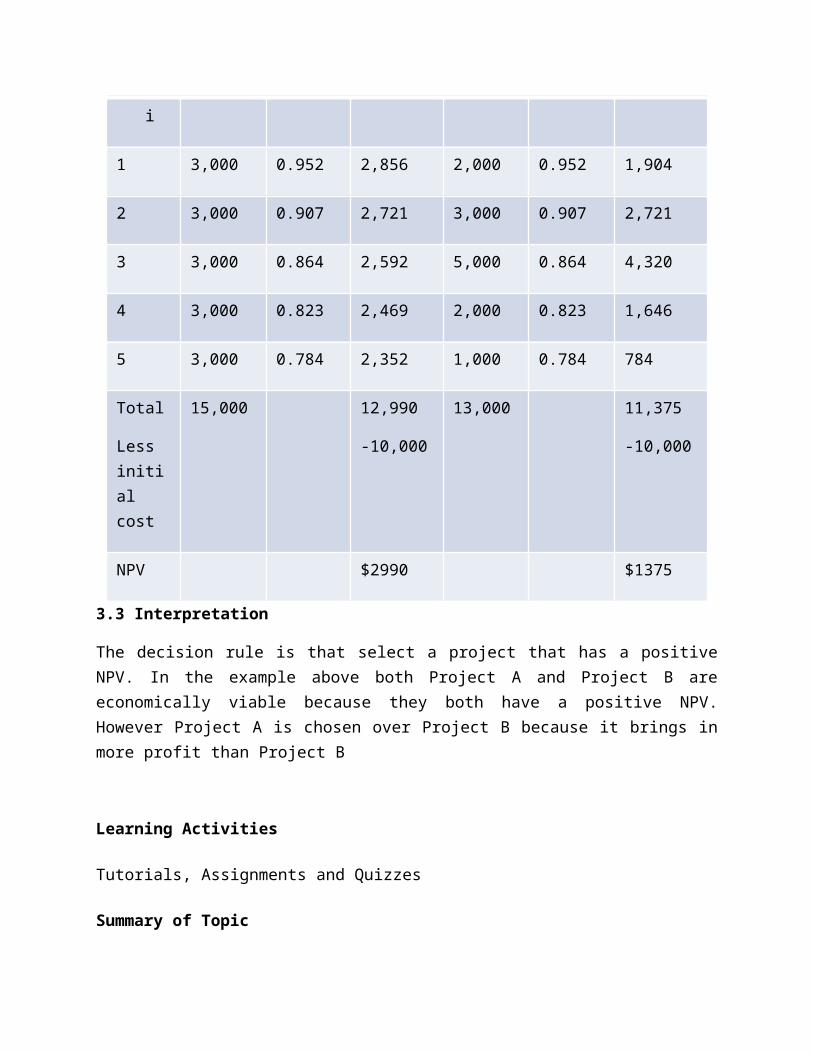
It can be used to compare income distributions across different population sectors as well as countries, for example the Gini coefficient for urban areas differs from that of rural areas in many countries (though the United States' urban and rural Gini coefficients are nearly identical).

It is sufficiently simple that it can be compared across countries and be easily interpreted. GDP statistics are often criticized as they do not represent changes for the whole population; the Gini coefficient demonstrates how income has changed for poor and rich. If the Gini coefficient is rising as well as GDP, poverty may not be improving for the majority of the population.

The Gini coefficient can be used to indicate how the distribution of income has changed within a country over a period of time, thus it is possible to see if inequality is increasing or decreasing.

The Gini coefficient satisfies four important principles:

Anonymity: it does not matter who the high and low earners are. Scale independence: the Gini coefficient does not consider the size of the economy, the

way it is measured, or whether it is a rich or poor country on average.

Population independence: it does not matter how large the population of the country is.

Transfer principle: if income (less than half of the difference), is transferred from a rich person to a poor person the resulting distribution is more equal.

5.1.2 Disadvantages of Gini coefficient as a measure of inequality

While the Gini coefficient measures inequality of income, it does not measure inequality of opportunity. For example, some countries may have a social class structure that may present barriers to upward mobility; this is not reflected in their Gini coefficients.

If two countries have the same Gini coefficient but one is rich and the other is poor, it can be seen to measure two different things. In a poor country it measures the inequality in material life quality while in a rich country it measures the distribution of luxury beyond the basic necessities.

The Gini coefficient of different sets of people cannot be averaged to obtain the Gini coefficient of all the people in the sets: if a Gini coefficient were to be calculated for each person it would always be zero. For a large, economically diverse country, a much higher coefficient will be calculated for the country as a whole than will be calculated for each of its regions. (The coefficient is usually applied to measurable nominal income rather than local purchasing power, tending to increase the calculated coefficient across larger areas.)

The Lorenz curve may understate the actual amount of inequality if richer households are able to use income more efficiently than lower income households or vice versa. From another point

of view, measured inequality may be the result of more or less efficient use of household incomes.

Economies with similar incomes and Gini coefficients can still have very different income distributions. (This is true for any single measure of a distribution.) This is because the Lorenz curves can have different shapes and yet still yield the same Gini coefficient. For example, consider a society where half of individuals had no income and the other half shared all the income equally (i.e. whose Lorenz curve is linear from (0,0) to (0.5,0) and then linear to (1,1)). As is easily calculated, this society has Gini coefficient 0.5 -- the same as that of a society in which 75% of people equally shared 25% of income while the remaining 25% equally shared 75% (i.e. whose Lorenz curve is linear from (0,0) to (0.75,0.25) and then linear to (1,1)).

It measures current income rather than lifetime income. A society in which everyone earned the same over a lifetime would appear unequal because of people at different stages in their life. However, Gini coefficient can also be calculated for any kind of single-variable distribution, e.g. for wealth.

Gini coefficients do include investment income; however, the Gini coefficient based on net income does not accurately reflect differences in wealth—a possible source of misinterpretation. For example, Sweden has a low Gini coefficient for income distribution but a significantly higher Gini coefficient for wealth (for instance 77% of the share value owned by households is held by just 5% of Swedish shareholding households). [14] In other words, the Gini income coefficient should not be interpreted as measuring effective egalitarianism.

Too often only the Gini coefficient is quoted without describing the proportions of the quantiles used for measurement. As with other inequality coefficients, the Gini coefficient is influenced by the granularity of the measurements. For example, five 20% quantiles (low granularity) will usually yield a lower Gini coefficient than twenty 5% quantiles (high granularity) taken from the same distribution. This is an often encountered problem with measurements.

Care should be taken in using the Gini coefficient as a measure of egalitarianism, as it is properly a measure of income dispersion. For example, if two equally egalitarian countries pursue different immigration policies, the country accepting higher proportion of low-income or impoverished migrants will be assessed as less equal (gain a higher Gini coefficient).

The Gini coefficient is a point-estimate of equality at a certain time, hence it ignores life-span changes in income. Typically, increases in the proportion of young or old members of a society will drive apparent changes in equality. Because of this, factors such as age distribution within a population and mobility within income classes can create the appearance of differential equality when none exist taking into account demographic effects. Thus a given economy may have a higher Gini coefficient at any one point in time compared to another, while the Gini coefficient calculated over individuals' lifetime income is actually lower than the apparently more equal (at a given point in time) economy's.[15] Essentially, what matters is not just inequality in any particular year, but the composition of the distribution over time.

6.0 Learning Activities

Assignments, Questions, discussion, and critique

7.0 Summary of Topic

In this topic you have been exposed to the concept of social welfare which is the equality in the

allocation of resources. Pareto efficiency is a situation is optimal only if no individuals can be made

better off without making someone else worse off. Gini coefficient is a tool used for measuring income

disparity between individuals and/or countries.

8.0 Further Reading Materials

Starr, Ross.M. General Equilibrium Theory. Cambridge: Cambridge University Press, 1997.

Just, Richard E., Darrell L. Hueth, and Andrew Schmitz. The Welfare Economics of Public

Policy

Ray, Debraj (1998). Development Economics. Princeton, NJ: Princeton University Press. p. 188.

ISBN 0691017069

9.0 Useful Links

http://web.worldbank.org/WBSITE/EXTERNAL/TOPICS/EXTPOVERTY/EXTPA/

0,,contentMDK:20238991~menuPK:492138~pagePK:148956~piPK:216618~theSitePK:430367,0

0.html

Osborne, M. J. and Rubenstein, A. (1994). A Course in Game Theory. MIT Press. pp. 7. ISBN 0-262-65040-1. Northampton, Massachusetts: Edward Elgar Publishing, Inc.,

2004.

Topic 9: VALUE CHAIN ANALYSIS

Learning Outcomes

Upon completion of this lesson you will be able to;

Describe the value chain concept. Analyze the value chain of fish and fisheries products

Key Terms: Value Chain Governance, Chain Mapping

1.0 Introduction to Value Chain

Value chain is described as a full range of activities required to bring a product or service from

conception, through different phases of production, delivery to final consumers and final disposal after

use. The value chain provides an important construct that facilitates the understanding of the

distribution of returns from the different activities of the chain (Kaplinsky & Morris, 2000). According to

Ahmed (2007) defines value chain in fish marketing systems as a structure of physical, economic and

social transactions between individuals and organizations engaged in raw material transformation into

end products. Although one of the definitions has included the word disposal while the other one not

but both definitions are making sense and they both refer to the same thing. Value chains have a

geographic dimension and this is important to developing countries because they want to know which

links of the chain are within their borders, how profitable these existing links are, and what potential

exists for bringing in additional links (Mc Cormick and Onjala, 2007). Value chains can either be buyer-

driven or producer-driven. Gereffi (1999) describes buyer-driven chains as characterized by labour

intensive industries that are common in developing countries while with producer-driven chains,

producers in the chain play the role of coordinating various links. He also pointed out that producer-

driven chains are more likely to be characterized by foreign direct investment (FDI) than are the buyer-

driven chains. Kaplinsky and Morris (2000); Mc Cormick and Onjala (2007) also point out that with

buyer-driven commodity chains large retailers, marketers and branded manufacturers play pivotal roles

in setting up decentralized production networks in a variety of exporting countries while with producer-

driven commodity chains are those in which large, usually large transnational, manufacturers play the

central roles in coordinating production networks and often involves capital and technology-intensive

industries and are also responsible for checking the efficiency of their suppliers and customers.

Global value chain analysis has emerged since the early 1990s as a methodological tool for

understanding the dynamics of economic globalization and international trade (Ponte, 2008a). Basic

functions of a market chain are production, collection, processing, wholesale, retail and consumption

(Vermeulen, Woodhill, Proctor and Delnoye, 2008). The marketing bill refers to all costs associated with

getting the product from the primary producer (in this case can either be a fisher or a fish farmer) to the

final consumption by the customer (FAO, 2006).

Value chain analysis highlights issues of chain coordination or governance. The pattern of direct and

indirect control in a value chain is called its governance (McCormick and Schmitz, 2001). Value chain

analysis can be a useful analytical tool in understanding the policy environment in terms of efficiency in

allocation of resources within the domestic economy while at the same time understanding the manner

in which marketing people are participating in the national economy (Kanji and Barrientos, 2002). Value

chain promotes the investigation of value distribution among various actors and promotes a search for

upgrading strategies (Mc Cormick and Onjala, 2007).

Analytical framework for mapping and influencing policies and institutions

Four key functions of institutions

Institutions can be categorised in many different ways, such as by their sphere of influence or mode of operation. In this guide we distinguish four functional elements of institutions 1. Institutions as ways of making meaning of our lives and the social and natural world we inhabit – our mental models.

a) Cultural and religious beliefs and values.b) Scientific and conceptual frameworks for explanation.

2. Institutions as the associations we make to work together to achieve social, economic and political objectives.

a) Government, business and civil society organisations.b) Relationships, agreements and interactions between organisations.

3. Institutions as the basis for control over what individuals and organisations should or can do.a) Mandates, strategies and policies.b) Formal rules and regulations and informal rules.

4. Institutions as recurring action carried out by individuals or organizations in social, economic and political life.

a) Regular provision of services, functions and products.

b) Regular patterns of behaviour by groups and individuals.These four categories of institutions can be used to look at markets and value chains as institutional systems, and to understand the role and influence of specific institutions along the value chain (Figure below).

Framework for institutional analysis of markets and value chains

All these different institutions affect transaction costs: thecosts incurred in making an economic exchange (i.e. doing business). Effective institutions lower transaction costs, while weak or poor institutions increase them. For a modern retail company, making numerous contracts with separate small-scale producers will increase its transaction costs. “Intermediaries”, such as traders, exist in markets because they reduce the transaction costs of producers finding buyers and of buyers finding producers. A key goal for modern retailers is to minimize transaction costs along the entire value chain, thereby increasing price competitiveness and maximising profits.

Figure below the impact of different institutions along an entire value chain.

Across the value chain there will be many different laws, regulations and standards affecting the way the market works and influencing the opportunities for small-scale producers. The point is not to try and map all of these, but to identify those that have a particular impact on the inclusion or exclusion of small-scale producers in a particular market. It is necessary to look at these laws, regulations and standards from both a producer and a procurement perspective. What laws, regulations or standards are either supporting or constraining small-scale producers from engaging in modern markets? What incentives or disincentives do laws, regulations and standards create for modern retailers to procure from small-scale producers? Examples of some of the laws and regulations and their impact on small-scale producers are given

Examples of laws and regulations that affect small-scale producers

Learning Activities

Tutorials, Assignments and Quizzes

Summary of Topic

In this topic you covered essential elements of value chain and its importance in improvind the

marketing of fish and fisheries products.

Further Reading Materials

Kaplinsky, K. and Morris, M., A Handbook for Value Chain Research, prepared for IDRC, 2001,

Useful Links

(www.ids.ac.uk/ids/global/pdfs/VchNov01.pdf)

http://portals.kit.nl

www.wageningencns.wur.nl.

www.value-links.de/manual/distributor.html