6.003: Signals and Systemssigitkus.lecture.ub.ac.id/files/2013/05/MIT6_003S10_lec22.pdf · Digital...
76
6.003: Signals and Systems Sampling and Quantization April 29, 2010
Transcript of 6.003: Signals and Systemssigitkus.lecture.ub.ac.id/files/2013/05/MIT6_003S10_lec22.pdf · Digital...
6.003: Signals and Systems
Sampling and Quantization
April 29, 2010
Last Time: Sampling
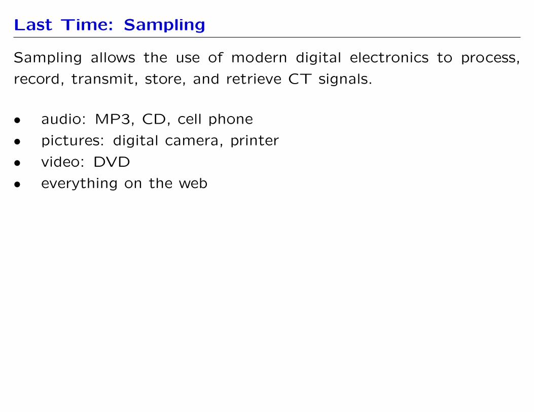
Sampling allows the use of modern digital electronics to process,
record, transmit, store, and retrieve CT signals.
• audio: MP3, CD, cell phone
• pictures: digital camera, printer
• video: DVD
• everything on the web
Last Time: Sampling
ω T
x[n] xr(t)Impulse xp(t) =
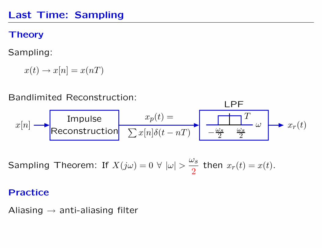
Theory
Sampling:
x(t)→ x[n] = x(nT )
Bandlimited Reconstruction: LPF
Reconstruction � x[n]δ(t − nT ) −ω2s ω
2s
Sampling Theorem: If X(jω) = 0 ∀ |ω| > ω2 s then xr(t) = x(t).
Practice
Aliasing → anti-aliasing filter
Today
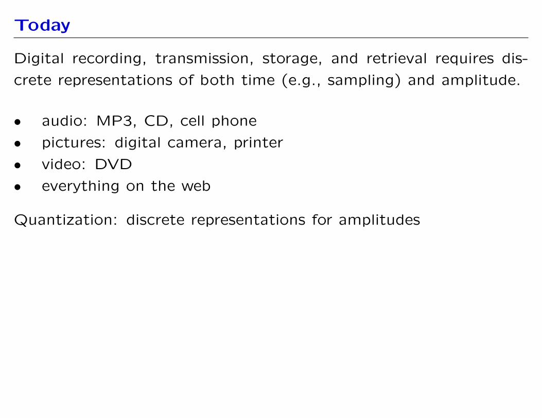
Digital recording, transmission, storage, and retrieval requires dis
crete representations of both time (e.g., sampling) and amplitude.
• audio: MP3, CD, cell phone
• pictures: digital camera, printer
• video: DVD
• everything on the web
Quantization: discrete representations for amplitudes
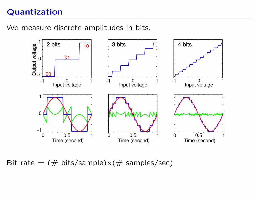
Quantization
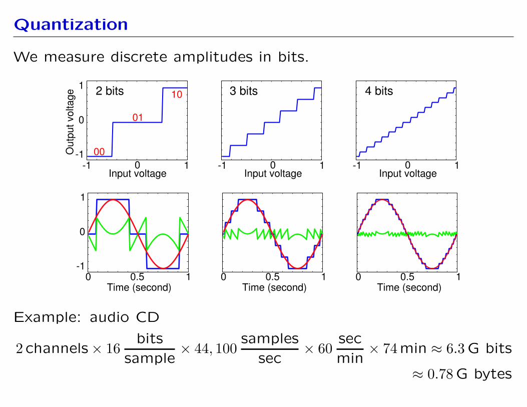
We measure discrete amplitudes in bits.
1
Out
put v
olta
ge
-1 -1
0
0 1
2 bits
00
01
10
-1 0 1 Input voltage Input voltage
3 bits
-1 0 1 Input voltage
4 bits
0 0.5 1 -1
0
1
0 0.5 1 0 0.5 1 Time (second) Time (second) Time (second)
Bit rate = (# bits/sample)×(# samples/sec)
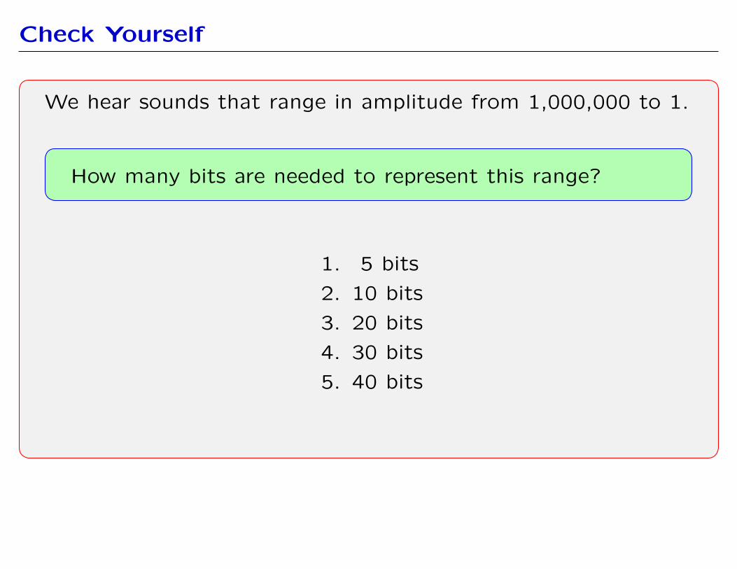
Check Yourself
We hear sounds that range in amplitude from 1,000,000 to 1.
How many bits are needed to represent this range?
1. 5 bits
2. 10 bits
3. 20 bits
4. 30 bits
5. 40 bits
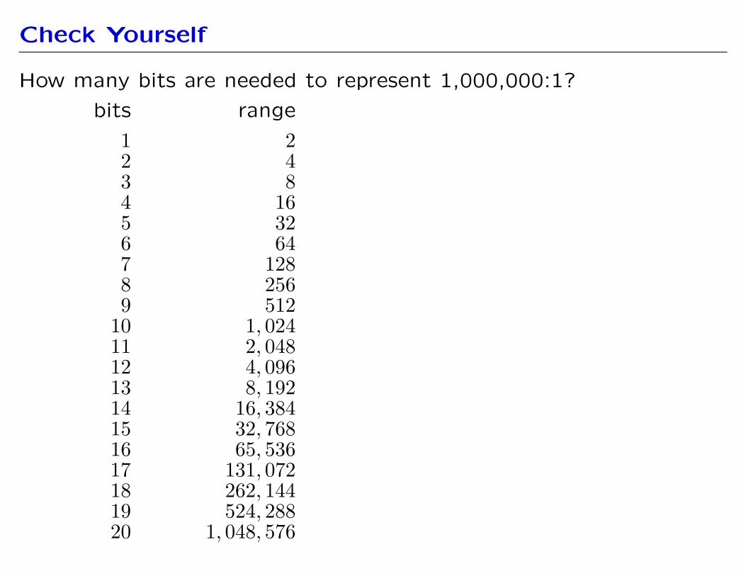
Check Yourself
How many bits are needed to represent 1,000,000:1?
bits range
1 2 2 4 3 8 4 16 5 32 6 64 7 128 8 256 9 512
10 1, 024 11 2, 048 12 4, 096 13 8, 192 14 16, 384 15 32, 768 16 65, 536 17 131, 072 18 262, 144 19 524, 288 20 1, 048, 576
Check Yourself
We hear sounds that range in amplitude from 1,000,000 to 1.
How many bits are needed to represent this range? 3
1. 5 bits
2. 10 bits
3. 20 bits
4. 30 bits
5. 40 bits
Quantization Demonstration
Quantizing Music
• 16 bits/sample
• 8 bits/sample
• 6 bits/sample
• 4 bits/sample
• 3 bits/sample
• 2 bit/sample
J.S. Bach, Sonata No. 1 in G minor Mvmt. IV. Presto
Nathan Milstein, violin
Quantization
We measure discrete amplitudes in bits.
-1
0
1
Out
put v
olta
ge 2 bits 3 bits 4 bits
00
01
10
-1 0 1 -1 0 1 -1 0 1 Input voltage Input voltage Input voltage
-1
0
1
0 0.5 1 0 0.5 1 0 0.5 1 Time (second) Time (second) Time (second)
Example: audio CD
2 channels × 16 bits × 44, 100
samples × 60 sec × 74 min ≈ 6.3 G bits
sample sec min ≈ 0.78 G bytes
Quantizing Images
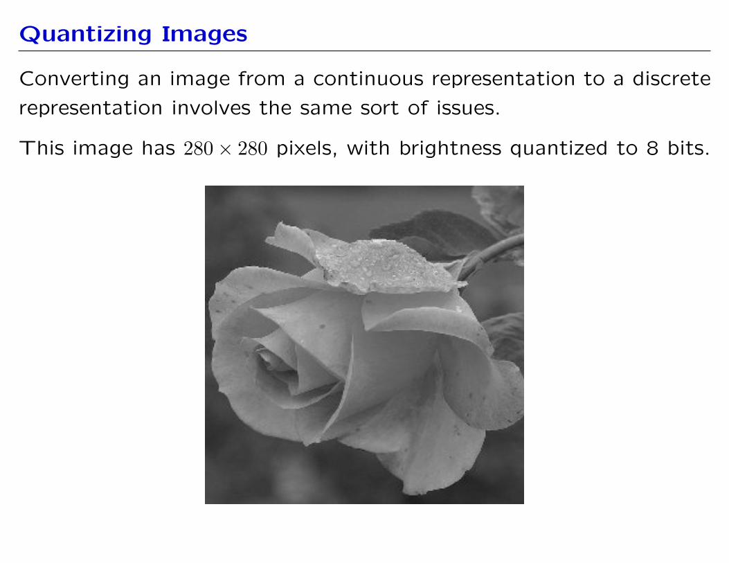
Converting an image from a continuous representation to a discrete
representation involves the same sort of issues.
This image has 280 × 280 pixels, with brightness quantized to 8 bits.
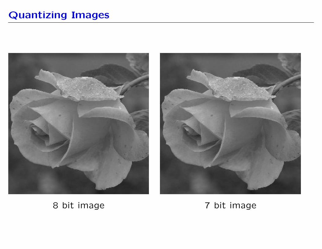
Quantizing Images
8 bit image 7 bit image

Quantizing Images
8 bit image 6 bit image

Quantizing Images
8 bit image 5 bit image
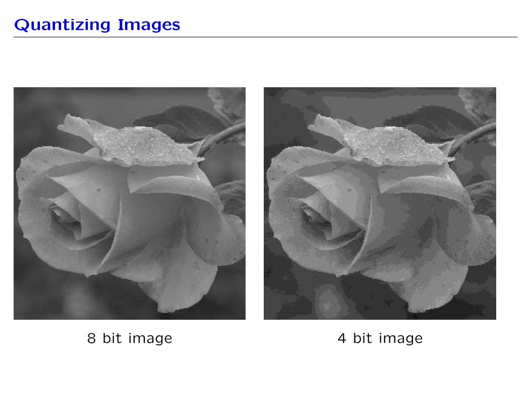
Quantizing Images
8 bit image 4 bit image

Quantizing Images
8 bit image 3 bit image
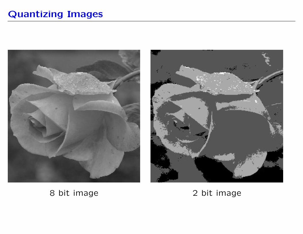
Quantizing Images
8 bit image 2 bit image
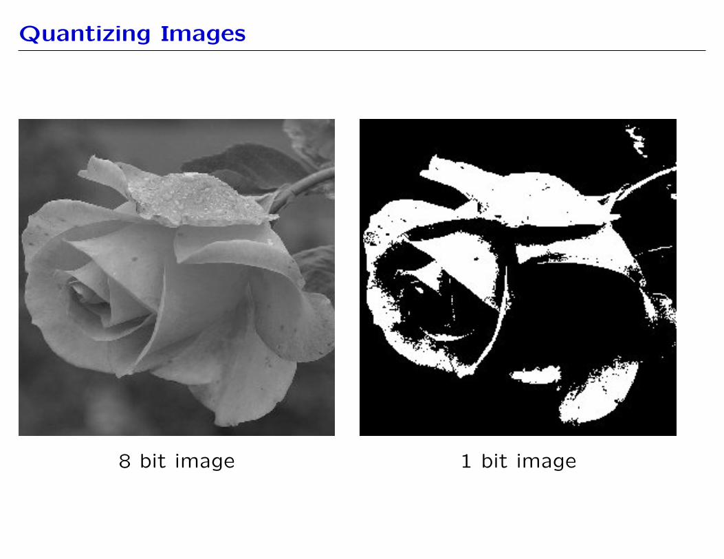
Quantizing Images
8 bit image 1 bit image
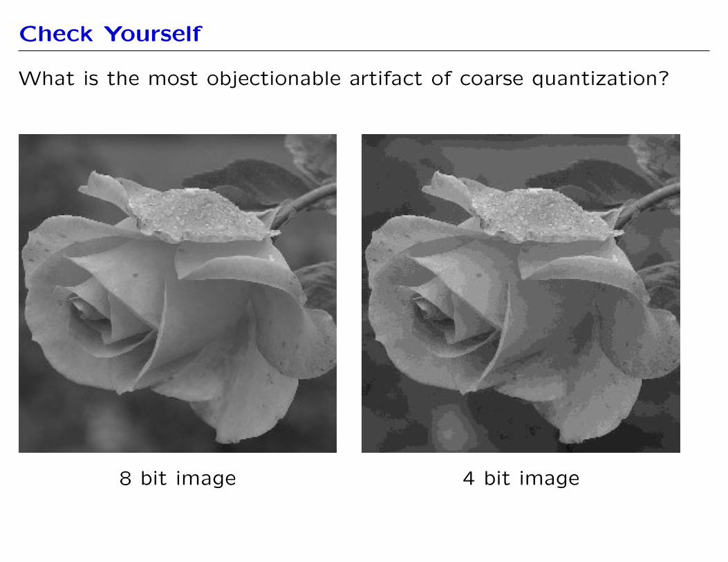
Check Yourself
What is the most objectionable artifact of coarse quantization?
8 bit image 4 bit image
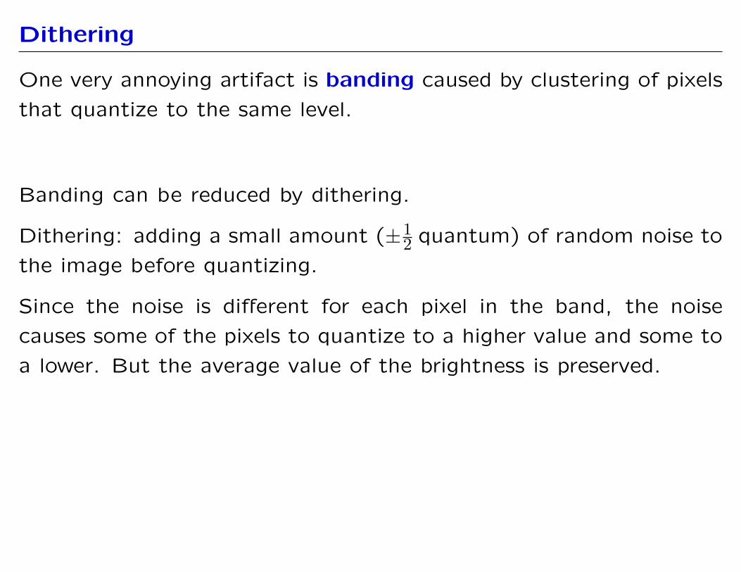
Dithering
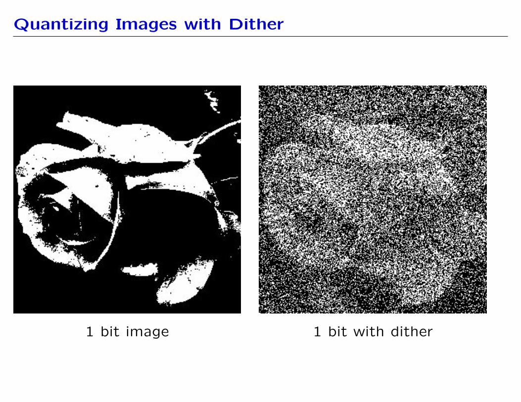
One very annoying artifact is banding caused by clustering of pixels
that quantize to the same level.
Banding can be reduced by dithering.
Dithering: adding a small amount (±12 quantum) of random noise to
the image before quantizing.
Since the noise is different for each pixel in the band, the noise
causes some of the pixels to quantize to a higher value and some to
a lower. But the average value of the brightness is preserved.

Quantizing Images with Dither
7 bit image 7 bits with dither
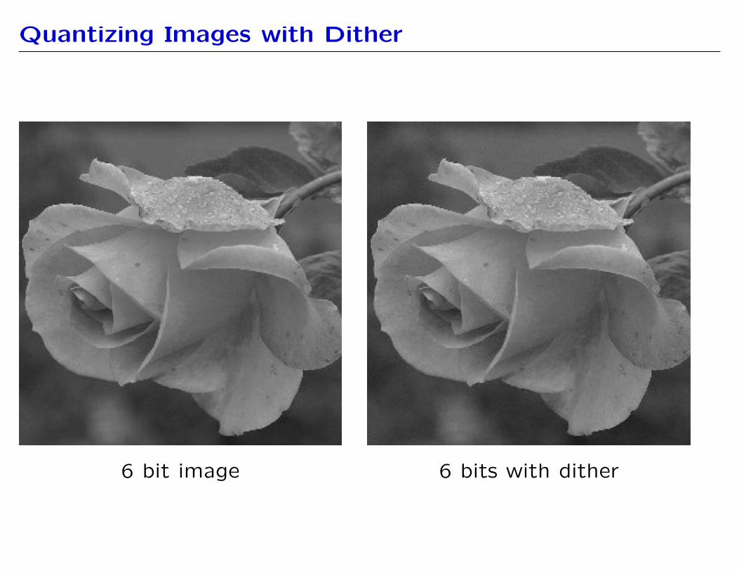
Quantizing Images with Dither
6 bit image 6 bits with dither

Quantizing Images with Dither
5 bit image 5 bits with dither

Quantizing Images with Dither
4 bit image 4 bits with dither

Quantizing Images with Dither
3 bit image 3 bits with dither
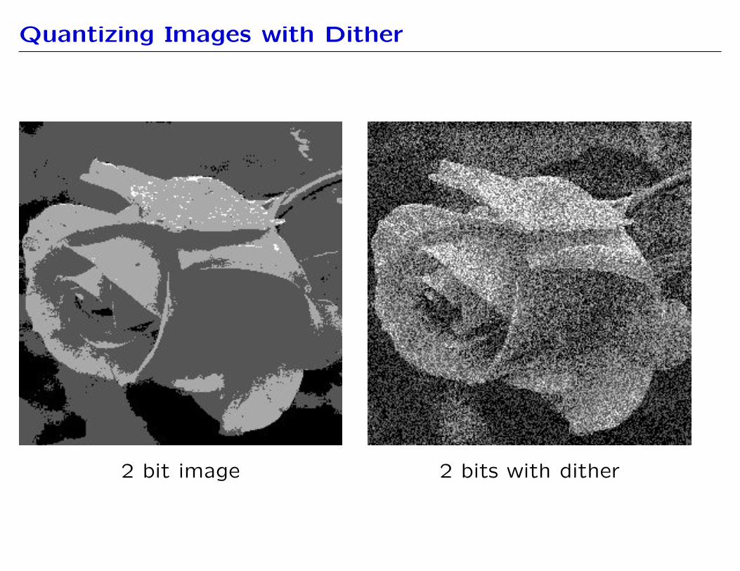
Quantizing Images with Dither
2 bit image 2 bits with dither
Quantizing Images with Dither
1 bit image 1 bit with dither
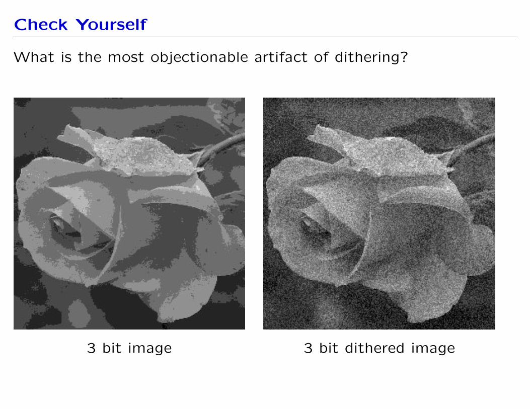
Check Yourself
What is the most objectionable artifact of dithering?
3 bit image 3 bit dithered image
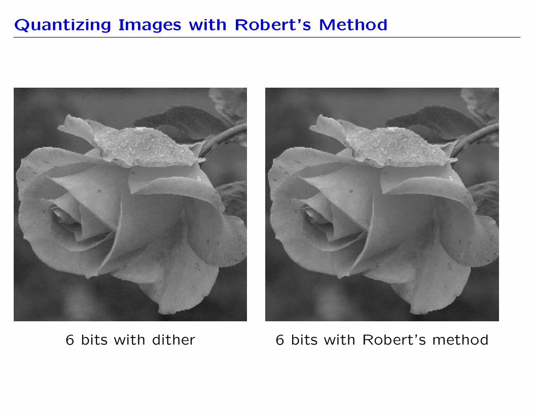
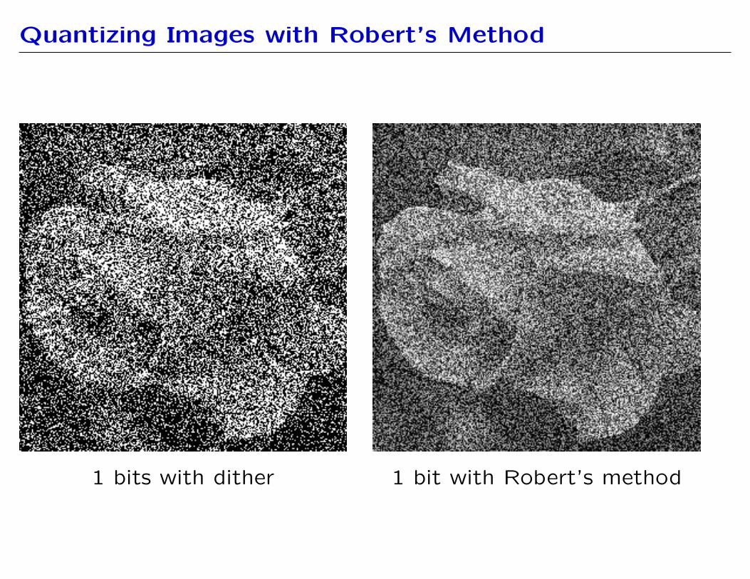
Robert’s Technique
One annoying feature of dithering is that it adds noise.
The noise can be reduced using Robert’s technique.
Robert’s technique: add a small amount (±12 quantum) of random
noise before quantizing, then subtract that same amount of random
noise.
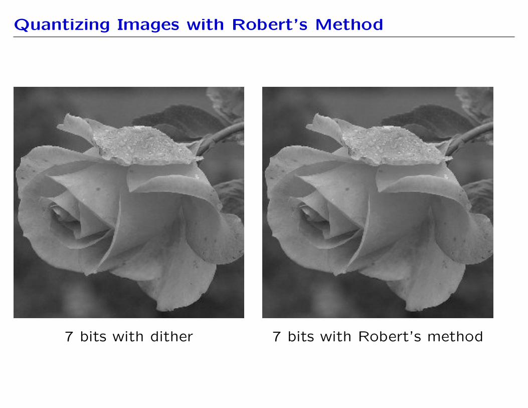
Quantizing Images with Robert’s Method
7 bits with dither 7 bits with Robert’s method
Quantizing Images with Robert’s Method
6 bits with dither 6 bits with Robert’s method
Quantizing Images with Robert’s Method
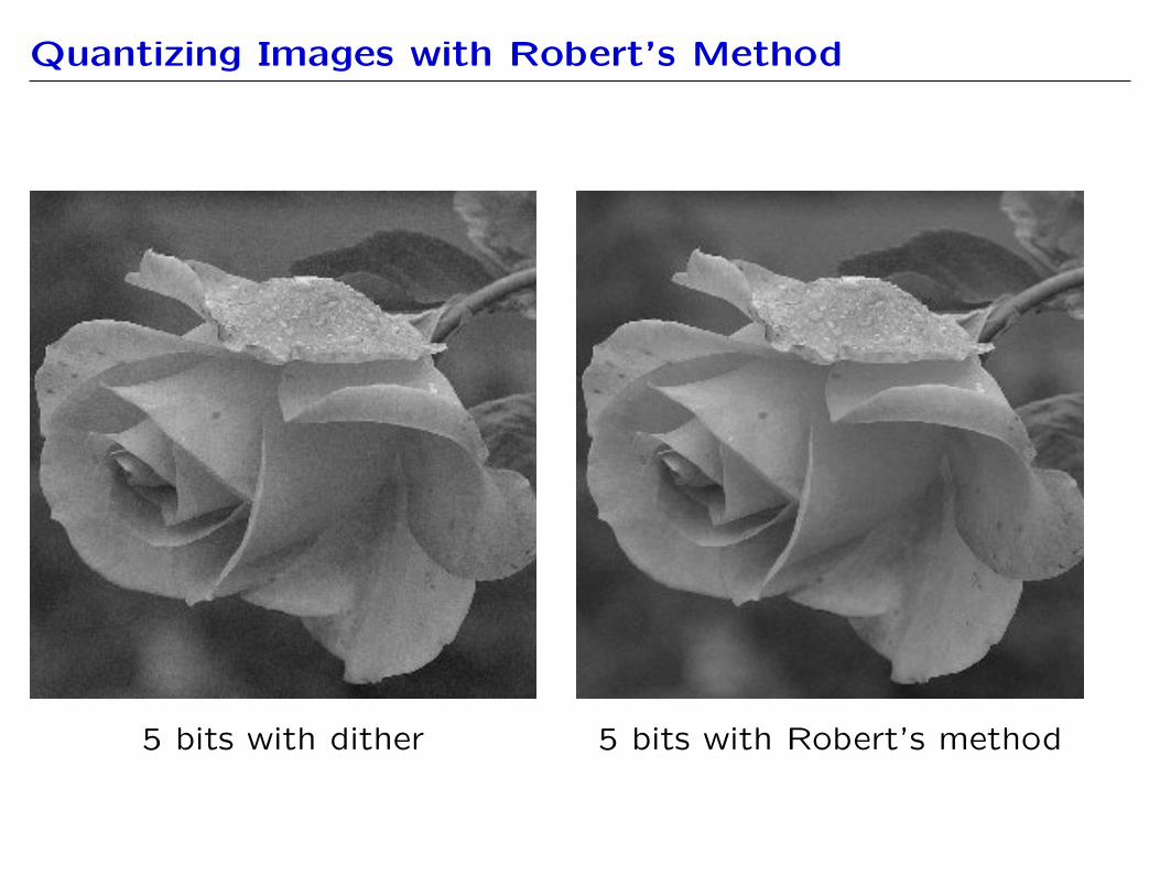
5 bits with dither 5 bits with Robert’s method
Quantizing Images with Robert’s Method
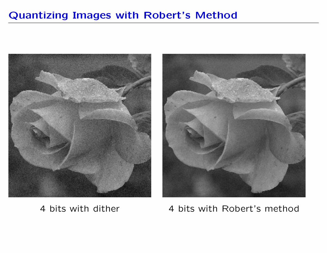
4 bits with dither 4 bits with Robert’s method

Quantizing Images with Robert’s Method
3 bits with dither 3 bits with Robert’s method
Quantizing Images with Robert’s Method
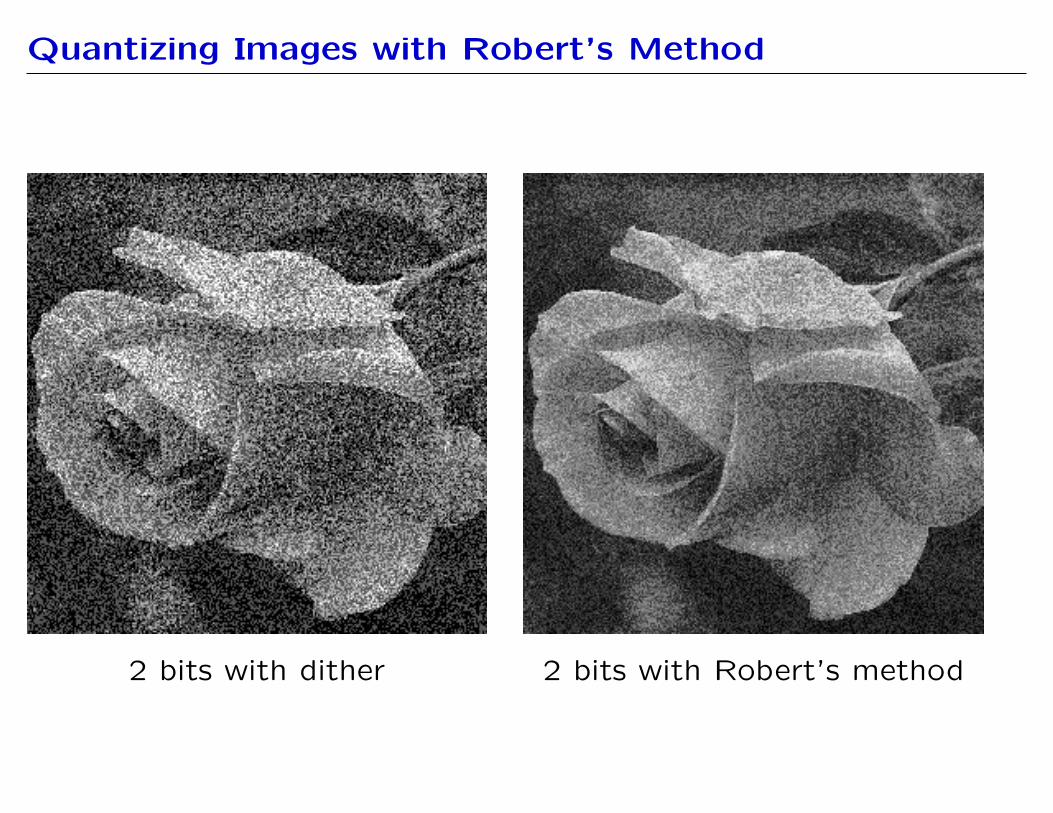
2 bits with dither 2 bits with Robert’s method
Quantizing Images with Robert’s Method
1 bits with dither 1 bit with Robert’s method
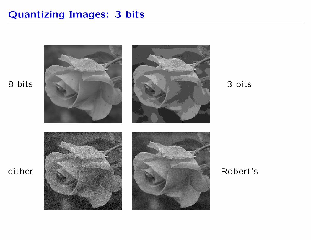
Quantizing Images: 3 bits
8 bits 3 bits
dither Robert’s
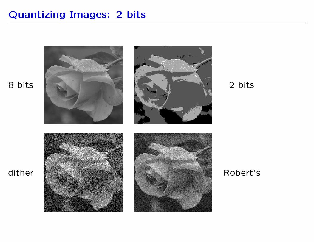
Quantizing Images: 2 bits
8 bits 2 bits
dither Robert’s
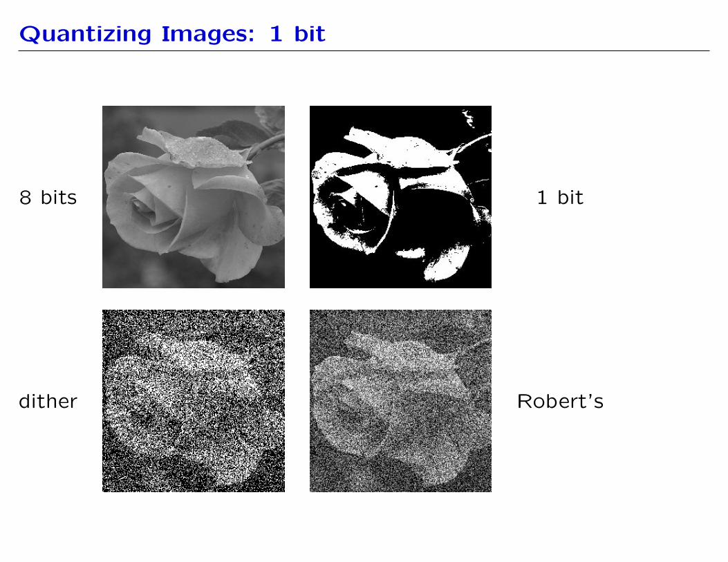
Quantizing Images: 1 bit
8 bits 1 bit
dither Robert’s
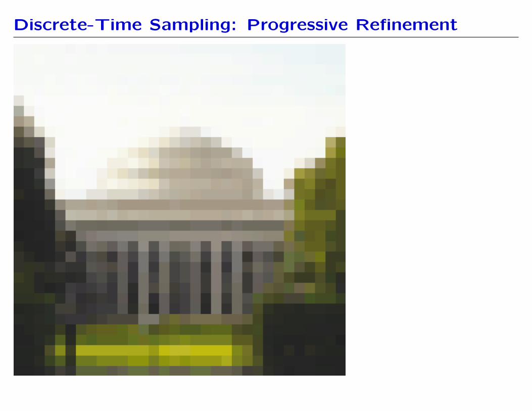
Progressive Refinement
Trading precision for speed.
Start by sending a crude representation, then progressively update
with increasing higher fidelity versions.
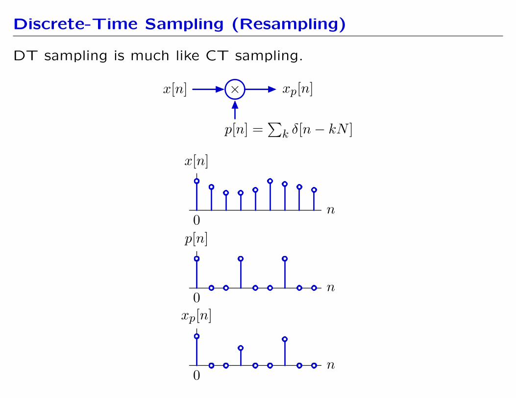
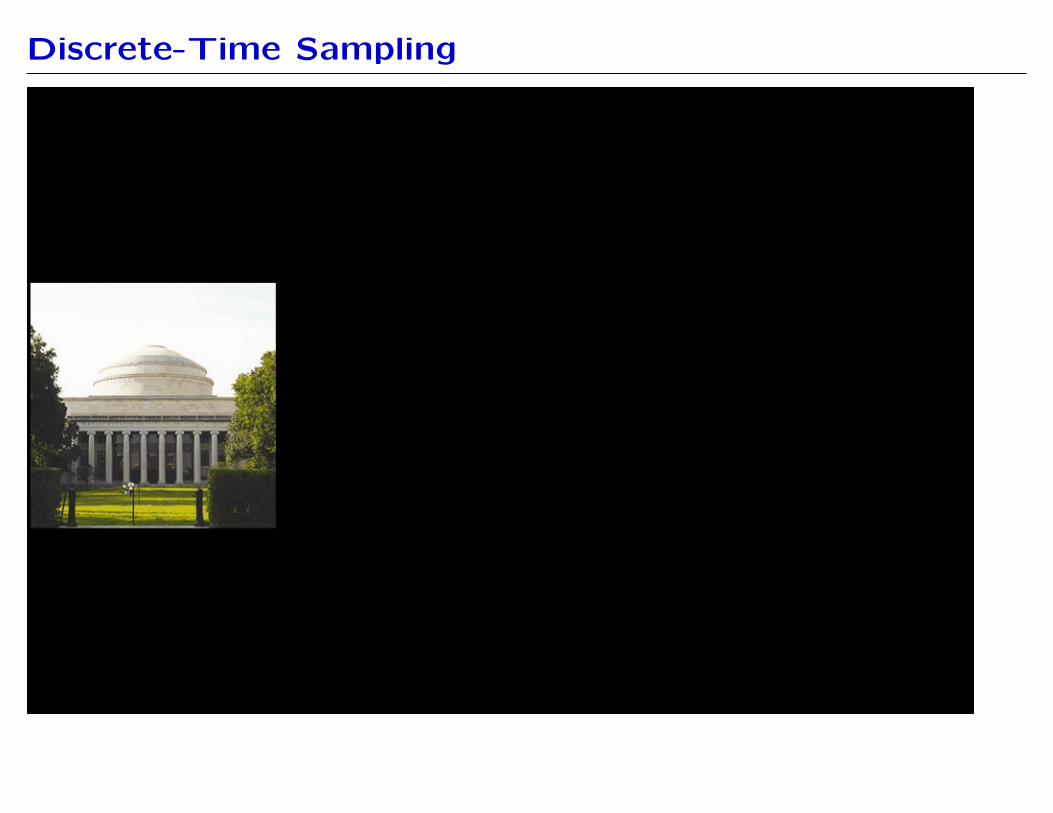
Discrete-Time Sampling (Resampling)
DT sampling is much like CT sampling.
× xp[n]x[n]
p[n] =� k δ[n − kN ]
x[n]
n0
n
p[n]
0xp[n]
n0
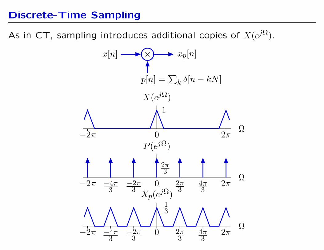
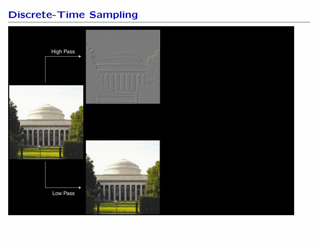
Discrete-Time Sampling
As in CT, sampling introduces additional copies of X(ejΩ).
xp[n]×x[n]
p[n] =� k δ[n − kN ]
X(ejΩ)
0 2π−2π
1
Ω
P (ejΩ)
2π 3
Ω −2π −4π −2π 0 2π 4π 2π3 3
Xp(ejΩ) 3 3
1 3
Ω −2π −4π −2π 0 2π 4π 2π3 3 3 3

� � �
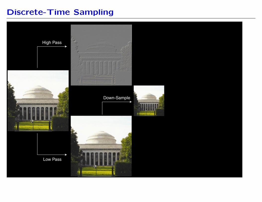
Discrete-Time Sampling
Sampling a finite sequence gives rise to a shorter sequence.
x[n]
0xp[n]
0xb[n]
0
n
n
n
Xb(ejΩ) = xb[n]e −jΩn = xp[3n]e −jΩn = xp[k]e −jΩk/3 = Xp(ejΩ/3) n n k
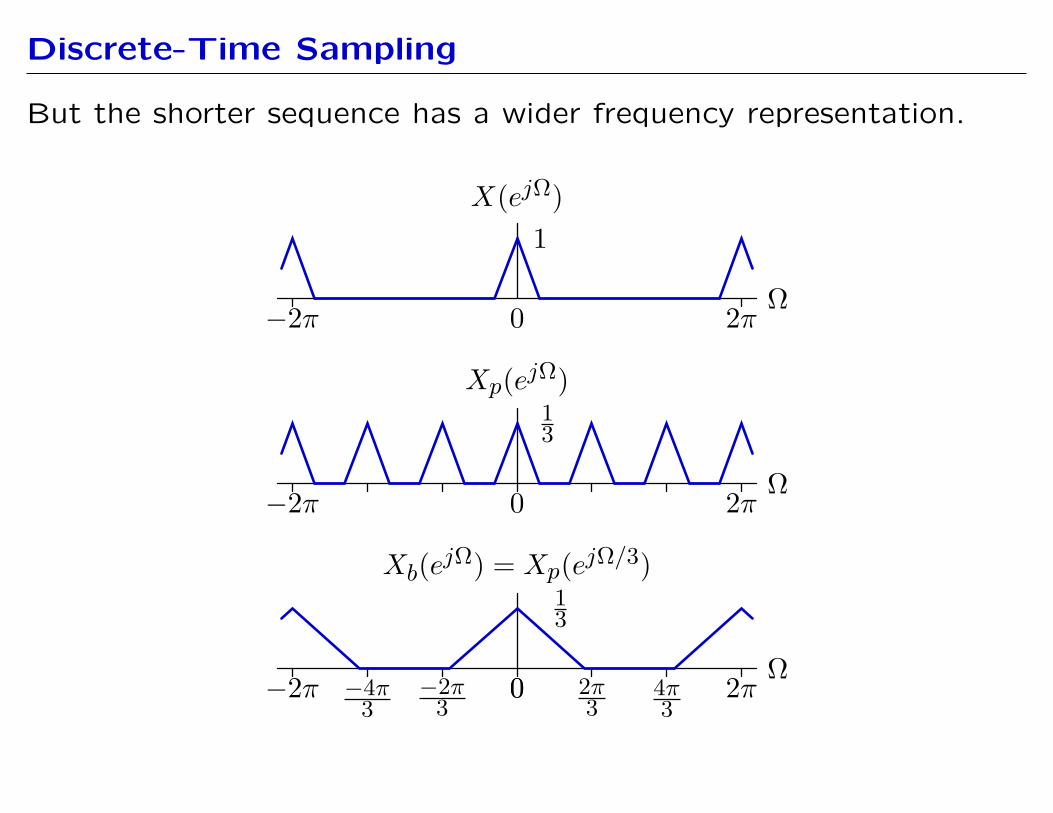
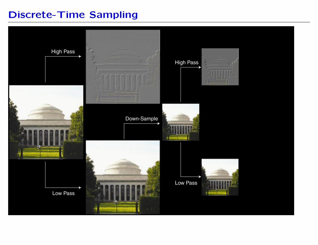
Discrete-Time Sampling
But the shorter sequence has a wider frequency representation.
X(ejΩ)
2π−2π
1
Ω0
Xp(ejΩ)
0 2π−2π
1 3
Ω
Xb(ejΩ) = Xp(ejΩ/3)1 3
Ω −2π −4π −2π 00 2π 4π 2π3 3 3 3
Discrete-Time Sampling
Discrete-Time Sampling
Discrete-Time Sampling
Discrete-Time Sampling
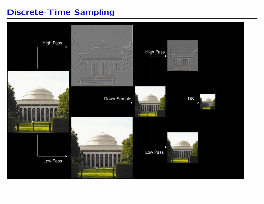
Discrete-Time Sampling

Discrete-Time Sampling
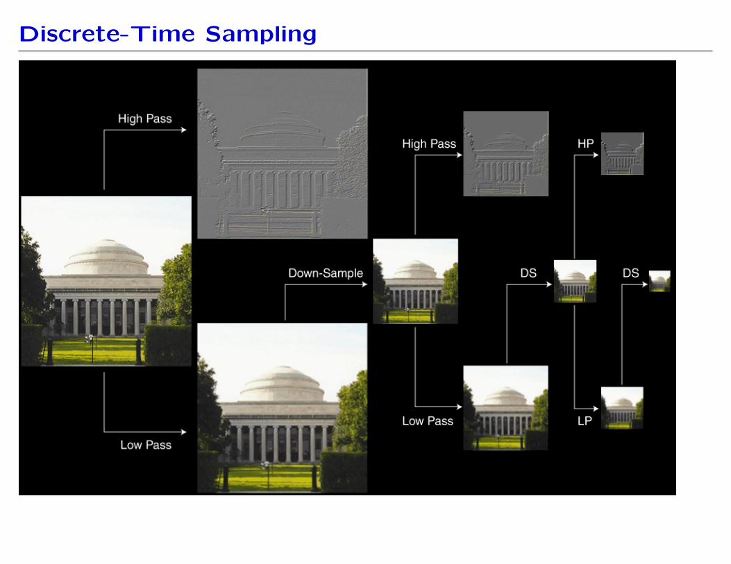
Discrete-Time Sampling
� � �
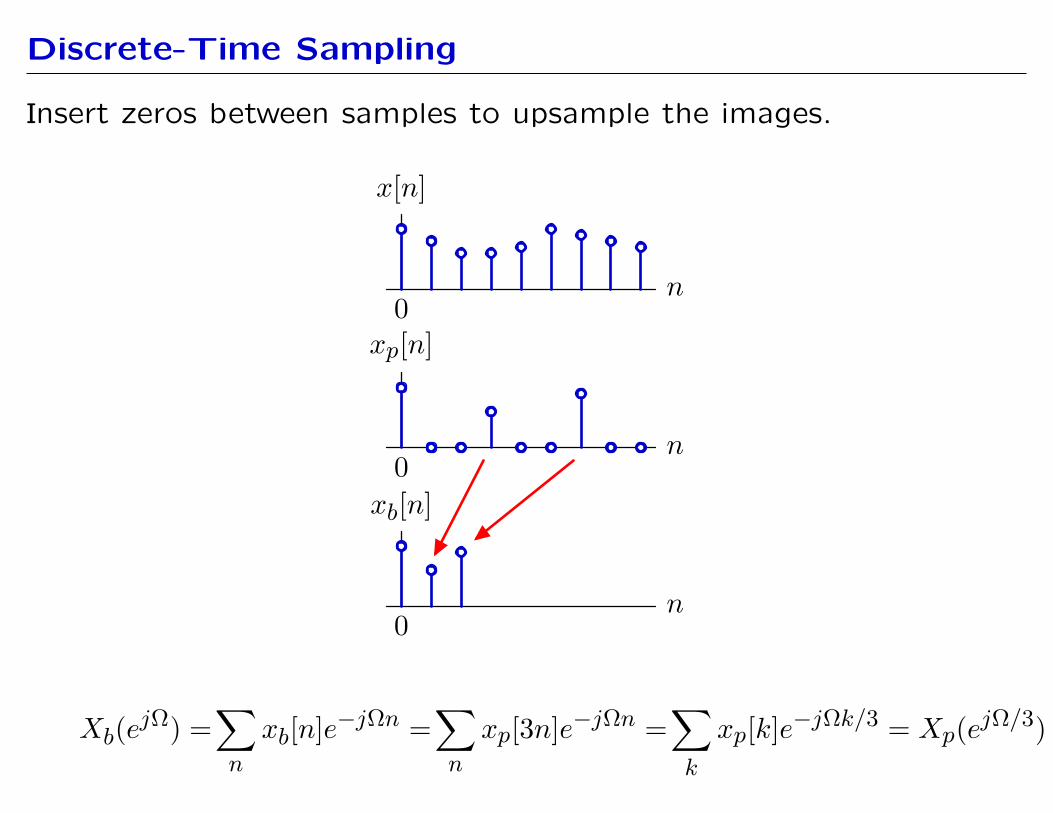
Discrete-Time Sampling
Insert zeros between samples to upsample the images.
x[n]
0xp[n]
0xb[n]
0
n
n
n
Xb(ejΩ) = xb[n]e −jΩn = xp[3n]e −jΩn = xp[k]e −jΩk/3 = Xp(ejΩ/3) n n k
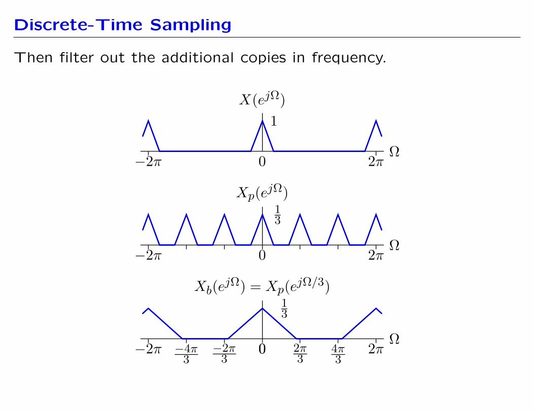
Discrete-Time Sampling
Then filter out the additional copies in frequency.
X(ejΩ)
2π−2π
1
Ω0
Xp(ejΩ)
0 2π−2π
1 3
Ω
Xb(ejΩ) = Xp(ejΩ/3)13
Ω −2π −4π −2π 00 2π 4π 2π3 3 3 3
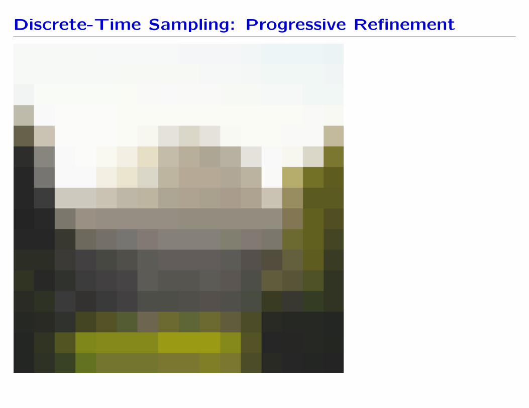
Discrete-Time Sampling: Progressive Refinement
Discrete-Time Sampling: Progressive Refinement

Discrete-Time Sampling: Progressive Refinement

Discrete-Time Sampling: Progressive Refinement

Discrete-Time Sampling: Progressive Refinement
Perceptual Coding
Quantizing in the Fourier domain: JPEG.
JPEG
Example: JPEG (“Joint Photographic Experts Group”) encodes im
ages by a sequence of transformations:
• color encoding
• DCT (discrete cosine transform): a kind of Fourier series
• quantization to achieve perceptual compression (lossy)
• Huffman encoding: lossless information theoretic coding
We will focus on the DCT and quantization of its components.
• the image is broken into 8 × 8 pixel blocks
• each block is represented by its 8 × 8 DCT coefficients
• each DCT coefficient is quantized, using higher resolutions for
coefficients with greater perceptual importance
JPEG
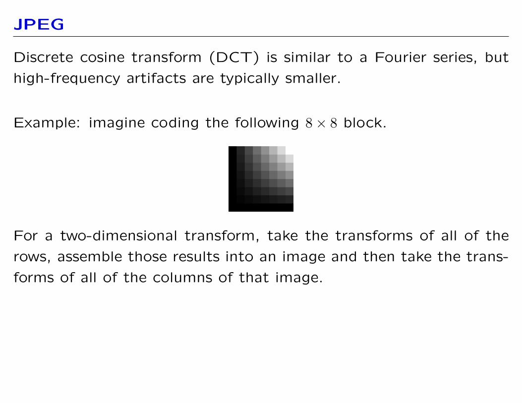
Discrete cosine transform (DCT) is similar to a Fourier series, but
high-frequency artifacts are typically smaller.
Example: imagine coding the following 8 × 8 block.
For a two-dimensional transform, take the transforms of all of the
rows, assemble those results into an image and then take the trans
forms of all of the columns of that image.
�
JPEG
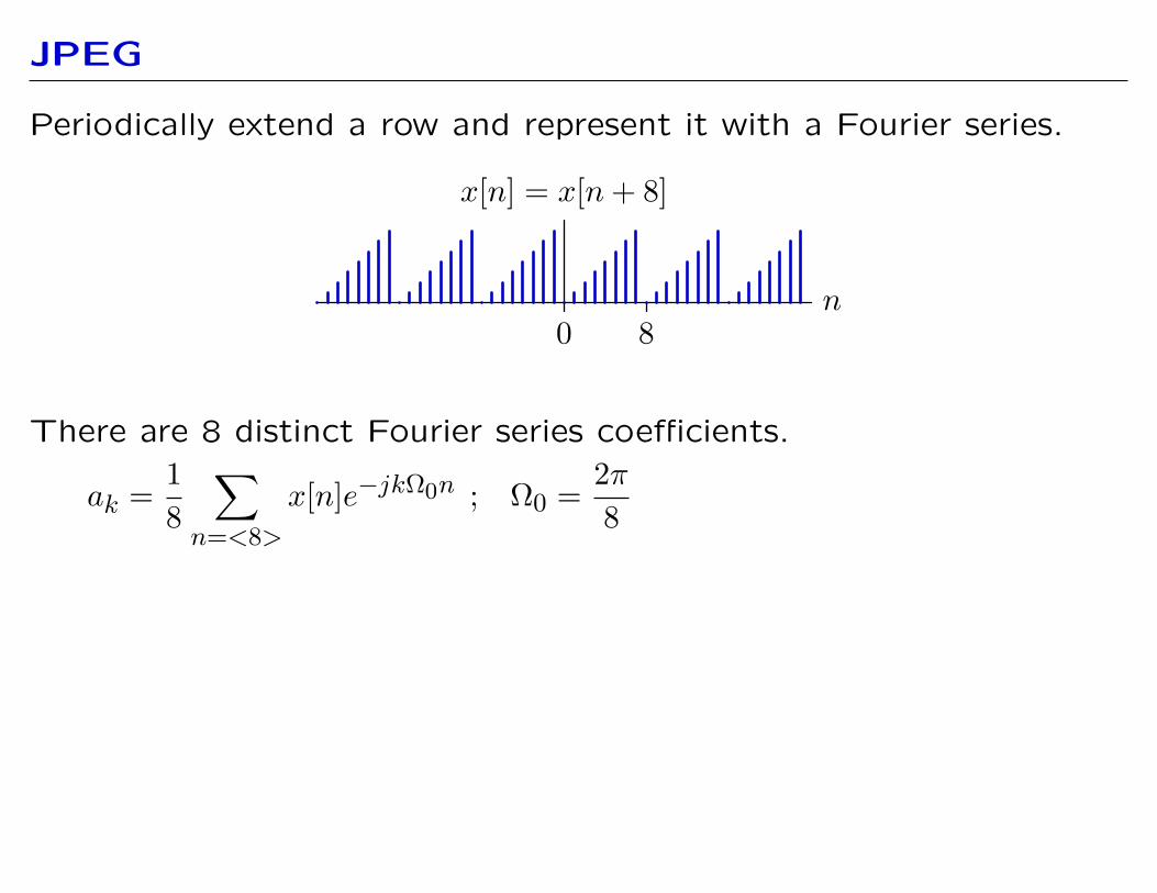
Periodically extend a row and represent it with a Fourier series.
x[n] = x[n + 8]
n0 8
There are 8 distinct Fourier series coefficients.
ak = 81
x[n]e −jkΩ0n ; Ω0 = 28 π
n=<8>
JPEG
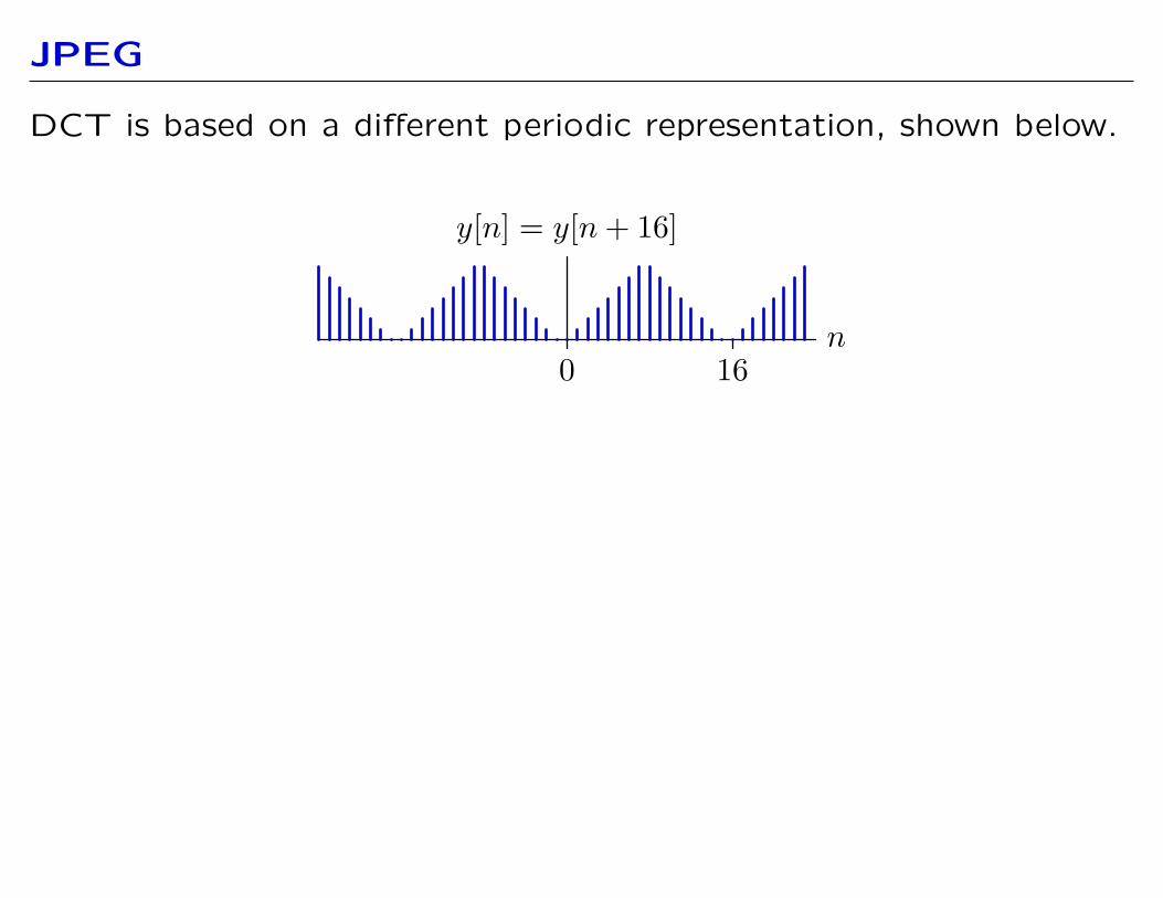
DCT is based on a different periodic representation, shown below.
y[n] = y[n + 16]
n 0 16
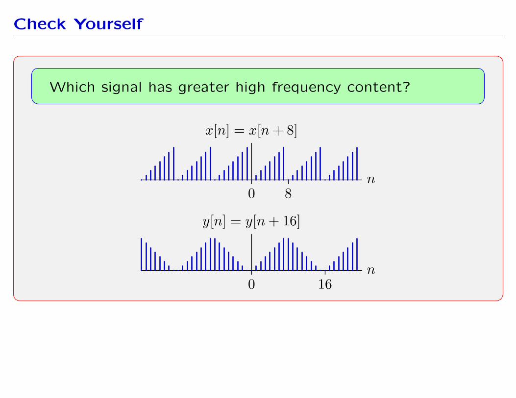
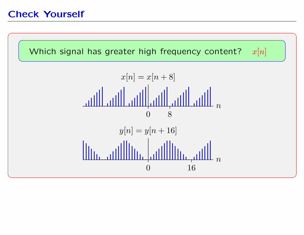
Check Yourself
Which signal has greater high frequency content?
x[n] = x[n + 8]
n 0 8
y[n] = y[n + 16]
n 0 16
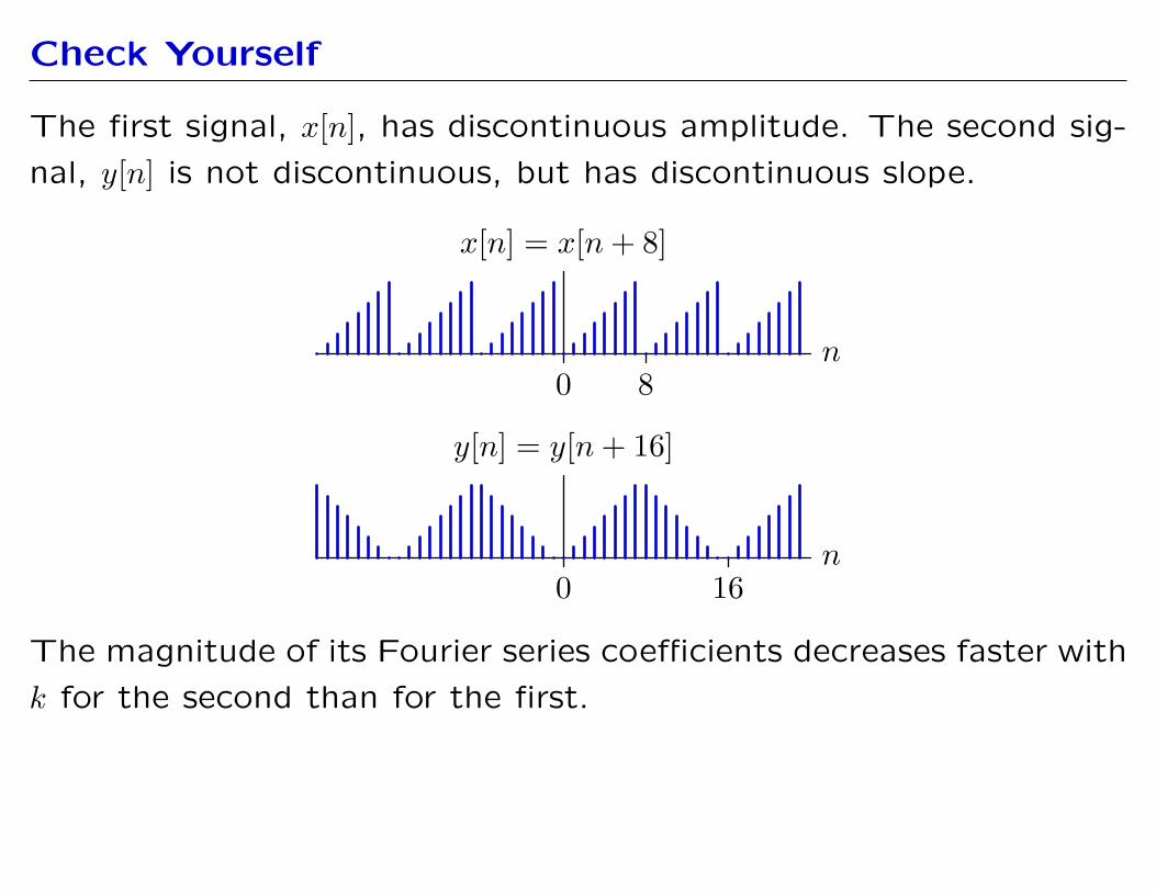
Check Yourself
The first signal, x[n], has discontinuous amplitude. The second sig
nal, y[n] is not discontinuous, but has discontinuous slope.
x[n] = x[n + 8]
n 0 8
y[n] = y[n + 16]
n 0 16
The magnitude of its Fourier series coefficients decreases faster with
k for the second than for the first.
Check Yourself
Which signal has greater high frequency content? x[n]
x[n] = x[n + 8]
n 0 8
y[n] = y[n + 16]
n 0 16
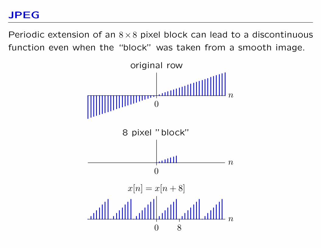
JPEG
Periodic extension of an 8× 8 pixel block can lead to a discontinuous
function even when the “block” was taken from a smooth image.
original row
n 0
8 pixel ”block”
n 0
x[n] = x[n + 8]
n 0 8
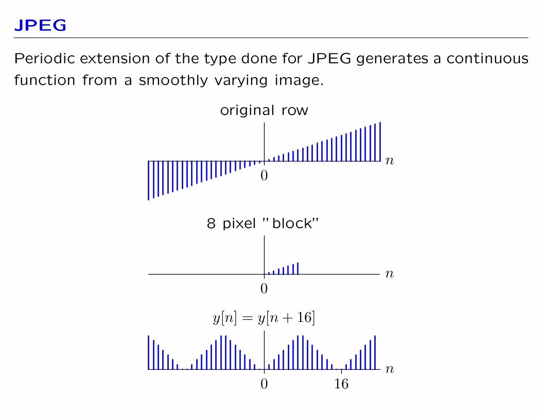
JPEG
Periodic extension of the type done for JPEG generates a continuous
function from a smoothly varying image.
original row
n 0
8 pixel ”block”
n 0
y[n] = y[n + 16]
n 0 16
JPEG
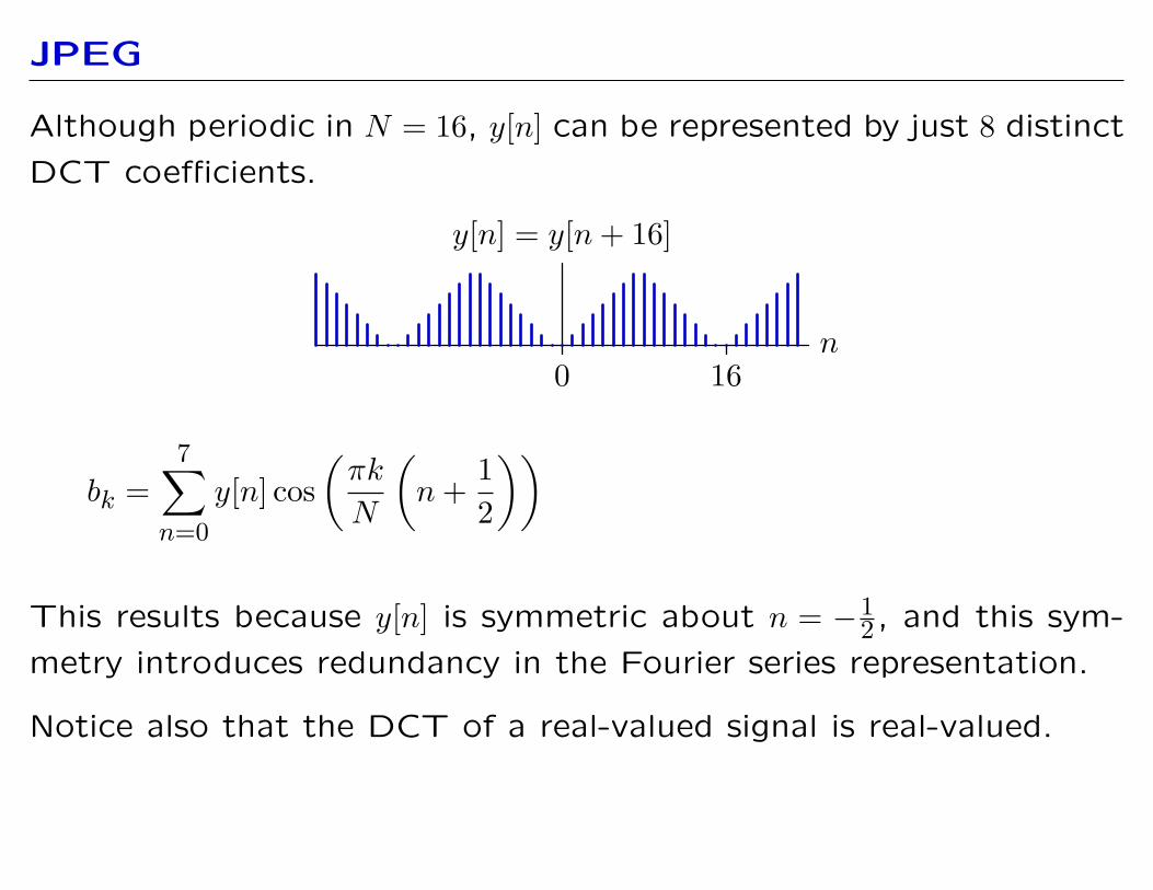
Although periodic in N = 16, y[n] can be represented by just 8 distinct
DCT coefficients.
y[n] = y[n + 16]
n0 16
7 � � �� � πk 1 bk = y[n] cos n +
N 2 n=0
This results because y[n] is symmetric about n = −21 , and this sym
metry introduces redundancy in the Fourier series representation.
Notice also that the DCT of a real-valued signal is real-valued.
JPEG
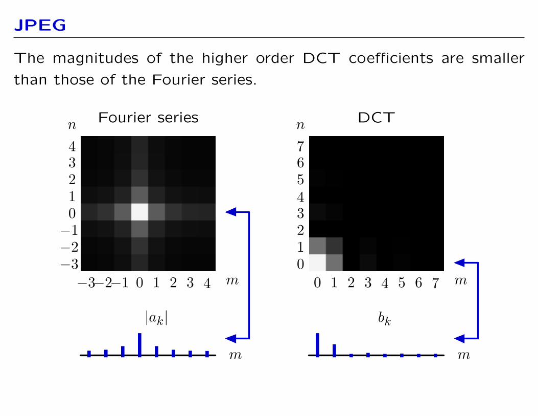
The magnitudes of the higher order DCT coefficients are smaller
than those of the Fourier series.
Fourier seriesn
43210−1−2−3−3−2−1 0 1 2 3 4 m
|ak|
m
DCT n
76543210
0 1 2 3 4 5 6 7 m
bk
m
JPEG
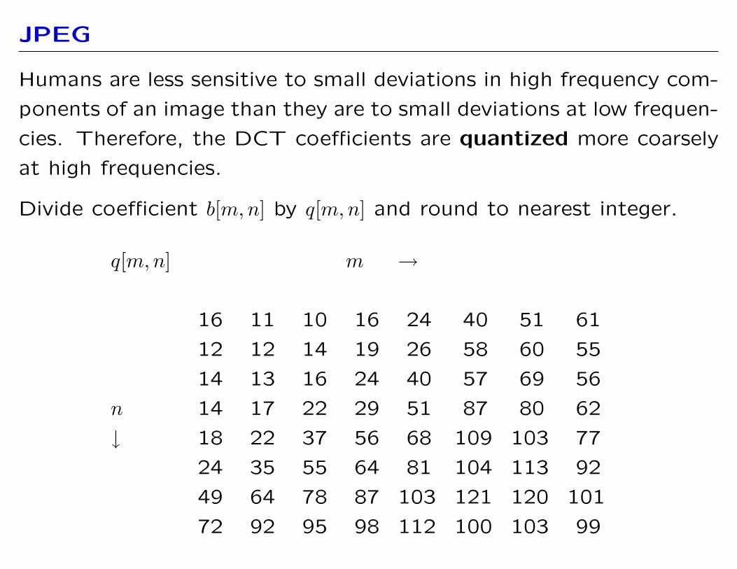
Humans are less sensitive to small deviations in high frequency com
ponents of an image than they are to small deviations at low frequen
cies. Therefore, the DCT coefficients are quantized more coarsely
at high frequencies.
Divide coefficient b[m,n] by q[m,n] and round to nearest integer.
q[m,n] m →
16 11 10 16 24 40 51 61
12 12 14 19 26 58 60 55
14 13 16 24 40 57 69 56
n 14 17 22 29 51 87 80 62
↓ 18 22 37 56 68 109 103 77
24 35 55 64 81 104 113 92
49 64 78 87 103 121 120 101
72 92 95 98 112 100 103 99
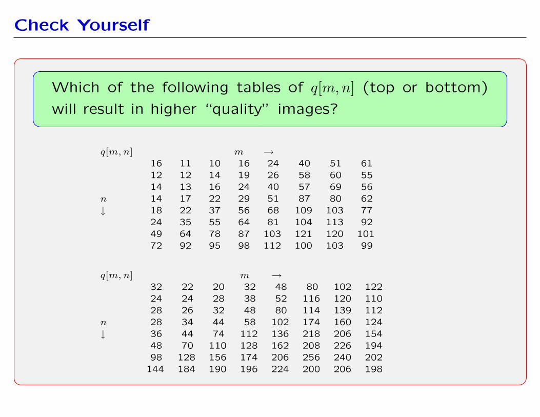
Check Yourself
Which of the following tables of q[m, n] (top or bottom)
will result in higher “quality” images?
q[m, n] m → 16 11 10 16 24 40 51 61 12 12 14 19 26 58 60 55 14 13 16 24 40 57 69 56
n 14 17 22 29 51 87 80 62 ↓ 18 22 37 56 68 109 103 77
24 35 55 64 81 104 113 92 49 64 78 87 103 121 120 101 72 92 95 98 112 100 103 99
q[m, n] m → 32 22 20 32 48 80 102 122 24 24 28 38 52 116 120 110 28 26 32 48 80 114 139 112
n 28 34 44 58 102 174 160 124 ↓ 36 44 74 112 136 218 206 154
48 70 110 128 162 208 226 194 98 128 156 174 206 256 240 202
144 184 190 196 224 200 206 198
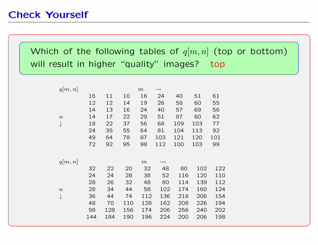
Check Yourself
Which of the following tables of q[m, n] (top or bottom)
will result in higher “quality” images? top
q[m, n] m → 16 11 10 16 24 40 51 61 12 12 14 19 26 58 60 55 14 13 16 24 40 57 69 56
n 14 17 22 29 51 87 80 62 ↓ 18 22 37 56 68 109 103 77
24 35 55 64 81 104 113 92 49 64 78 87 103 121 120 101 72 92 95 98 112 100 103 99
q[m, n] m → 32 22 20 32 48 80 102 122 24 24 28 38 52 116 120 110 28 26 32 48 80 114 139 112
n 28 34 44 58 102 174 160 124 ↓ 36 44 74 112 136 218 206 154
48 70 110 128 162 208 226 194 98 128 156 174 206 256 240 202
144 184 190 196 224 200 206 198
JPEG
Finally, encode the DCT coefficients for each block using “run
length” encoding followed by an information theoretic (lossless)
“Huffman” scheme, in which frequently occuring patterns are
represented by short codes.
The “quality” of the image can be adjusted by changing the values
of q[m,n]. Large values of q[m,n] result in large “runs” of zeros,
which compress well.
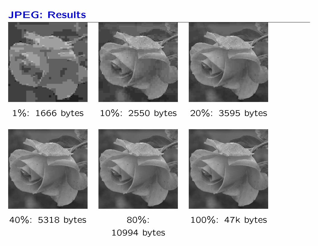
JPEG: Results
1%: 1666 bytes 10%: 2550 bytes 20%: 3595 bytes
40%: 5318 bytes 80%: 100%: 47k bytes
10994 bytes
MIT OpenCourseWarehttp://ocw.mit.edu
6.003 Signals and Systems Spring 2010
For information about citing these materials or our Terms of Use, visit: http://ocw.mit.edu/terms.