§5.5: Ekman Pumping

Effective Depth of Ekman Layer.

2

Effective Depth of Ekman Layer.Defining γ =

√f/2K, we derived the solution

u = ug(1− e−γz cos γz)

v = uge−γz sin γz

corresponding to the Ekman spiral.

2

Effective Depth of Ekman Layer.Defining γ =

√f/2K, we derived the solution

u = ug(1− e−γz cos γz)

v = uge−γz sin γz

corresponding to the Ekman spiral.

Let us assume the values f = 10−4 s−1 and K = 5m2s−1.

2

Effective Depth of Ekman Layer.Defining γ =

√f/2K, we derived the solution

u = ug(1− e−γz cos γz)

v = uge−γz sin γz

corresponding to the Ekman spiral.

Let us assume the values f = 10−4 s−1 and K = 5m2s−1.

The effective depth is D = π/γ.

2

Effective Depth of Ekman Layer.Defining γ =

√f/2K, we derived the solution

u = ug(1− e−γz cos γz)

v = uge−γz sin γz

corresponding to the Ekman spiral.

Let us assume the values f = 10−4 s−1 and K = 5m2s−1.

The effective depth is D = π/γ.

With f = 10−4 s−1 and K = 5m2s−1 we have

D =π

γ= π

√2K

f= π

√2× 5

10−4= 993 m ≈ 1 km

Thus, the effective depth of the Ekman boundary layeris about one kilometre.

2

Effective Depth of Ekman Layer.Defining γ =

√f/2K, we derived the solution

u = ug(1− e−γz cos γz)

v = uge−γz sin γz

corresponding to the Ekman spiral.

Let us assume the values f = 10−4 s−1 and K = 5m2s−1.

The effective depth is D = π/γ.

With f = 10−4 s−1 and K = 5m2s−1 we have

D =π

γ= π

√2K

f= π

√2× 5

10−4= 993 m ≈ 1 km

Thus, the effective depth of the Ekman boundary layeris about one kilometre.

Note that D depends on the values of f and K so the par-ticular value 1 km is more an indication of the scale that asharp quantitative estimate.

2

Remarks on the Ekman Spiral

3

Remarks on the Ekman Spiral• The Ekman theory predicts a cross-isobar flow of 45◦ at

the lower boundary. This is not in agreement with obser-vations

3

Remarks on the Ekman Spiral• The Ekman theory predicts a cross-isobar flow of 45◦ at

the lower boundary. This is not in agreement with obser-vations

• Better agreement can be obtained by coupling the Ek-man layer to a surface layer where the wind direction isunchanging and the speed varies logarithmically

3

Remarks on the Ekman Spiral• The Ekman theory predicts a cross-isobar flow of 45◦ at

the lower boundary. This is not in agreement with obser-vations

• Better agreement can be obtained by coupling the Ek-man layer to a surface layer where the wind direction isunchanging and the speed varies logarithmically

• This can be done by taking a boundary condition

V ‖ ∂V

∂z@ z = zB

3

Remarks on the Ekman Spiral• The Ekman theory predicts a cross-isobar flow of 45◦ at

the lower boundary. This is not in agreement with obser-vations

• Better agreement can be obtained by coupling the Ek-man layer to a surface layer where the wind direction isunchanging and the speed varies logarithmically

• This can be done by taking a boundary condition

V ‖ ∂V

∂z@ z = zB

• The solution is then called a modified Ekman spiral.

3

Remarks on the Ekman Spiral• The Ekman theory predicts a cross-isobar flow of 45◦ at

the lower boundary. This is not in agreement with obser-vations

• Better agreement can be obtained by coupling the Ek-man layer to a surface layer where the wind direction isunchanging and the speed varies logarithmically

• This can be done by taking a boundary condition

V ‖ ∂V

∂z@ z = zB

• The solution is then called a modified Ekman spiral.

The modified Ekman Layer is discussed on Holton (§5.3.6).We will not discuss it here.

3

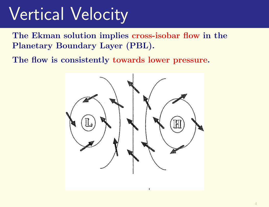
Vertical VelocityThe Ekman solution implies cross-isobar flow in thePlanetary Boundary Layer (PBL).

4

Vertical VelocityThe Ekman solution implies cross-isobar flow in thePlanetary Boundary Layer (PBL).

The flow is consistently towards lower pressure.

4

Vertical VelocityThe Ekman solution implies cross-isobar flow in thePlanetary Boundary Layer (PBL).

The flow is consistently towards lower pressure.

4

For a steady-state solution, the convergence towards lowerpressure centres and divergence from higher pressure cen-tres has two implications:

5

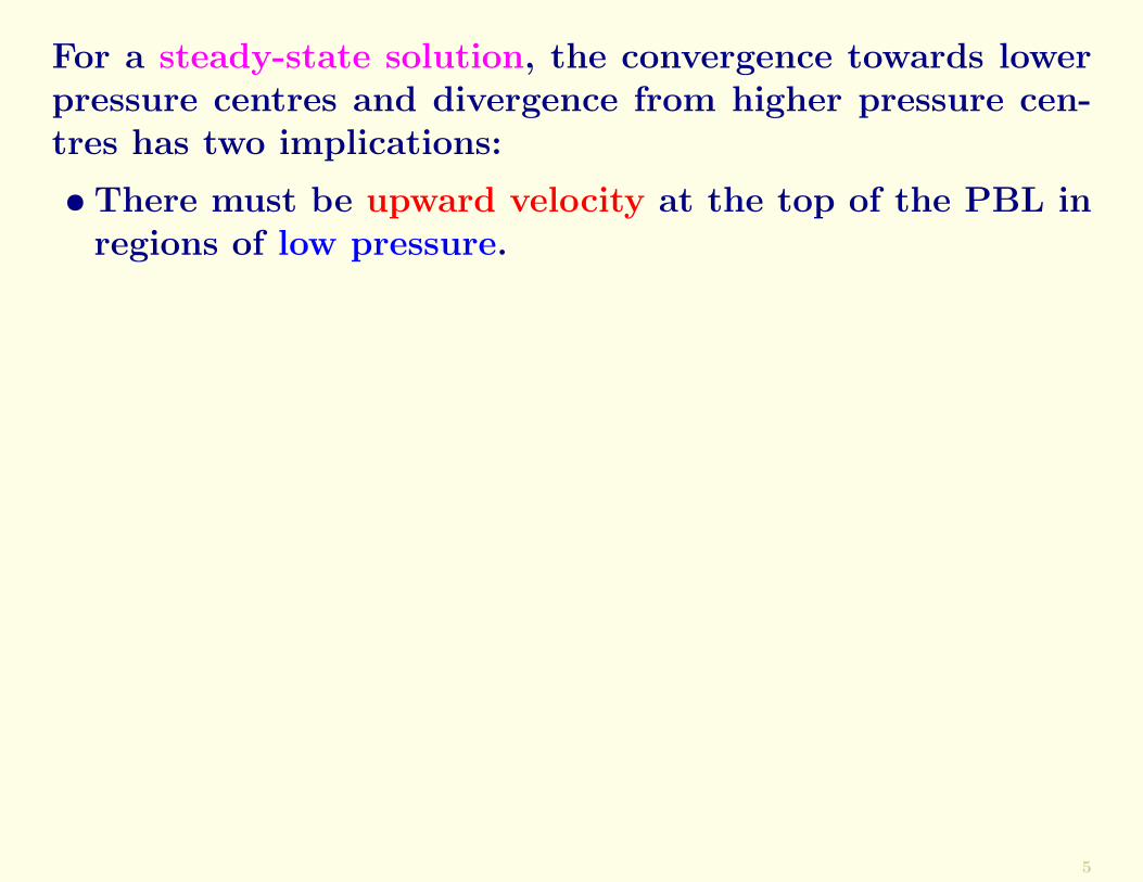
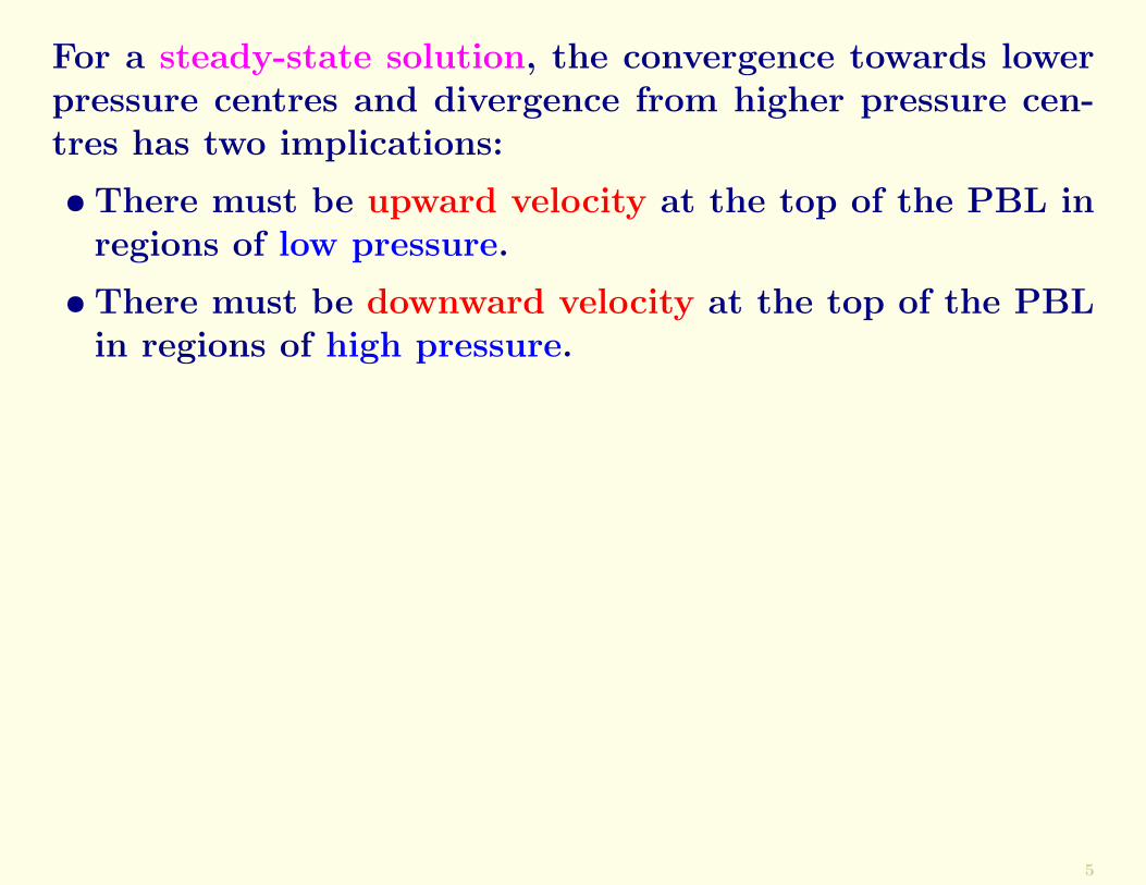
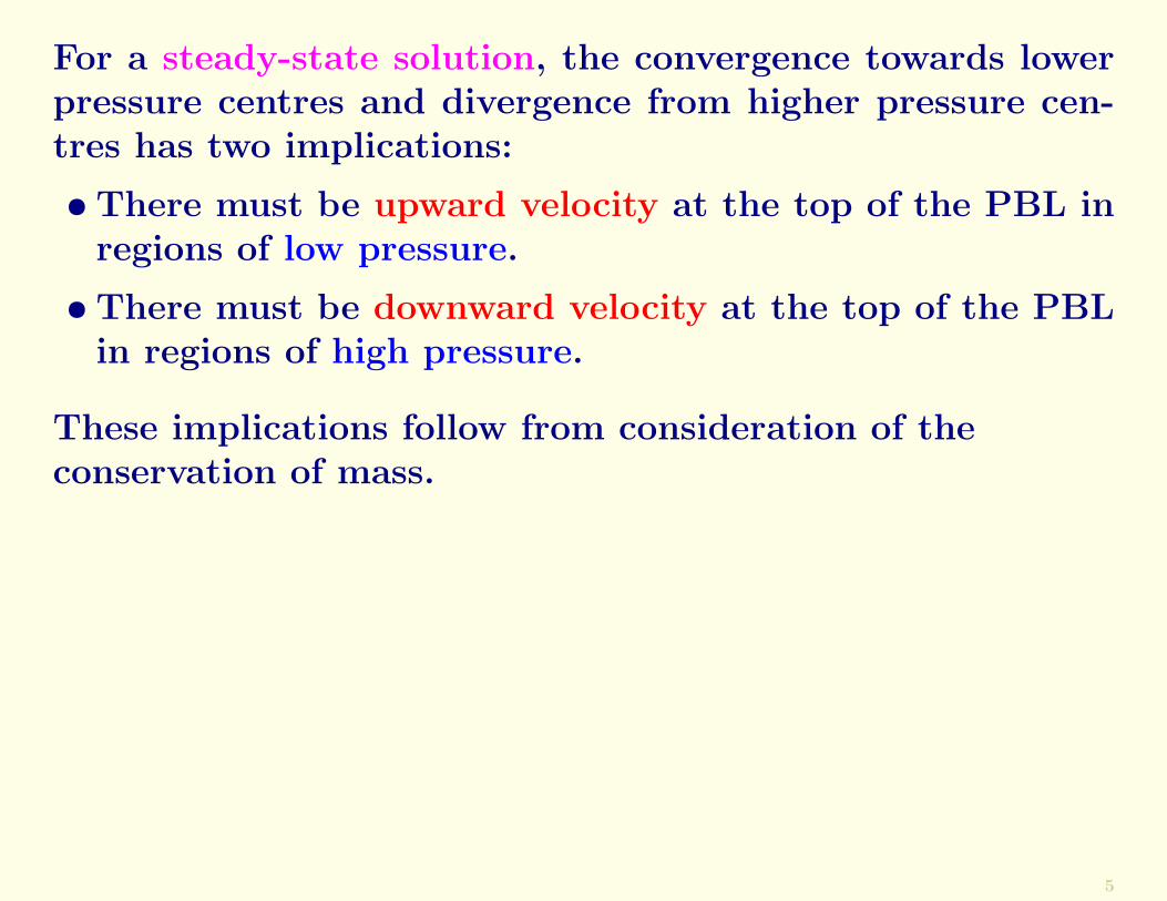
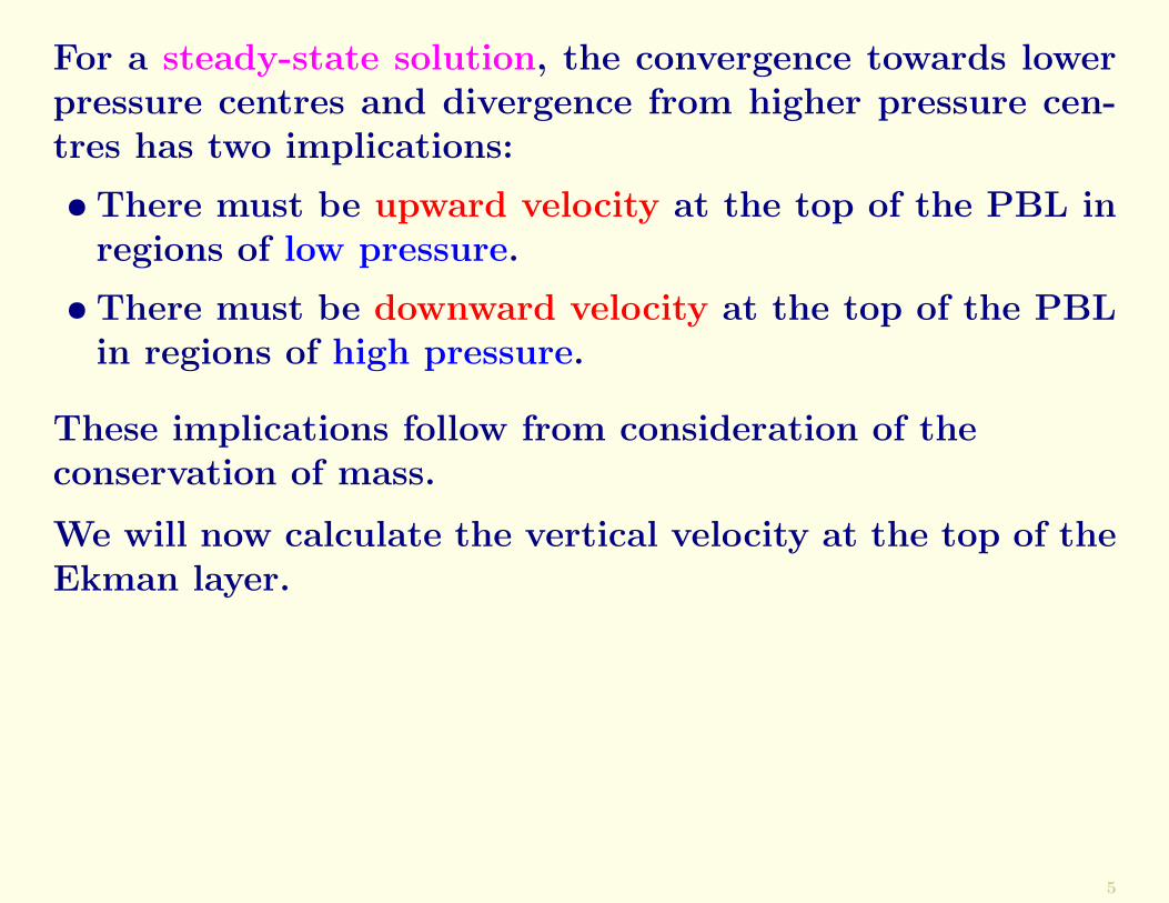
For a steady-state solution, the convergence towards lowerpressure centres and divergence from higher pressure cen-tres has two implications:

• There must be upward velocity at the top of the PBL inregions of low pressure.

5

For a steady-state solution, the convergence towards lowerpressure centres and divergence from higher pressure cen-tres has two implications:

• There must be upward velocity at the top of the PBL inregions of low pressure.

• There must be downward velocity at the top of the PBLin regions of high pressure.

5

For a steady-state solution, the convergence towards lowerpressure centres and divergence from higher pressure cen-tres has two implications:

• There must be upward velocity at the top of the PBL inregions of low pressure.

• There must be downward velocity at the top of the PBLin regions of high pressure.

These implications follow from consideration of theconservation of mass.

5

For a steady-state solution, the convergence towards lowerpressure centres and divergence from higher pressure cen-tres has two implications:

• There must be upward velocity at the top of the PBL inregions of low pressure.

• There must be downward velocity at the top of the PBLin regions of high pressure.

These implications follow from consideration of theconservation of mass.

We will now calculate the vertical velocity at the top of theEkman layer.

5

First, consider a purely zonal geostrophic flow.So the isobars are oriented in an east-west direction.

6

First, consider a purely zonal geostrophic flow.So the isobars are oriented in an east-west direction.

The cross-isober mass transport per unit area in theplanetary boundary layer (PBL) is just ρ0v (kgm−2s−1).

6

First, consider a purely zonal geostrophic flow.So the isobars are oriented in an east-west direction.

The cross-isober mass transport per unit area in theplanetary boundary layer (PBL) is just ρ0v (kgm−2s−1).

The cross-isober mass transport through a column of unitwidth extending through the entire PBL is the vertical in-tegral of ρ0v through the layer z = 0 to z = D = π/γ:

M =

∫ D

0ρ0v dz (kgm−1s−1)

6

First, consider a purely zonal geostrophic flow.So the isobars are oriented in an east-west direction.

The cross-isober mass transport per unit area in theplanetary boundary layer (PBL) is just ρ0v (kgm−2s−1).

The cross-isober mass transport through a column of unitwidth extending through the entire PBL is the vertical in-tegral of ρ0v through the layer z = 0 to z = D = π/γ:

M =

∫ D

0ρ0v dz (kgm−1s−1)

Now substitute the Ekman solution for v:

v = uge−γz sin(γz) = uge

−πz/D sin(πz/D)

6

First, consider a purely zonal geostrophic flow.So the isobars are oriented in an east-west direction.

The cross-isober mass transport per unit area in theplanetary boundary layer (PBL) is just ρ0v (kgm−2s−1).

The cross-isober mass transport through a column of unitwidth extending through the entire PBL is the vertical in-tegral of ρ0v through the layer z = 0 to z = D = π/γ:

M =

∫ D

0ρ0v dz (kgm−1s−1)

Now substitute the Ekman solution for v:

v = uge−γz sin(γz) = uge

−πz/D sin(πz/D)

The result is thus

M =

∫ D

0ρ0ug exp(−πz/D) sin(πz/D) dz

6

Since ρ0 and ug are assumed to be constant, we have

M = ρ0ug

∫ D

0exp(−πz/D) sin(πz/D) dz

7

Since ρ0 and ug are assumed to be constant, we have

M = ρ0ug

∫ D

0exp(−πz/D) sin(πz/D) dz

Defining a new vertical variable Z = πz/D, this is

M = ρ0ug

(D

π

) ∫ π

0exp(−Z) sin Z dZ

7

Since ρ0 and ug are assumed to be constant, we have

M = ρ0ug

∫ D

0exp(−πz/D) sin(πz/D) dz

Defining a new vertical variable Z = πz/D, this is

M = ρ0ug

(D

π

) ∫ π

0exp(−Z) sin Z dZ

Using a standard integral, this may be written

M = 12

(D

π

)ρ0ug

7

Since ρ0 and ug are assumed to be constant, we have

M = ρ0ug

∫ D

0exp(−πz/D) sin(πz/D) dz

Defining a new vertical variable Z = πz/D, this is

M = ρ0ug

(D

π

) ∫ π

0exp(−Z) sin Z dZ

Using a standard integral, this may be written

M = 12

(D

π

)ρ0ug

Here we have used the fact that

e−π ≈ 0.0432 � 1

7

Exercise: Show that∫ π

0exp(−Z) sin Z dz = 1

2(1 + e−π) ≈ 12

8

Exercise: Show that∫ π

0exp(−Z) sin Z dz = 1

2(1 + e−π) ≈ 12

Solution:• Evaluate the integral analytically

• Consult a Table of Integrals (e.g., GR2.663)

• Evaluate by numerical integration (MatLab)

• Use Maple to evaluate it.

8

Exercise: Show that∫ π

0exp(−Z) sin Z dz = 1

2(1 + e−π) ≈ 12

Solution:• Evaluate the integral analytically

• Consult a Table of Integrals (e.g., GR2.663)

• Evaluate by numerical integration (MatLab)

• Use Maple to evaluate it.

Note that the analytical evaluation of the integral is straight-forward.

8

Exercise: Show that∫ π

0exp(−Z) sin Z dz = 1

2(1 + e−π) ≈ 12

Solution:• Evaluate the integral analytically

• Consult a Table of Integrals (e.g., GR2.663)

• Evaluate by numerical integration (MatLab)

• Use Maple to evaluate it.

Note that the analytical evaluation of the integral is straight-forward.

For example, it can be done by means of integration byparts (twice), or by expressing the sin-function in terms ofcomplex exponentials.

8

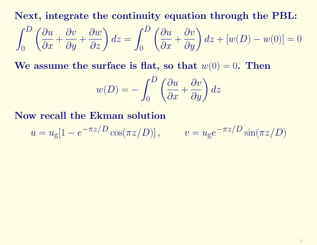
Next, integrate the continuity equation through the PBL:∫ D

0

(∂u

∂x+

∂v

∂y+

∂w

∂z

)dz =

∫ D

0

(∂u

∂x+

∂v

∂y

)dz + [w(D)− w(0)] = 0

9

Next, integrate the continuity equation through the PBL:∫ D

0

(∂u

∂x+

∂v

∂y+

∂w

∂z

)dz =

∫ D

0

(∂u

∂x+

∂v

∂y

)dz + [w(D)− w(0)] = 0

We assume the surface is flat, so that w(0) = 0. Then

w(D) = −∫ D

0

(∂u

∂x+

∂v

∂y

)dz

9

Next, integrate the continuity equation through the PBL:∫ D

0

(∂u

∂x+

∂v

∂y+

∂w

∂z

)dz =

∫ D

0

(∂u

∂x+

∂v

∂y

)dz + [w(D)− w(0)] = 0

We assume the surface is flat, so that w(0) = 0. Then

w(D) = −∫ D

0

(∂u

∂x+

∂v

∂y

)dz

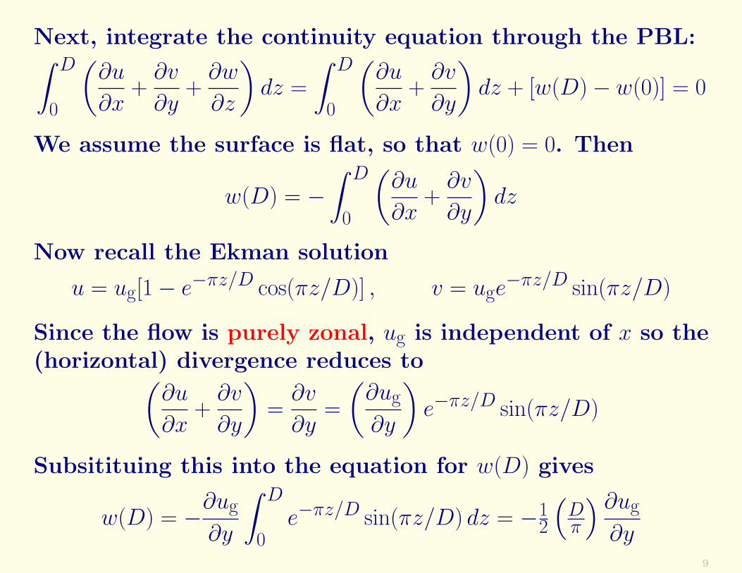
Now recall the Ekman solution

u = ug[1− e−πz/D cos(πz/D)] , v = uge−πz/D sin(πz/D)

9

Next, integrate the continuity equation through the PBL:∫ D

0

(∂u

∂x+

∂v

∂y+

∂w

∂z

)dz =

∫ D

0

(∂u

∂x+

∂v

∂y

)dz + [w(D)− w(0)] = 0

We assume the surface is flat, so that w(0) = 0. Then

w(D) = −∫ D

0

(∂u

∂x+

∂v

∂y

)dz

Now recall the Ekman solution

u = ug[1− e−πz/D cos(πz/D)] , v = uge−πz/D sin(πz/D)

Since the flow is purely zonal, ug is independent of x so the(horizontal) divergence reduces to(

∂u

∂x+

∂v

∂y

)=

∂v

∂y=

(∂ug

∂y

)e−πz/D sin(πz/D)

9

Next, integrate the continuity equation through the PBL:∫ D

0

(∂u

∂x+

∂v

∂y+

∂w

∂z

)dz =

∫ D

0

(∂u

∂x+

∂v

∂y

)dz + [w(D)− w(0)] = 0

We assume the surface is flat, so that w(0) = 0. Then

w(D) = −∫ D

0

(∂u

∂x+

∂v

∂y

)dz

Now recall the Ekman solution

u = ug[1− e−πz/D cos(πz/D)] , v = uge−πz/D sin(πz/D)

Since the flow is purely zonal, ug is independent of x so the(horizontal) divergence reduces to(

∂u

∂x+

∂v

∂y

)=

∂v

∂y=

(∂ug

∂y

)e−πz/D sin(πz/D)

Subsitituing this into the equation for w(D) gives

w(D) = −∂ug

∂y

∫ D

0e−πz/D sin(πz/D) dz = −1

2

(Dπ

) ∂ug

∂y9

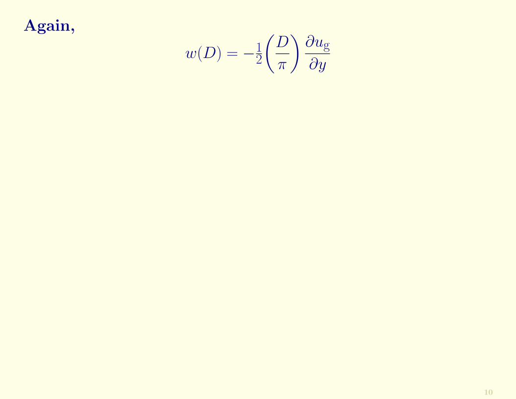
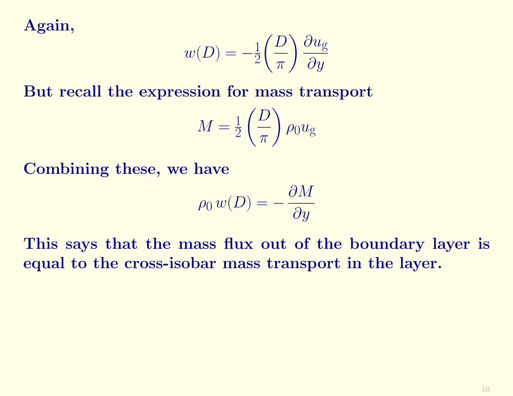
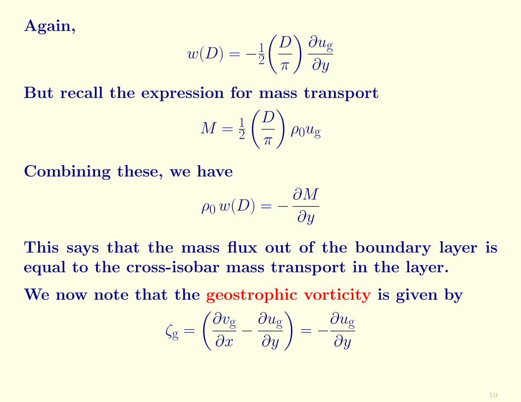
Again,

w(D) = −12

(D

π

)∂ug

∂y

10

Again,

w(D) = −12

(D

π

)∂ug

∂y

But recall the expression for mass transport

M = 12

(D

π

)ρ0ug

10

Again,

w(D) = −12

(D

π

)∂ug

∂y

But recall the expression for mass transport

M = 12

(D

π

)ρ0ug

Combining these, we have

ρ0 w(D) = − ∂M

∂y

10

Again,

w(D) = −12

(D

π

)∂ug

∂y

But recall the expression for mass transport

M = 12

(D

π

)ρ0ug

Combining these, we have

ρ0 w(D) = − ∂M

∂y

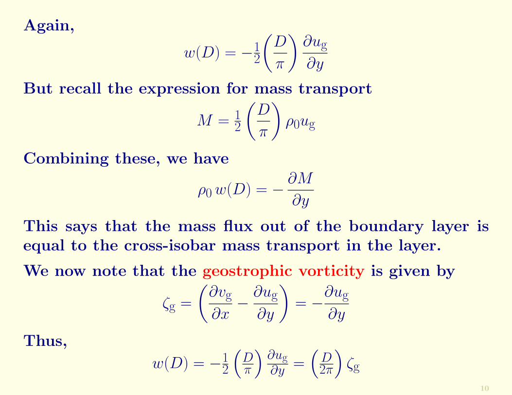
This says that the mass flux out of the boundary layer isequal to the cross-isobar mass transport in the layer.

10

Again,

w(D) = −12

(D

π

)∂ug

∂y

But recall the expression for mass transport

M = 12

(D

π

)ρ0ug

Combining these, we have

ρ0 w(D) = − ∂M

∂y

This says that the mass flux out of the boundary layer isequal to the cross-isobar mass transport in the layer.

We now note that the geostrophic vorticity is given by

ζg =

(∂vg

∂x−

∂ug

∂y

)= −

∂ug

∂y

10

Again,

w(D) = −12

(D

π

)∂ug

∂y

But recall the expression for mass transport

M = 12

(D

π

)ρ0ug

Combining these, we have

ρ0 w(D) = − ∂M

∂y

This says that the mass flux out of the boundary layer isequal to the cross-isobar mass transport in the layer.

We now note that the geostrophic vorticity is given by

ζg =

(∂vg

∂x−

∂ug

∂y

)= −

∂ug

∂y

Thus,

w(D) = −12

(Dπ

)∂ug∂y =

(D2π

)ζg

10

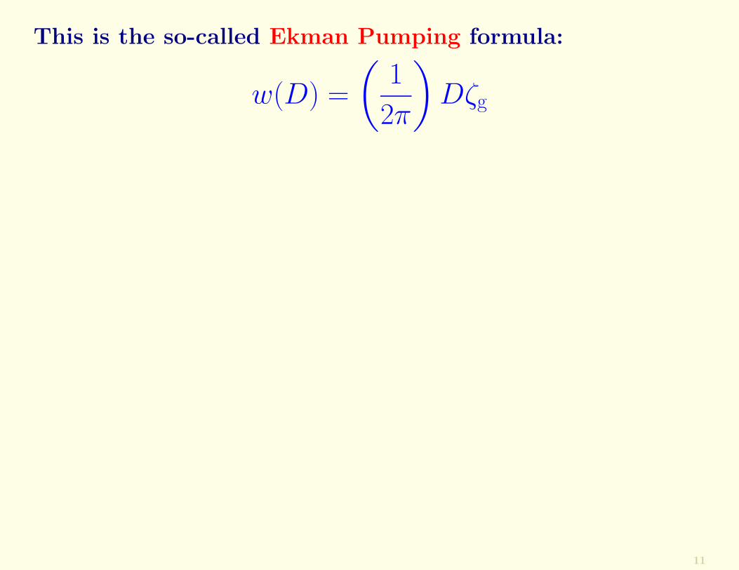
This is the so-called Ekman Pumping formula:

w(D) =

(1

2π

)Dζg

11

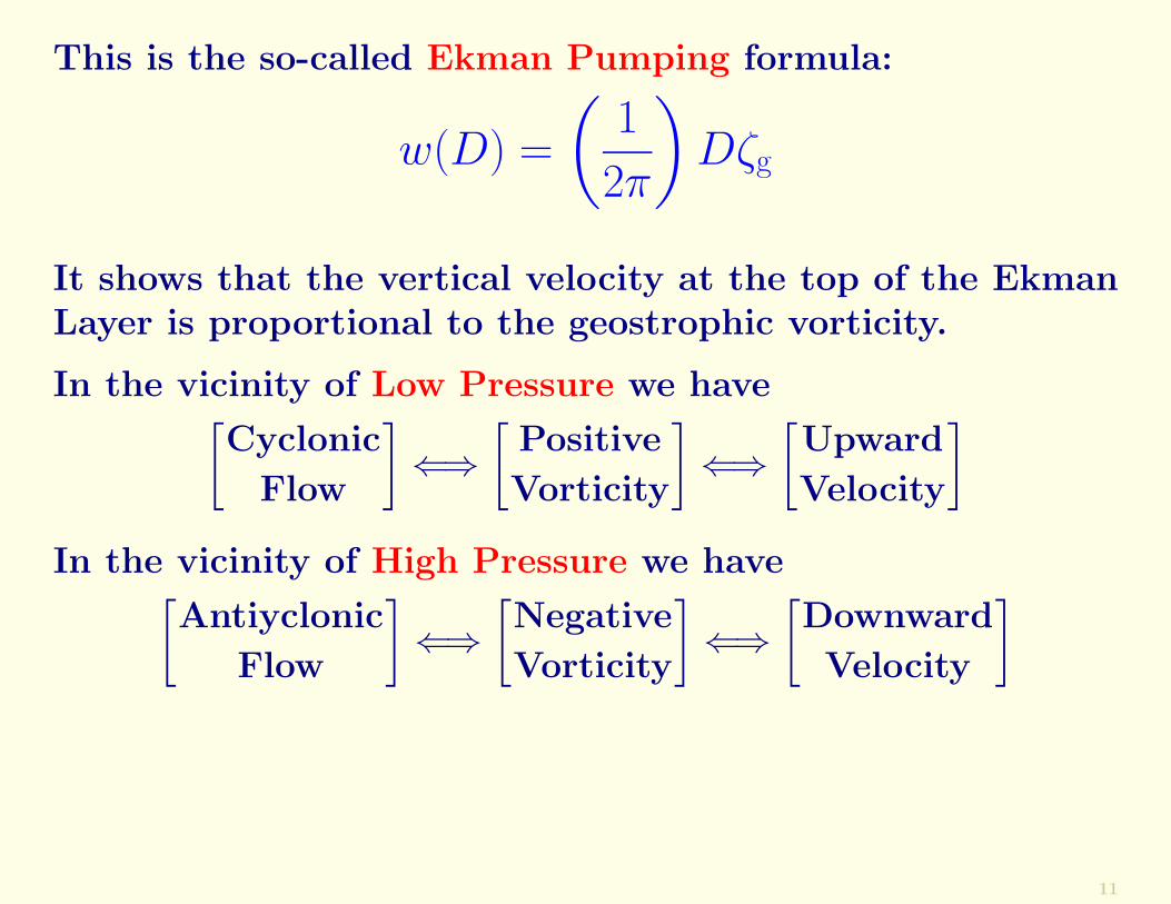
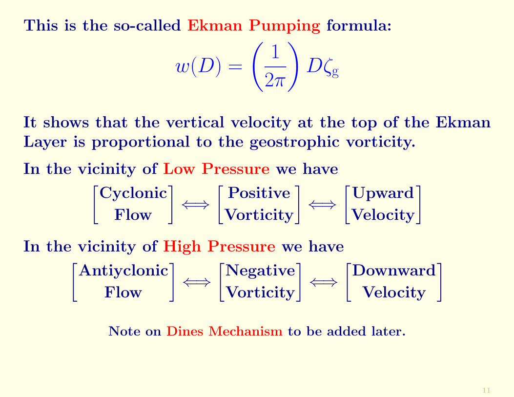
This is the so-called Ekman Pumping formula:

w(D) =

(1

2π

)Dζg

It shows that the vertical velocity at the top of the EkmanLayer is proportional to the geostrophic vorticity.

11

This is the so-called Ekman Pumping formula:

w(D) =

(1

2π

)Dζg

It shows that the vertical velocity at the top of the EkmanLayer is proportional to the geostrophic vorticity.

In the vicinity of Low Pressure we have[Cyclonic

Flow

]⇐⇒

[Positive

Vorticity

]⇐⇒

[Upward

Velocity

]

11

This is the so-called Ekman Pumping formula:

w(D) =

(1

2π

)Dζg

It shows that the vertical velocity at the top of the EkmanLayer is proportional to the geostrophic vorticity.

In the vicinity of Low Pressure we have[Cyclonic

Flow

]⇐⇒

[Positive

Vorticity

]⇐⇒

[Upward

Velocity

]In the vicinity of High Pressure we have[

Antiyclonic

Flow

]⇐⇒

[Negative

Vorticity

]⇐⇒

[Downward

Velocity

]

11

This is the so-called Ekman Pumping formula:

w(D) =

(1

2π

)Dζg

It shows that the vertical velocity at the top of the EkmanLayer is proportional to the geostrophic vorticity.

In the vicinity of Low Pressure we have[Cyclonic

Flow

]⇐⇒

[Positive

Vorticity

]⇐⇒

[Upward

Velocity

]In the vicinity of High Pressure we have[

Antiyclonic

Flow

]⇐⇒

[Negative

Vorticity

]⇐⇒

[Downward

Velocity

]Note on Dines Mechanism to be added later.

11

Magnitude of Ekman Pumping

12

Magnitude of Ekman PumpingThe vertical velocity is

w(D) =

(1

2π

)Dζg

12

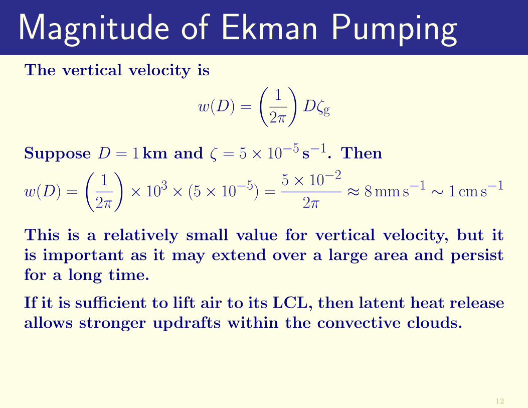
Magnitude of Ekman PumpingThe vertical velocity is

w(D) =

(1

2π

)Dζg

Suppose D = 1km and ζ = 5× 10−5 s−1. Then

w(D) =

(1

2π

)× 103 × (5× 10−5) =

5× 10−2

2π≈ 8 mm s−1 ∼ 1 cm s−1

12

Magnitude of Ekman PumpingThe vertical velocity is

w(D) =

(1

2π

)Dζg

Suppose D = 1km and ζ = 5× 10−5 s−1. Then

w(D) =

(1

2π

)× 103 × (5× 10−5) =

5× 10−2

2π≈ 8 mm s−1 ∼ 1 cm s−1

This is a relatively small value for vertical velocity, but itis important as it may extend over a large area and persistfor a long time.

12

Magnitude of Ekman PumpingThe vertical velocity is

w(D) =

(1

2π

)Dζg

Suppose D = 1km and ζ = 5× 10−5 s−1. Then

w(D) =

(1

2π

)× 103 × (5× 10−5) =

5× 10−2

2π≈ 8 mm s−1 ∼ 1 cm s−1

This is a relatively small value for vertical velocity, but itis important as it may extend over a large area and persistfor a long time.

If it is sufficient to lift air to its LCL, then latent heat releaseallows stronger updrafts within the convective clouds.

12

Storms in Teacups

Standing waves in a tea cup, induced by the propeller rotation of an

airoplane.13

Cyclostrophic Balanced Rotation

14

Cyclostrophic Balanced RotationWe consider now another flow configuration. We ignore therotation of the earth.

14

Cyclostrophic Balanced RotationWe consider now another flow configuration. We ignore therotation of the earth.

We use cylindrical polar coordinates (r, θ, z) and correspond-ing velocity components (U, V,W ).

14

Cyclostrophic Balanced RotationWe consider now another flow configuration. We ignore therotation of the earth.

We use cylindrical polar coordinates (r, θ, z) and correspond-ing velocity components (U, V,W ).

We consider a cyclostrophically balanced vortex spinning insolid rotation.

14

Cyclostrophic Balanced RotationWe consider now another flow configuration. We ignore therotation of the earth.

We use cylindrical polar coordinates (r, θ, z) and correspond-ing velocity components (U, V,W ).

We consider a cyclostrophically balanced vortex spinning insolid rotation.

That is, the azimuthal velocity depends linearly on the ra-dial distance:

Ug = 0 , Vg = ω r

where ω = θ is the constant angular velocity.

14

Cyclostrophic Balanced RotationWe consider now another flow configuration. We ignore therotation of the earth.

We use cylindrical polar coordinates (r, θ, z) and correspond-ing velocity components (U, V,W ).

We consider a cyclostrophically balanced vortex spinning insolid rotation.

That is, the azimuthal velocity depends linearly on the ra-dial distance:

Ug = 0 , Vg = ω r

where ω = θ is the constant angular velocity.

The centrifugal force is given, as usual, by

V 2

r= ω2r

14

For steady flow, the centrifugal force is balanced by thepressure gradient force:

1

ρ0

∂p

∂r= ω2r

15

For steady flow, the centrifugal force is balanced by thepressure gradient force:

1

ρ0

∂p

∂r= ω2r

This can be integrated immediately to give

p = p0 + 12ρ0ω

2r2

so the surface has the form of a parabola (or more correctlya paraboloid of revolution).

15

For steady flow, the centrifugal force is balanced by thepressure gradient force:

1

ρ0

∂p

∂r= ω2r

This can be integrated immediately to give

p = p0 + 12ρ0ω

2r2

so the surface has the form of a parabola (or more correctlya paraboloid of revolution).

Near the bottom boundary, the flow is slowed by the effectof viscosity. Then, the centrifugal force is insufficient tobalance the pressure gradient force.

15

For steady flow, the centrifugal force is balanced by thepressure gradient force:

1

ρ0

∂p

∂r= ω2r

This can be integrated immediately to give

p = p0 + 12ρ0ω

2r2

so the surface has the form of a parabola (or more correctlya paraboloid of revolution).

Near the bottom boundary, the flow is slowed by the effectof viscosity. Then, the centrifugal force is insufficient tobalance the pressure gradient force.

As a result, there is radial inflow near the bottom. Bycontinuity of mass, this must result in upward motion nearthe centre.

15

For steady flow, the centrifugal force is balanced by thepressure gradient force:

1

ρ0

∂p

∂r= ω2r

This can be integrated immediately to give

p = p0 + 12ρ0ω

2r2

so the surface has the form of a parabola (or more correctlya paraboloid of revolution).

Near the bottom boundary, the flow is slowed by the effectof viscosity. Then, the centrifugal force is insufficient tobalance the pressure gradient force.

As a result, there is radial inflow near the bottom. Bycontinuity of mass, this must result in upward motion nearthe centre.

Furthermore, outflow must occur in the fluid above theboundary layer.

15

16

This secondary circulation is completed by downward flownear the edges of the container.

17

This secondary circulation is completed by downward flownear the edges of the container.

At the bottom surface, the flow must vanish completely.

17

This secondary circulation is completed by downward flownear the edges of the container.

At the bottom surface, the flow must vanish completely.

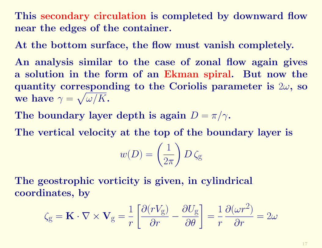
An analysis similar to the case of zonal flow again givesa solution in the form of an Ekman spiral. But now thequantity corresponding to the Coriolis parameter is 2ω, sowe have γ =

√ω/K.

17

This secondary circulation is completed by downward flownear the edges of the container.

At the bottom surface, the flow must vanish completely.

An analysis similar to the case of zonal flow again givesa solution in the form of an Ekman spiral. But now thequantity corresponding to the Coriolis parameter is 2ω, sowe have γ =

√ω/K.

The boundary layer depth is again D = π/γ.

17

This secondary circulation is completed by downward flownear the edges of the container.

At the bottom surface, the flow must vanish completely.

An analysis similar to the case of zonal flow again givesa solution in the form of an Ekman spiral. But now thequantity corresponding to the Coriolis parameter is 2ω, sowe have γ =

√ω/K.

The boundary layer depth is again D = π/γ.

The vertical velocity at the top of the boundary layer is

w(D) =

(1

2π

)D ζg

17

This secondary circulation is completed by downward flownear the edges of the container.

At the bottom surface, the flow must vanish completely.

An analysis similar to the case of zonal flow again givesa solution in the form of an Ekman spiral. But now thequantity corresponding to the Coriolis parameter is 2ω, sowe have γ =

√ω/K.

The boundary layer depth is again D = π/γ.

The vertical velocity at the top of the boundary layer is

w(D) =

(1

2π

)D ζg

The geostrophic vorticity is given, in cylindricalcoordinates, by

ζg = K · ∇ ×Vg =1

r

[∂(rVg)

∂r−

∂Ug

∂θ

]=

1

r

∂(ωr2)

∂r= 2ω

17

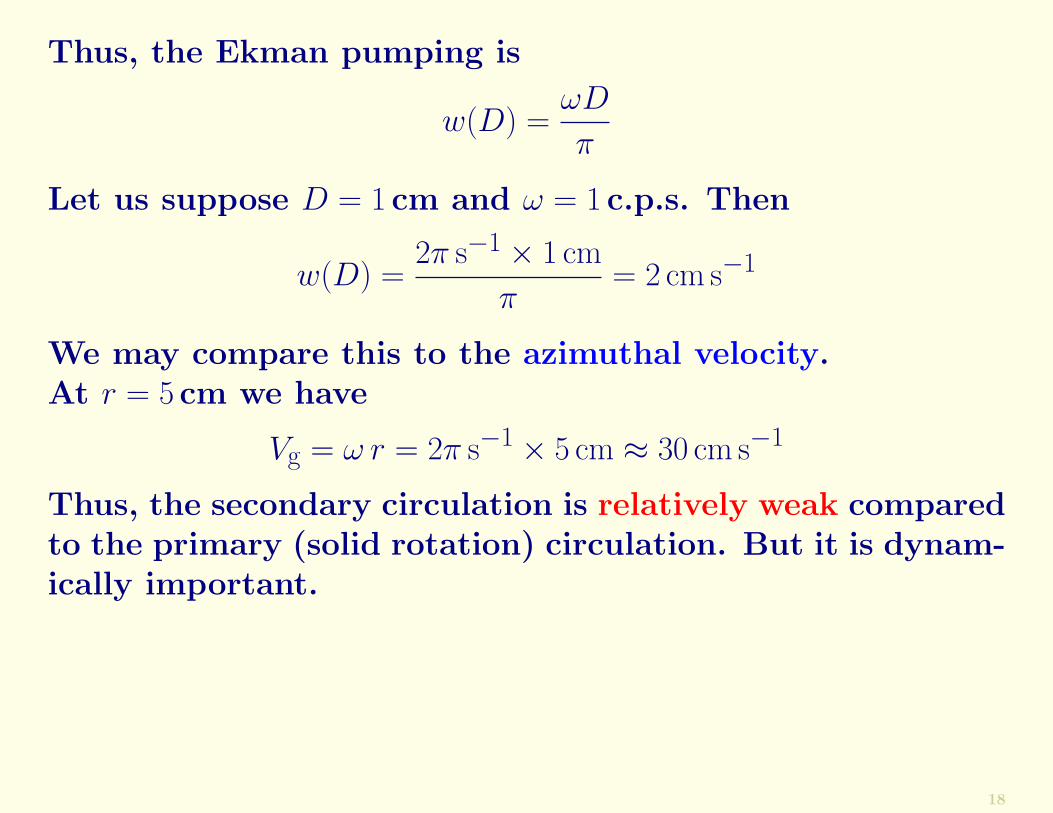
Thus, the Ekman pumping is

w(D) =ωD

π

18

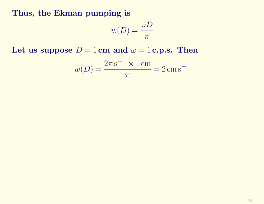
Thus, the Ekman pumping is

w(D) =ωD

π

Let us suppose D = 1 cm and ω = 1 c.p.s. Then

w(D) =2π s−1 × 1 cm

π= 2 cm s−1

18

Thus, the Ekman pumping is

w(D) =ωD

π

Let us suppose D = 1 cm and ω = 1 c.p.s. Then

w(D) =2π s−1 × 1 cm

π= 2 cm s−1

We may compare this to the azimuthal velocity.At r = 5 cm we have

Vg = ω r = 2π s−1 × 5 cm ≈ 30 cm s−1

Thus, the secondary circulation is relatively weak comparedto the primary (solid rotation) circulation. But it is dynam-ically important.

18

Thus, the Ekman pumping is

w(D) =ωD

π

Let us suppose D = 1 cm and ω = 1 c.p.s. Then

w(D) =2π s−1 × 1 cm

π= 2 cm s−1

We may compare this to the azimuthal velocity.At r = 5 cm we have

Vg = ω r = 2π s−1 × 5 cm ≈ 30 cm s−1

Thus, the secondary circulation is relatively weak comparedto the primary (solid rotation) circulation. But it is dynam-ically important.

Exercise: Create a storm in a teacup:Stir your tea (no milk) and observe the leaves.

18

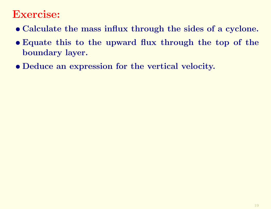
Exercise:• Calculate the mass influx through the sides of a cyclone.

• Equate this to the upward flux through the top of theboundary layer.

• Deduce an expression for the vertical velocity.

19

Exercise:• Calculate the mass influx through the sides of a cyclone.

• Equate this to the upward flux through the top of theboundary layer.

• Deduce an expression for the vertical velocity.

19

Sketch of Solution:

From the Ekman solution, the mean inward velocity is

Vinward = 12ug

(Dπ

)

20

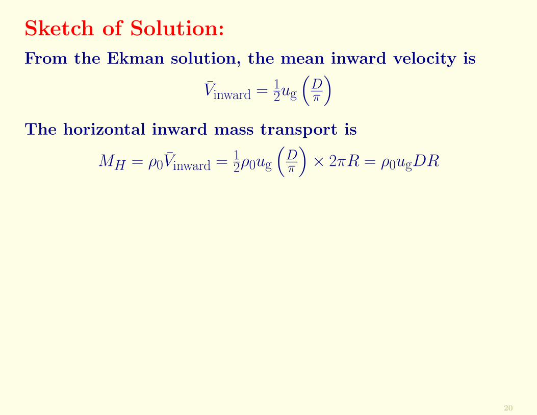
Sketch of Solution:

From the Ekman solution, the mean inward velocity is

Vinward = 12ug

(Dπ

)The horizontal inward mass transport is

MH = ρ0Vinward = 12ρ0ug

(Dπ

)× 2πR = ρ0ugDR

20

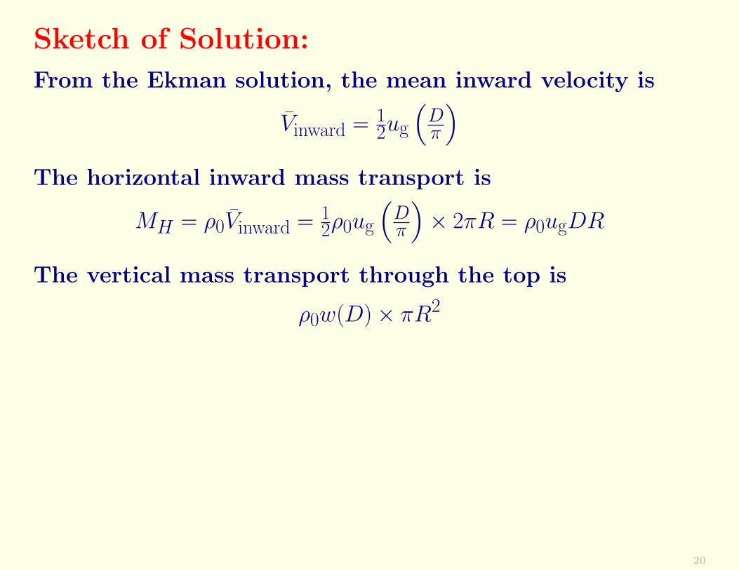
Sketch of Solution:

From the Ekman solution, the mean inward velocity is

Vinward = 12ug

(Dπ

)The horizontal inward mass transport is

MH = ρ0Vinward = 12ρ0ug

(Dπ

)× 2πR = ρ0ugDR

The vertical mass transport through the top is

ρ0w(D)× πR2

20

Sketch of Solution:

From the Ekman solution, the mean inward velocity is

Vinward = 12ug

(Dπ

)The horizontal inward mass transport is

MH = ρ0Vinward = 12ρ0ug

(Dπ

)× 2πR = ρ0ugDR

The vertical mass transport through the top is

ρ0w(D)× πR2

These must be equal, so

w(D) =ρ0ugDR

ρ0 × πR2=

D

πRug

20

Sketch of Solution:

From the Ekman solution, the mean inward velocity is

Vinward = 12ug

(Dπ

)The horizontal inward mass transport is

MH = ρ0Vinward = 12ρ0ug

(Dπ

)× 2πR = ρ0ugDR

The vertical mass transport through the top is

ρ0w(D)× πR2

These must be equal, so

w(D) =ρ0ugDR

ρ0 × πR2=

D

πRug

For solid body rotation, ug = ωR and the geostrophic vortic-ity is ζg = 2ω, so

w(D) =D

2πζg

20

Spin-Down

21

Spin-DownWe estimate the characteristic spin-down time of thesecondary circulation for a barotropic atmosphere.

21

Spin-DownWe estimate the characteristic spin-down time of thesecondary circulation for a barotropic atmosphere.

The barotropic vorticity equation is

dζg

dt= −f

(∂u

∂x+

∂v

∂y

)= f

∂w

∂z

21

Spin-DownWe estimate the characteristic spin-down time of thesecondary circulation for a barotropic atmosphere.

The barotropic vorticity equation is

dζg

dt= −f

(∂u

∂x+

∂v

∂y

)= f

∂w

∂z

We integrate this through the free atmopshere, that is, fromz = D to z = H, where H is the height of the tropopause.

21

Spin-DownWe estimate the characteristic spin-down time of thesecondary circulation for a barotropic atmosphere.

The barotropic vorticity equation is

dζg

dt= −f

(∂u

∂x+

∂v

∂y

)= f

∂w

∂z

We integrate this through the free atmopshere, that is, fromz = D to z = H, where H is the height of the tropopause.

The result is

(H −D)dζg

dt= f [w(H)−W (D)]

21

Spin-DownWe estimate the characteristic spin-down time of thesecondary circulation for a barotropic atmosphere.

The barotropic vorticity equation is

dζg

dt= −f

(∂u

∂x+

∂v

∂y

)= f

∂w

∂z

We integrate this through the free atmopshere, that is, fromz = D to z = H, where H is the height of the tropopause.

The result is

(H −D)dζg

dt= f [w(H)−W (D)]

Assuming w(H) = 0 and substituting the Ekman pumpingfor W (D) we get

dζg

dt= − f

(H −D)

(1

2π

)Dζg

21

Assuming H � D, this is

dζg

dt= − fD

2πHζg

22

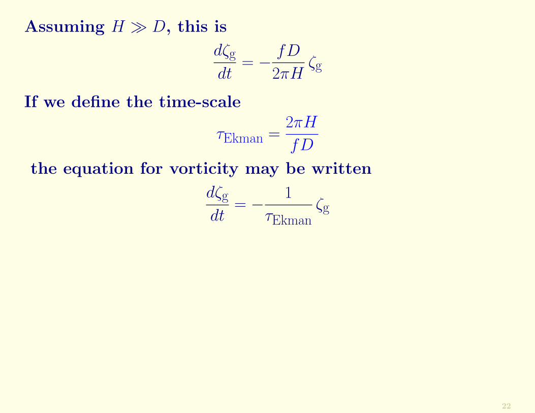
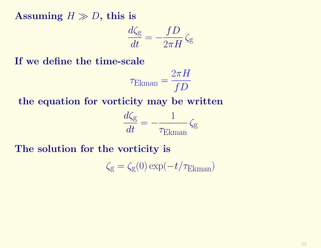
Assuming H � D, this is

dζg

dt= − fD

2πHζg

If we define the time-scale

τEkman =2πH

fD

the equation for vorticity may be written

dζg

dt= − 1

τEkmanζg

22

Assuming H � D, this is

dζg

dt= − fD

2πHζg

If we define the time-scale

τEkman =2πH

fD

the equation for vorticity may be written

dζg

dt= − 1

τEkmanζg

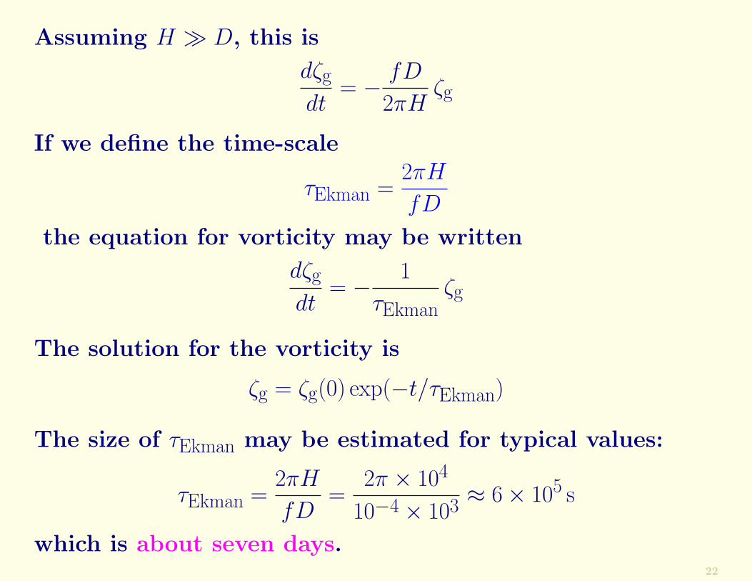
The solution for the vorticity is

ζg = ζg(0) exp(−t/τEkman)

22

Assuming H � D, this is

dζg

dt= − fD

2πHζg

If we define the time-scale

τEkman =2πH

fD

the equation for vorticity may be written

dζg

dt= − 1

τEkmanζg

The solution for the vorticity is

ζg = ζg(0) exp(−t/τEkman)

The size of τEkman may be estimated for typical values:

τEkman =2πH

fD=

2π × 104

10−4 × 103≈ 6× 105 s

which is about seven days.22

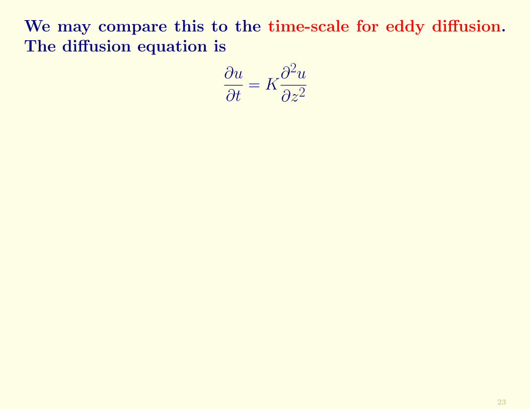
We may compare this to the time-scale for eddy diffusion.The diffusion equation is

∂u

∂t= K

∂2u

∂z2

23

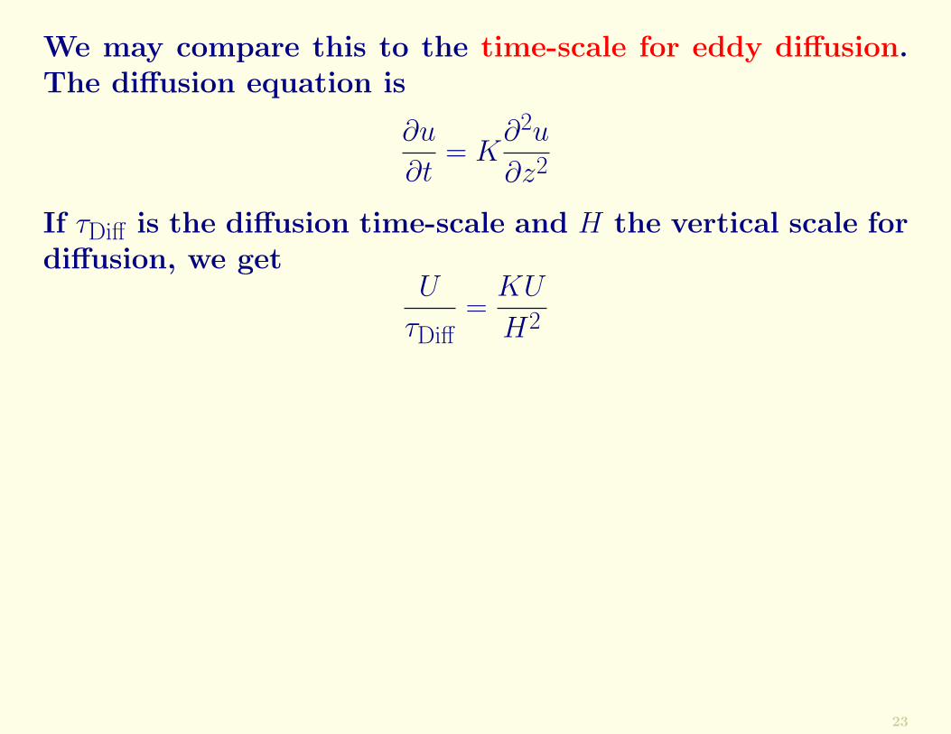
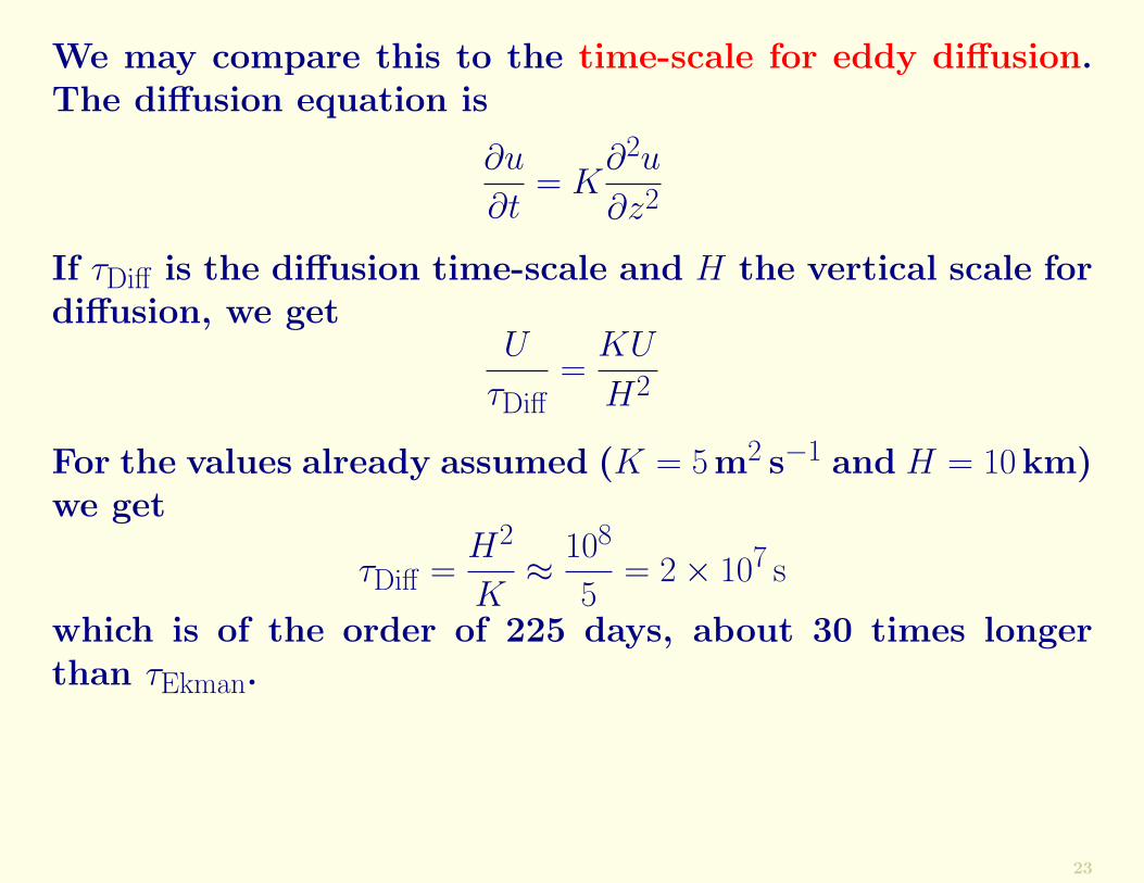
We may compare this to the time-scale for eddy diffusion.The diffusion equation is

∂u

∂t= K

∂2u

∂z2

If τDiff is the diffusion time-scale and H the vertical scale fordiffusion, we get

U

τDiff=

KU

H2

23

We may compare this to the time-scale for eddy diffusion.The diffusion equation is

∂u

∂t= K

∂2u

∂z2

If τDiff is the diffusion time-scale and H the vertical scale fordiffusion, we get

U

τDiff=

KU

H2

For the values already assumed (K = 5m2 s−1 and H = 10km)we get

τDiff =H2

K≈ 108

5= 2× 107 s

which is of the order of 225 days, about 30 times longerthan τEkman.

23

We may compare this to the time-scale for eddy diffusion.The diffusion equation is

∂u

∂t= K

∂2u

∂z2

If τDiff is the diffusion time-scale and H the vertical scale fordiffusion, we get

U

τDiff=

KU

H2

For the values already assumed (K = 5m2 s−1 and H = 10km)we get

τDiff =H2

K≈ 108

5= 2× 107 s

which is of the order of 225 days, about 30 times longerthan τEkman.

Thus, in the absence of convective clouds, Ekman spin-downis much more effective than eddy diffusion.

23

We may compare this to the time-scale for eddy diffusion.The diffusion equation is

∂u

∂t= K

∂2u

∂z2

If τDiff is the diffusion time-scale and H the vertical scale fordiffusion, we get

U

τDiff=

KU

H2

For the values already assumed (K = 5m2 s−1 and H = 10km)we get

τDiff =H2

K≈ 108

5= 2× 107 s

which is of the order of 225 days, about 30 times longerthan τEkman.

Thus, in the absence of convective clouds, Ekman spin-downis much more effective than eddy diffusion.

However, cumulonumbus convection can produce rapid trans-port of heat and momentum through the entire troposphere.

23

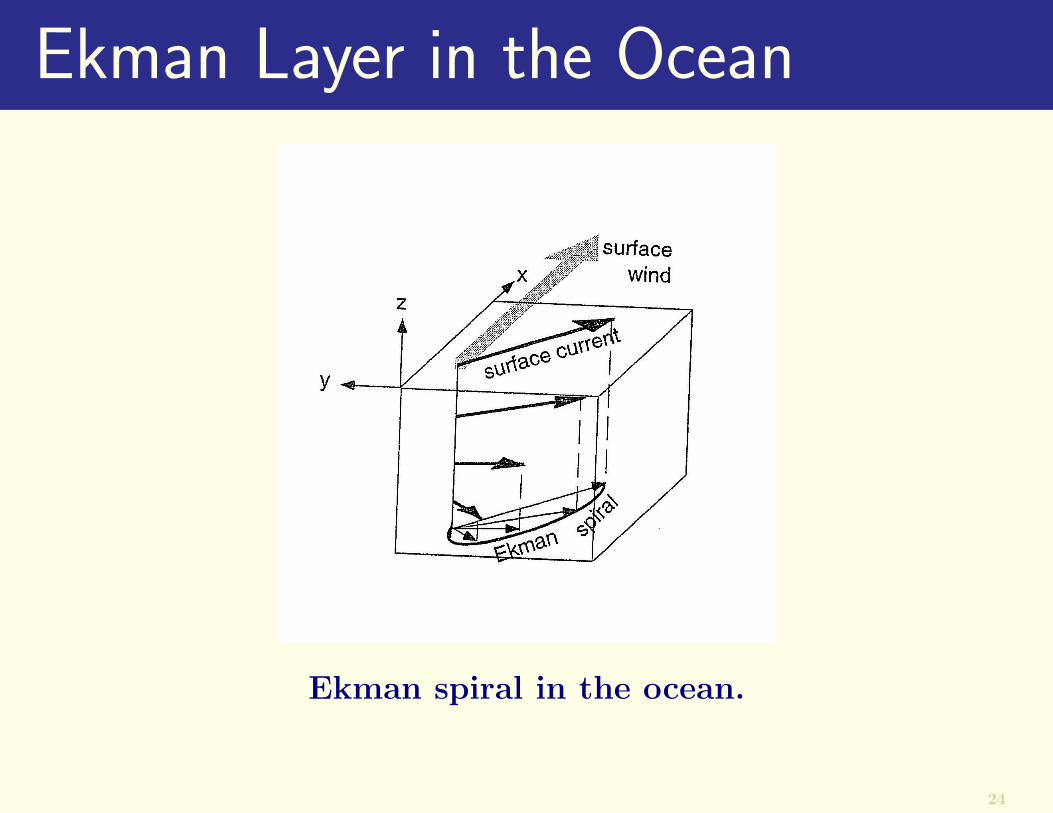
Ekman Layer in the Ocean

Ekman spiral in the ocean.

24

25

Typical La Nina Pattern

Mean sea surface temperature, eastern Pacific Ocean5 September to 5 October, 1998.

26

End of §5.5

27

28