
4.1. Particles as waves Statement Acceptance Light acts as ...
47
4. Wave-like properties of particles 4.1. Particles as waves Statement Acceptance Light acts as waves Common experience Light is made up of photons Seems reasonable Particles are solid, indivisible entities Common experience Particles are waves What ??? Elements of Nuclear Engineering and Radiological Sciences I NERS 311: Slide #1
Transcript of 4.1. Particles as waves Statement Acceptance Light acts as ...
4. Wave-like properties of particles
4.1. Particles as waves
Statement Acceptance
Light acts as waves Common experienceLight is made up of photons Seems reasonableParticles are solid, indivisible entities Common experienceParticles are waves What ???
Elements of Nuclear Engineering and Radiological Sciences I NERS 311: Slide #1
Some nomenclature
symbol meaning
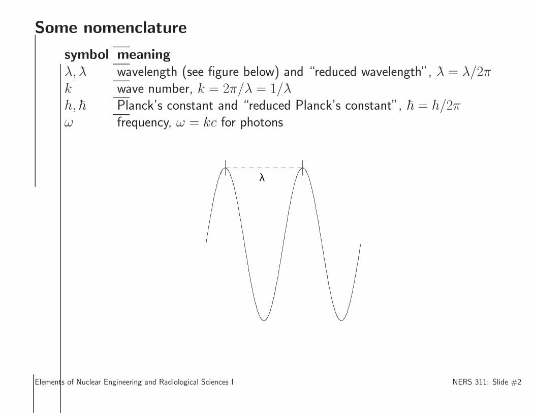
λ, λ wavelength (see figure below) and “reduced wavelength”, λ = λ/2πk wave number, k = 2π/λ = 1/λh, ~ Planck’s constant and “reduced Planck’s constant”, ~ = h/2πω frequency, ω = kc for photons
λ
Elements of Nuclear Engineering and Radiological Sciences I NERS 311: Slide #2
Matter waves...
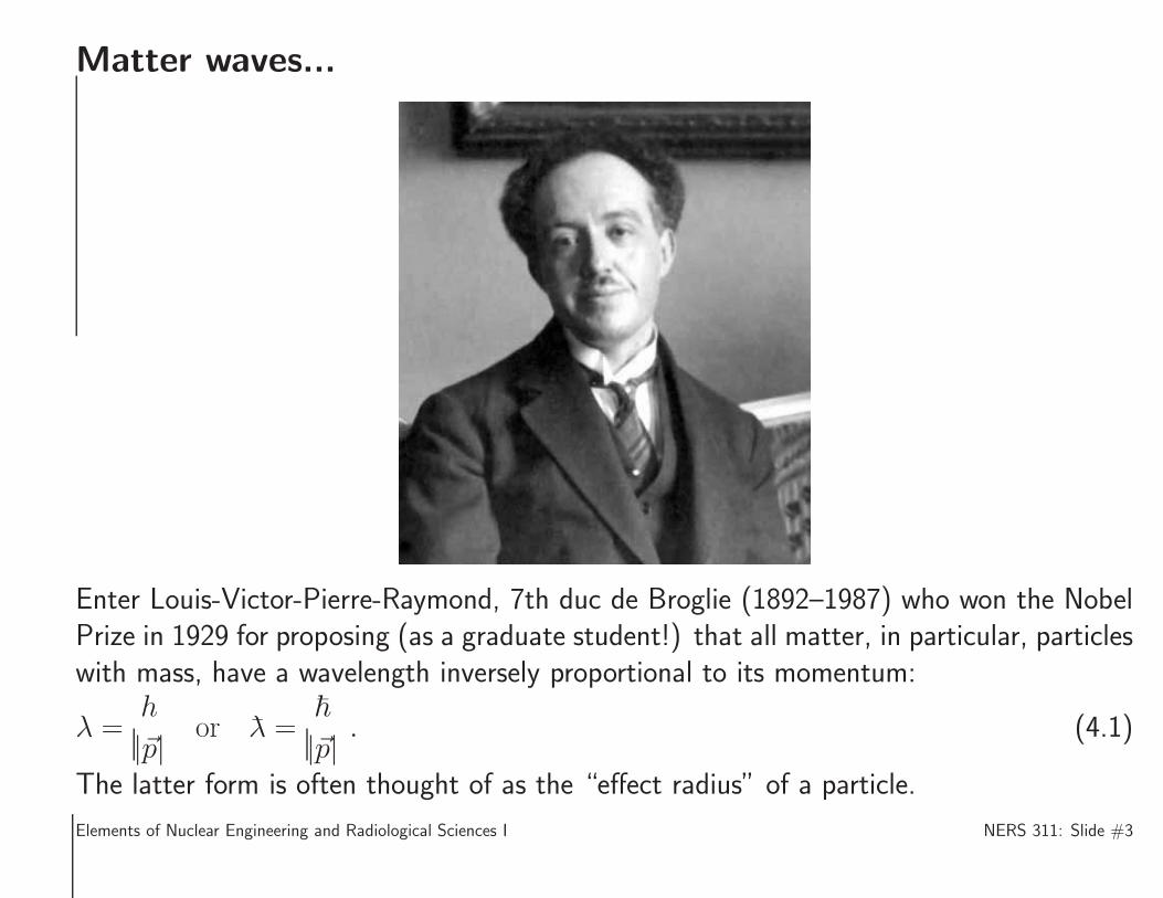
Enter Louis-Victor-Pierre-Raymond, 7th duc de Broglie (1892–1987) who won the NobelPrize in 1929 for proposing (as a graduate student!) that all matter, in particular, particleswith mass, have a wavelength inversely proportional to its momentum:
λ =h
|~p| or λ =~
|~p| . (4.1)
The latter form is often thought of as the “effect radius” of a particle.
Elements of Nuclear Engineering and Radiological Sciences I NERS 311: Slide #3
...Matter waves...
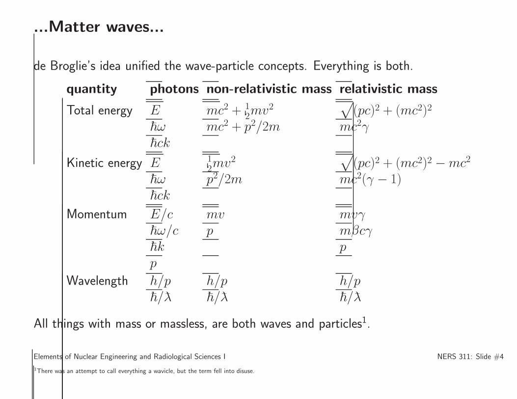
de Broglie’s idea unified the wave-particle concepts. Everything is both.
quantity photons non-relativistic mass relativistic mass
Total energy E mc2 + 12mv2
√
(pc)2 + (mc2)2
~ω mc2 + p2/2m mc2γ~ck
Kinetic energy E 12mv2
√
(pc)2 + (mc2)2 −mc2
~ω p2/2m mc2(γ − 1)~ck
Momentum E/c mv mvγ~ω/c p mβcγ~k pp
Wavelength h/p h/p h/p~/λ ~/λ ~/λ
All things with mass or massless, are both waves and particles1.
Elements of Nuclear Engineering and Radiological Sciences I NERS 311: Slide #4
1There was an attempt to call everything a wavicle, but the term fell into disuse.
...Matter waves...
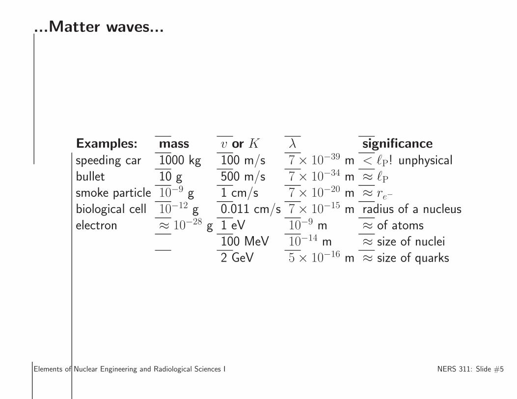
Examples: mass v or K λ significance
speeding car 1000 kg 100 m/s 7× 10−39 m < ℓP! unphysicalbullet 10 g 500 m/s 7× 10⁻³⁴ m ≈ ℓPsmoke particle 10−9 g 1 cm/s 7× 10⁻²⁰ m ≈ re−biological cell 10−12 g 0.011 cm/s 7× 10⁻¹⁵ m radius of a nucleuselectron ≈ 10−28 g 1 eV 10−9 m ≈ of atoms
100 MeV 10−14 m ≈ size of nuclei2 GeV 5× 10⁻¹⁶ m ≈ size of quarks
Elements of Nuclear Engineering and Radiological Sciences I NERS 311: Slide #5
...Matter waves
The first 3 examples in the previous table produce unphysical distances. The Plancklength, ℓP = 1.61619926× 10⁻³⁵ m, is the assumed granularity of space.
A comparison of the next two would yield no practical information.
However, as soon as we can get a fundamental particle to wavelength of the order of otherfundamental particles, we can measure some useful information about them.
The math to describe this is a little involved, and involves Fourier transforms, which wewill describe shortly. The full description of how electrons may be used as probes of nucleiand quarks will come in NERS 312.
Some of these numbers are mind-boggling small.
Other mind-boggling numbers:Age of the universe, in seconds: 3× 10¹⁷
Bill Gates’ fortune in $s: 80× 109
Bill has made 3¢s per day, since the start of the universe!
Elements of Nuclear Engineering and Radiological Sciences I NERS 311: Slide #6
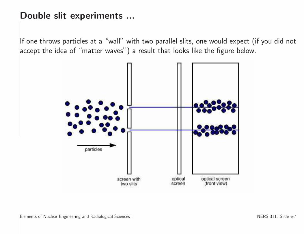
Double slit experiments ...
If one throws particles at a “wall” with two parallel slits, one would expect (if you did notaccept the idea of “matter waves”) a result that looks like the figure below.
Elements of Nuclear Engineering and Radiological Sciences I NERS 311: Slide #7
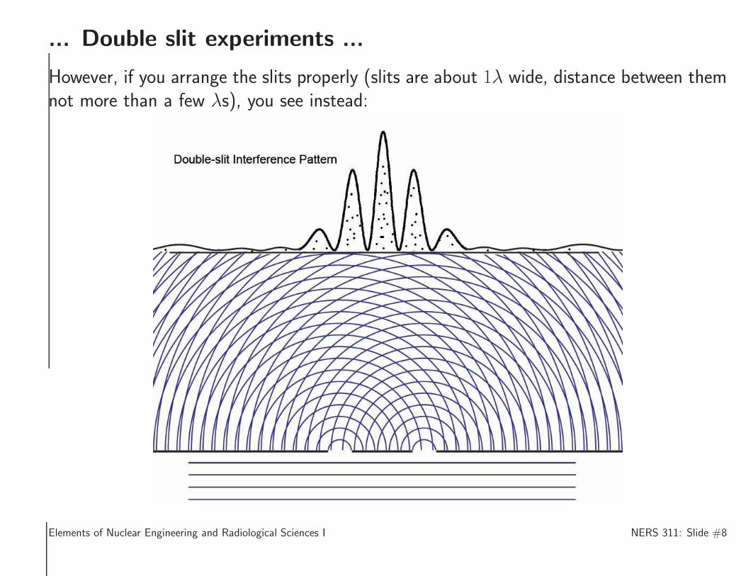
... Double slit experiments ...
However, if you arrange the slits properly (slits are about 1λ wide, distance between themnot more than a few λs), you see instead:
Elements of Nuclear Engineering and Radiological Sciences I NERS 311: Slide #8
... Double slit experiments
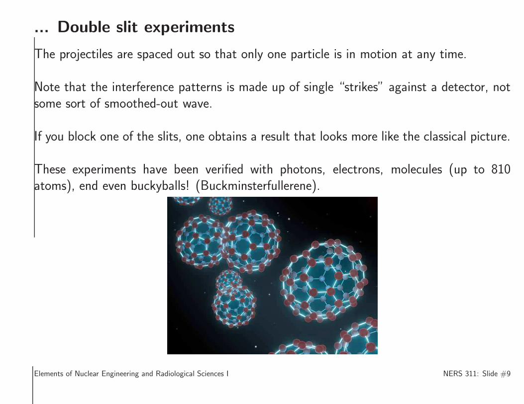
The projectiles are spaced out so that only one particle is in motion at any time.
Note that the interference patterns is made up of single “strikes” against a detector, notsome sort of smoothed-out wave.
If you block one of the slits, one obtains a result that looks more like the classical picture.
These experiments have been verified with photons, electrons, molecules (up to 810atoms), end even buckyballs! (Buckminsterfullerene).
Elements of Nuclear Engineering and Radiological Sciences I NERS 311: Slide #9
Waves, composites, superposition, and Fourier transforms ...
We have encountered an expression for a monochromatic (one energy) wave previously, inChapter 3. Let us generalize the notation:
A monochromatic plane wave traveling along the z-axis is:
A(z, t) = A0ei[k0z−ω(k0)t] , (4.2)
where A(z, t) is the amplitude in space and time and A0 represents the amplitude of thewave number k0 component of this wave.
The direction of motion is given by the sign of k0. If k0 is positive, it is traveling downthe +z-axis. If k0 is negative, it is traveling down the -z-axis.
ω is still the frequency, but here, for generality, we allow it to be a function of k. Forexample, ω = c|k| for photons. ω must always be positive, because ~ω is the energy ofthe wave. This applies for all types of particles.
Elements of Nuclear Engineering and Radiological Sciences I NERS 311: Slide #10
...Waves, composites, superposition, and Fourier transforms ...
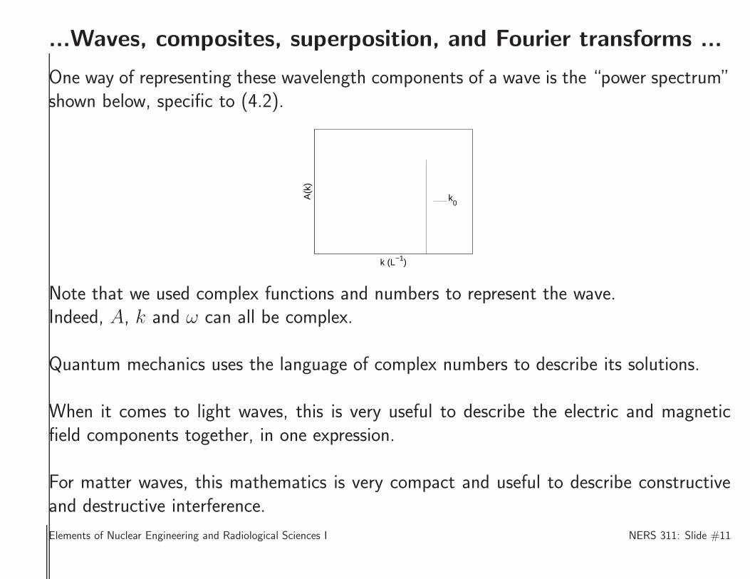
One way of representing these wavelength components of a wave is the “power spectrum”shown below, specific to (4.2).
k (L−1)
A(k
)
k0
Note that we used complex functions and numbers to represent the wave.Indeed, A, k and ω can all be complex.
Quantum mechanics uses the language of complex numbers to describe its solutions.
When it comes to light waves, this is very useful to describe the electric and magneticfield components together, in one expression.
For matter waves, this mathematics is very compact and useful to describe constructiveand destructive interference.
Elements of Nuclear Engineering and Radiological Sciences I NERS 311: Slide #11
...Waves, composites, superposition, and Fourier transforms ...
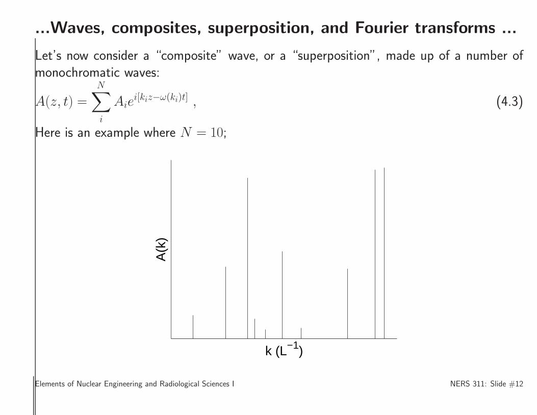
Let’s now consider a “composite” wave, or a “superposition”, made up of a number ofmonochromatic waves:
A(z, t) =N∑
i
Aiei[kiz−ω(ki)t] , (4.3)
Here is an example where N = 10;
k (L−1)
A(k
)
Elements of Nuclear Engineering and Radiological Sciences I NERS 311: Slide #12
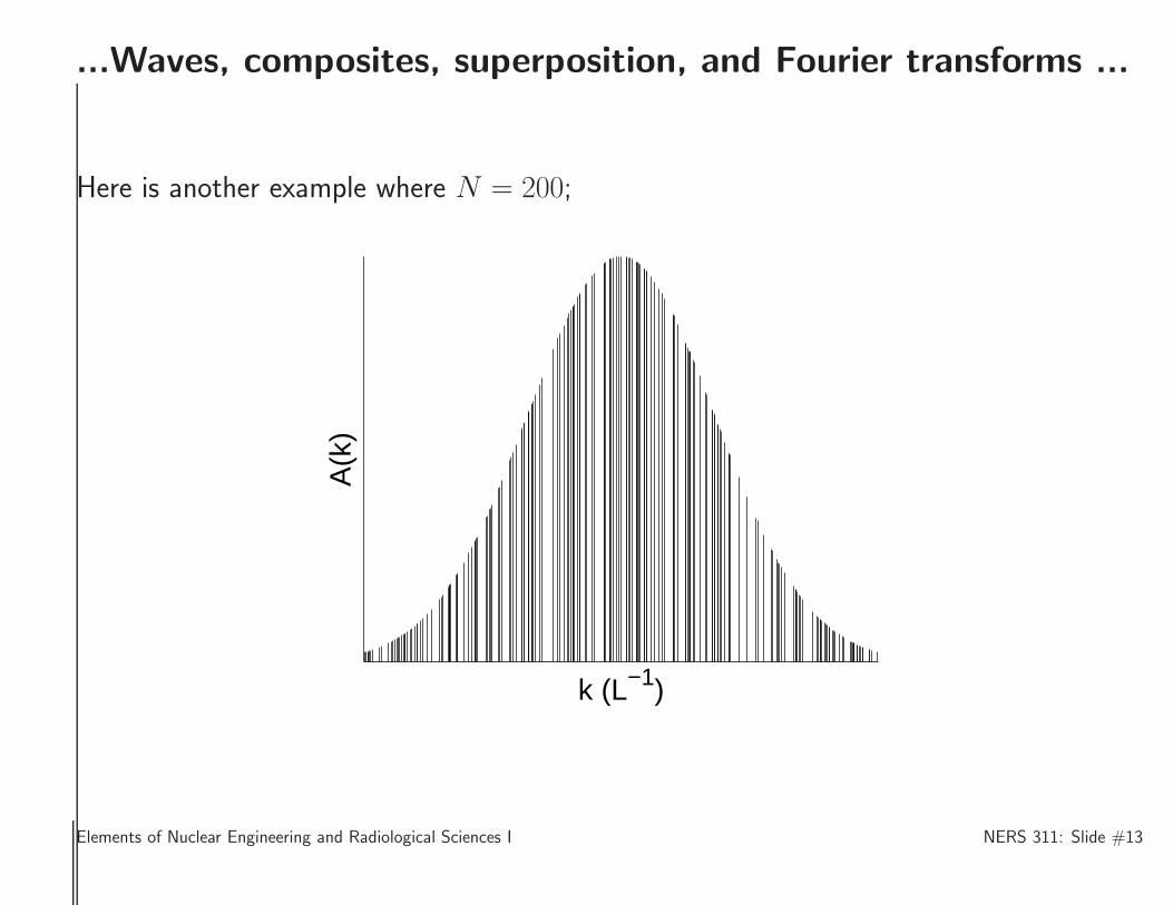
...Waves, composites, superposition, and Fourier transforms ...
Here is another example where N = 200;
k (L−1)
A(k
)
Elements of Nuclear Engineering and Radiological Sciences I NERS 311: Slide #13
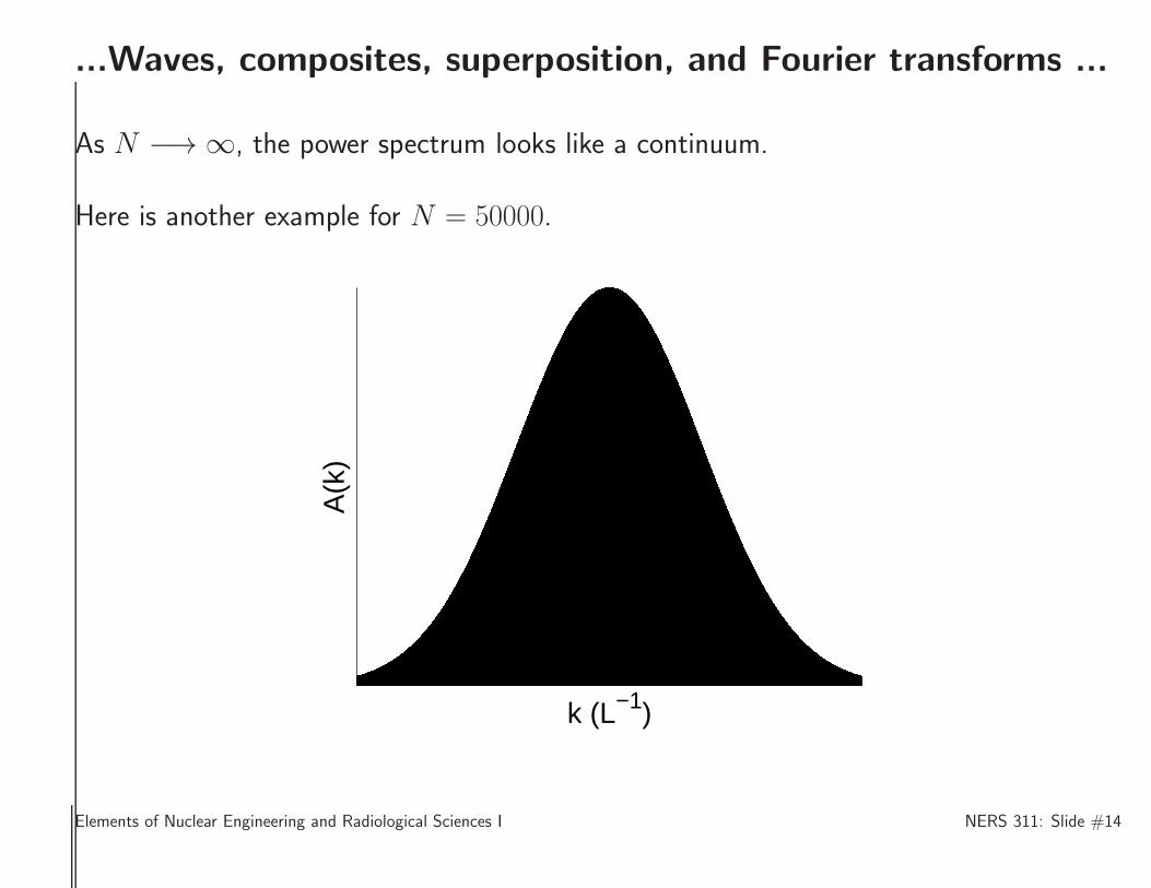
...Waves, composites, superposition, and Fourier transforms ...
As N −→ ∞, the power spectrum looks like a continuum.
Here is another example for N = 50000.
k (L−1)
A(k
)
Elements of Nuclear Engineering and Radiological Sciences I NERS 311: Slide #14
...Waves, composites, superposition, and Fourier transforms ...
In 1D, the amplitude of a wave that has a continuum of frequencies, is given by a“Fourier transform”:
A(z, t) =1
(2π)1/2
∫ +∞
−∞dk A(k)ei[kz−ω(k)t] . (4.4)
Note that the limits of integration suggest that this continuum composite is made up ofcomponents moving to the right, as well as to the left.
We also can recover (4.2) by specifying:
A(k) = (2π)1/2A0δ(k − k0) , (4.5)
and (4.3) by specifying:
A(k) = (2π)1/2Aiδ(k − ki) for i = 1, 2, 3, . . . N . (4.6)
Elements of Nuclear Engineering and Radiological Sciences I NERS 311: Slide #15
An aside on the Dirac delta function, δ(x− x0) ...
... as well as the Kronecker delta and the Heaviside step function.
Dirac’s δ-function is a mathematical tool for extracting the value of a function at a givenpoint, viz.∫ x2
x1
dx δ(x− x0)f(x) = f(x0), if x1 ≤ x0 ≤ x2 . (4.7)
If x0 is outside the range of integration, the integral is 0.
The Heaviside step function:
θ(x− x0) = 1, if x ≥ x0= 0, if x < x0 (4.8)
It is easily shown that the indefinite integral of the Dirac δ is the step function.∫ x
−∞dx δ(x− x0) = θ(x− x0) (4.9)
Elements of Nuclear Engineering and Radiological Sciences I NERS 311: Slide #16
An aside on the Dirac delta function, δ(x− x0) ...
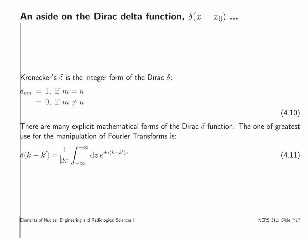
Kronecker’s δ is the integer form of the Dirac δ:
δmn = 1, if m = n
= 0, if m 6= n
(4.10)
There are many explicit mathematical forms of the Dirac δ-function. The one of greatestuse for the manipulation of Fourier Transforms is:
δ(k − k′) =1
2π
∫ +∞
−∞dz e±i(k−k′)z (4.11)
Elements of Nuclear Engineering and Radiological Sciences I NERS 311: Slide #17
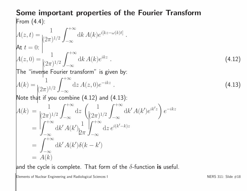
Some important properties of the Fourier TransformFrom (4.4):
A(z, t) =1
(2π)1/2
∫ +∞
−∞dk A(k)ei[kz−ω(k)t] .
At t = 0:
A(z, 0) =1
(2π)1/2
∫ +∞
−∞dk A(k)eikz . (4.12)
The “inverse Fourier transform” is given by:
A(k) =1
(2π)1/2
∫ +∞
−∞dz A(z, 0)e−ikz . (4.13)
Note that if you combine (4.12) and (4.13):
A(k) =1
(2π)1/2
∫ +∞
−∞dz
(
1
(2π)1/2
∫ +∞
−∞dk′A(k′)eik
′z)
e−ikz
=
∫ +∞
−∞dk′A(k′)
1
2π
∫ +∞
−∞dz ei(k
′−k)z
=
∫ +∞
−∞dk′A(k′)δ(k − k′)
= A(k)
and the cycle is complete. That form of the δ-function is useful.
Elements of Nuclear Engineering and Radiological Sciences I NERS 311: Slide #18
An example ...
As an example, let’s make:
A(k) = A0θ(k + k0)θ(k0 − k) . (4.14)
It can be shown2:
A(z, 0) =
(
2
π
)1/2
A0
(
sin k0z
z
)
. (4.15)
On the next page is illustrated an example with different values of k0.
Elements of Nuclear Engineering and Radiological Sciences I NERS 311: Slide #19
2The Mathematica code for this is: Integrate[A0/Sqrt[2 Pi] Exp[-i k z], {k,-k0,k0}]
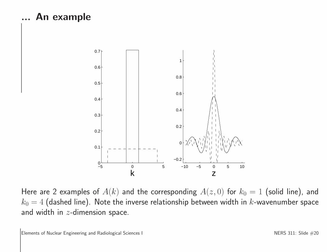
... An example
−5 0 50
0.1
0.2
0.3
0.4
0.5
0.6
0.7
k−10 −5 0 5 10
−0.2
0
0.2
0.4
0.6
0.8
1
z
Here are 2 examples of A(k) and the corresponding A(z, 0) for k0 = 1 (solid line), andk0 = 4 (dashed line). Note the inverse relationship between width in k-wavenumber spaceand width in z-dimension space.
Elements of Nuclear Engineering and Radiological Sciences I NERS 311: Slide #20
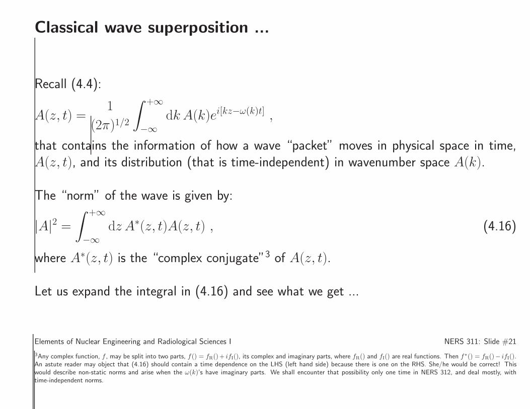
Classical wave superposition ...
Recall (4.4):
A(z, t) =1
(2π)1/2
∫ +∞
−∞dk A(k)ei[kz−ω(k)t] ,
that contains the information of how a wave “packet” moves in physical space in time,A(z, t), and its distribution (that is time-independent) in wavenumber space A(k).
The “norm” of the wave is given by:
|A|2 =∫ +∞
−∞dz A∗(z, t)A(z, t) , (4.16)
where A∗(z, t) is the “complex conjugate”3 of A(z, t).
Let us expand the integral in (4.16) and see what we get ...
Elements of Nuclear Engineering and Radiological Sciences I NERS 311: Slide #21
3Any complex function, f , may be split into two parts, f() = fR()+ ifI(), its complex and imaginary parts, where fR() and fI() are real functions. Then f∗() = fR()− ifI().An astute reader may object that (4.16) should contain a time dependence on the LHS (left hand side) because there is one on the RHS. She/he would be correct! Thiswould describe non-static norms and arise when the ω(k)’s have imaginary parts. We shall encounter that possibility only one time in NERS 312, and deal mostly, withtime-independent norms.
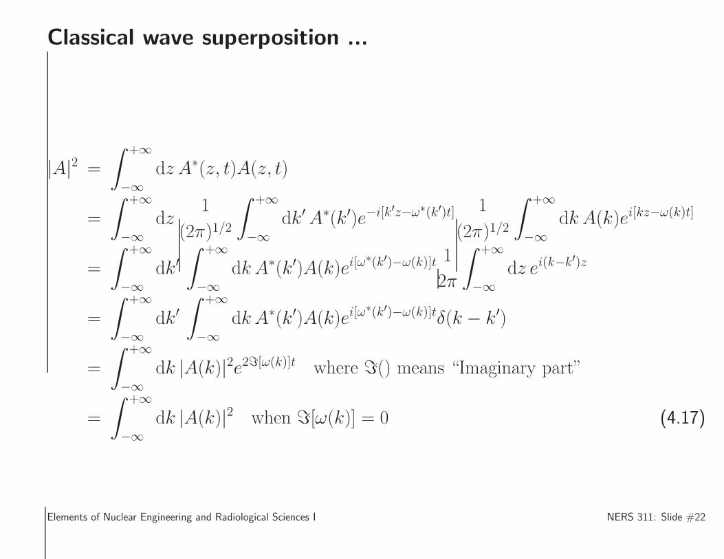
Classical wave superposition ...
|A|2 =
∫ +∞
−∞dz A∗(z, t)A(z, t)
=
∫ +∞
−∞dz
1
(2π)1/2
∫ +∞
−∞dk′A∗(k′)e−i[k′z−ω∗(k′)t] 1
(2π)1/2
∫ +∞
−∞dk A(k)ei[kz−ω(k)t]
=
∫ +∞
−∞dk′
∫ +∞
−∞dk A∗(k′)A(k)ei[ω
∗(k′)−ω(k)]t 1
2π
∫ +∞
−∞dz ei(k−k′)z
=
∫ +∞
−∞dk′
∫ +∞
−∞dk A∗(k′)A(k)ei[ω
∗(k′)−ω(k)]tδ(k − k′)
=
∫ +∞
−∞dk |A(k)|2e2ℑ[ω(k)]t where ℑ() means “Imaginary part”
=
∫ +∞
−∞dk |A(k)|2 when ℑ[ω(k)] = 0 (4.17)
Elements of Nuclear Engineering and Radiological Sciences I NERS 311: Slide #22
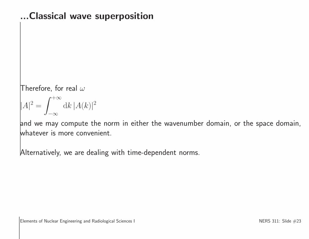
...Classical wave superposition
Therefore, for real ω
|A|2 =∫ +∞
−∞dk |A(k)|2
and we may compute the norm in either the wavenumber domain, or the space domain,whatever is more convenient.
Alternatively, we are dealing with time-dependent norms.
Elements of Nuclear Engineering and Radiological Sciences I NERS 311: Slide #23
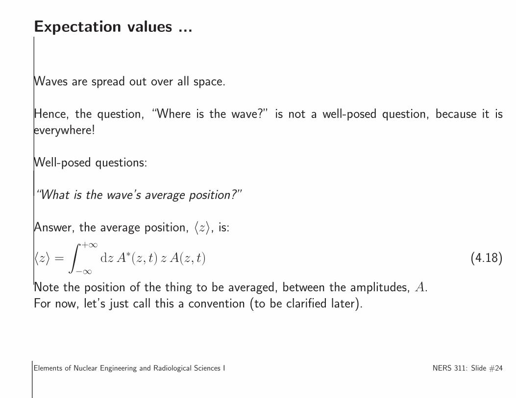
Expectation values ...
Waves are spread out over all space.
Hence, the question, “Where is the wave?” is not a well-posed question, because it iseverywhere!
Well-posed questions:
“What is the wave’s average position?”
Answer, the average position, 〈z〉, is:
〈z〉 =∫ +∞
−∞dz A∗(z, t) z A(z, t) (4.18)
Note the position of the thing to be averaged, between the amplitudes, A.For now, let’s just call this a convention (to be clarified later).
Elements of Nuclear Engineering and Radiological Sciences I NERS 311: Slide #24
...Expectation values ...
“What is the average spread of the wave?”
Answer, the average spread, ∆z, that is defined by:
∆z =√
〈z2〉 − 〈z〉2 (4.19)
where
〈z2〉 =∫ +∞
−∞dz A∗(z, t) z2A(z, t) , (4.20)
and 〈z〉 is given by (4.18).
Elements of Nuclear Engineering and Radiological Sciences I NERS 311: Slide #25
...Expectation values ...
“What is the average wavenumber of the wave?”
The average wavenumber, 〈k〉, can be obtained by:
〈k〉 =∫ +∞
−∞dz A∗(z, t)
(
−i∂
∂z
)
A(z, t) (4.21)
where, after some “inspired intuition”, it is realized that the function that extracts thewavenumber in z-space is a differential operator, that operates to the right, on the waveamplitude A(z, t).
The proof is obtained from substituting for A∗(z, t) and A(z, t) in the above, and grindingout a result, that seems, in retrospect, obvious.
This moderately long derivation is given on the next page.
Elements of Nuclear Engineering and Radiological Sciences I NERS 311: Slide #26
...Expectation values ...
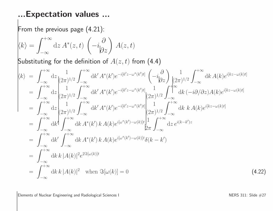
From the previous page (4.21):
〈k〉 =∫ +∞
−∞dz A∗(z, t)
(
−i∂
∂z
)
A(z, t)
Substituting for the definition of A(z, t) from (4.4)
〈k〉 =
∫ +∞
−∞dz
1
(2π)1/2
∫ +∞
−∞dk′A∗(k′)e−i[k′z−ω∗(k′)t]
(
−i∂
∂z
)
1
(2π)1/2
∫ +∞
−∞dk A(k)ei[kz−ω(k)t]
=
∫ +∞
−∞dz
1
(2π)1/2
∫ +∞
−∞dk′A∗(k′)e−i[k′z−ω∗(k′)t] 1
(2π)1/2
∫ +∞
−∞dk (−i∂/∂z)A(k)ei[kz−ω(k)t]
=
∫ +∞
−∞dz
1
(2π)1/2
∫ +∞
−∞dk′A∗(k′)e−i[k′z−ω∗(k′)t] 1
(2π)1/2
∫ +∞
−∞dk k A(k)ei[kz−ω(k)t]
=
∫ +∞
−∞dk′
∫ +∞
−∞dk A∗(k′) k A(k)ei[ω
∗(k′)−ω(k)]t 1
2π
∫ +∞
−∞dz ei(k−k′)z
=
∫ +∞
−∞dk′
∫ +∞
−∞dk A∗(k′) k A(k)ei[ω
∗(k′)−ω(k)]tδ(k − k′)
=
∫ +∞
−∞dk k |A(k)|2e2ℑ[ω(k)]t
=
∫ +∞
−∞dk k |A(k)|2 when ℑ[ω(k)] = 0 (4.22)
Elements of Nuclear Engineering and Radiological Sciences I NERS 311: Slide #27
...Expectation values ...
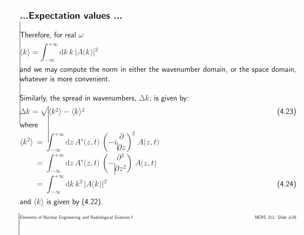
Therefore, for real ω
〈k〉 =∫ +∞
−∞dk k |A(k)|2
and we may compute the norm in either the wavenumber domain, or the space domain,whatever is more convenient.
Similarly, the spread in wavenumbers, ∆k, is given by:
∆k =√
〈k2〉 − 〈k〉2 (4.23)
where
〈k2〉 =
∫ +∞
−∞dz A∗(z, t)
(
−i∂
∂z
)2
A(z, t)
=
∫ +∞
−∞dz A∗(z, t)
(
− ∂2
∂z2
)
A(z, t)
=
∫ +∞
−∞dk k2 |A(k)|2 (4.24)
and 〈k〉 is given by (4.22).
Elements of Nuclear Engineering and Radiological Sciences I NERS 311: Slide #28
...Expectation values ...
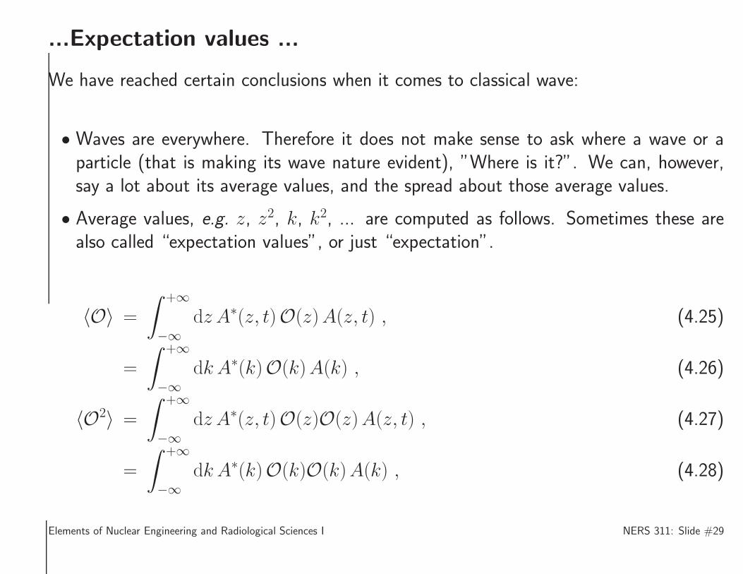
We have reached certain conclusions when it comes to classical wave:
• Waves are everywhere. Therefore it does not make sense to ask where a wave or aparticle (that is making its wave nature evident), ”Where is it?”. We can, however,say a lot about its average values, and the spread about those average values.
• Average values, e.g. z, z2, k, k2, ... are computed as follows. Sometimes these arealso called “expectation values”, or just “expectation”.
〈O〉 =
∫ +∞
−∞dz A∗(z, t)O(z)A(z, t) , (4.25)
=
∫ +∞
−∞dk A∗(k)O(k)A(k) , (4.26)
〈O2〉 =
∫ +∞
−∞dz A∗(z, t)O(z)O(z)A(z, t) , (4.27)
=
∫ +∞
−∞dk A∗(k)O(k)O(k)A(k) , (4.28)
Elements of Nuclear Engineering and Radiological Sciences I NERS 311: Slide #29
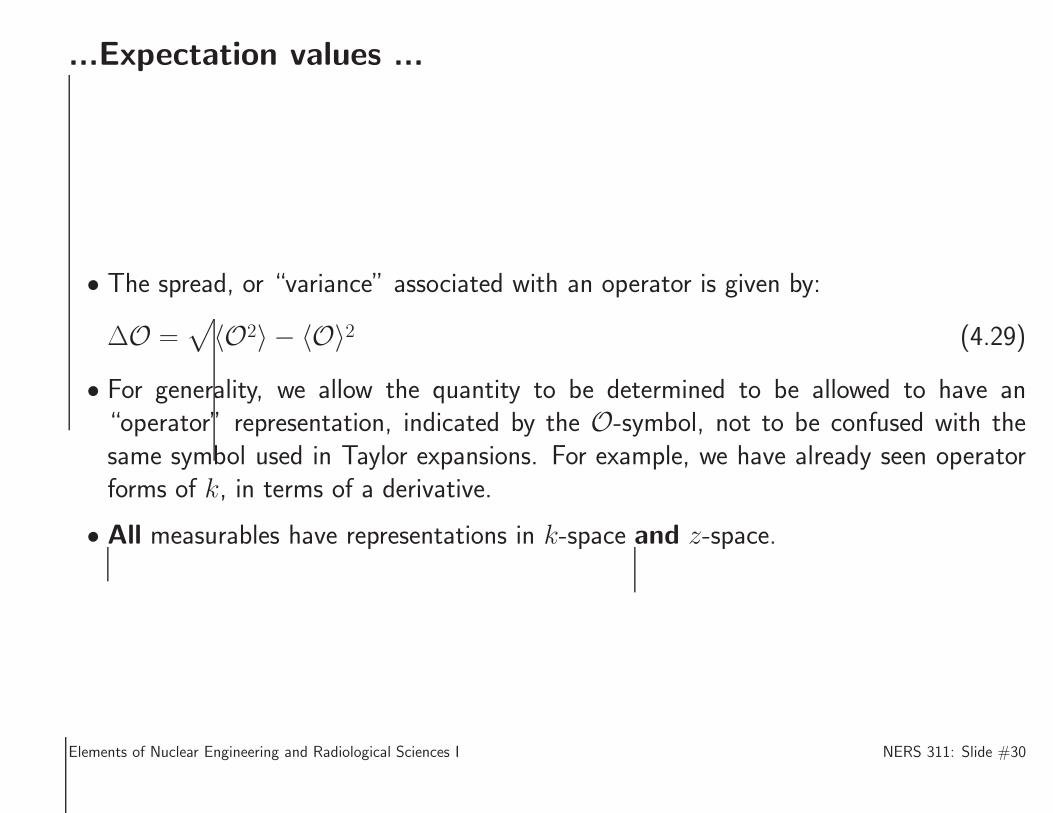
...Expectation values ...
• The spread, or “variance” associated with an operator is given by:
∆O =√
〈O2〉 − 〈O〉2 (4.29)
• For generality, we allow the quantity to be determined to be allowed to have an“operator” representation, indicated by the O-symbol, not to be confused with thesame symbol used in Taylor expansions. For example, we have already seen operatorforms of k, in terms of a derivative.
• All measurables have representations in k-space and z-space.
Elements of Nuclear Engineering and Radiological Sciences I NERS 311: Slide #30
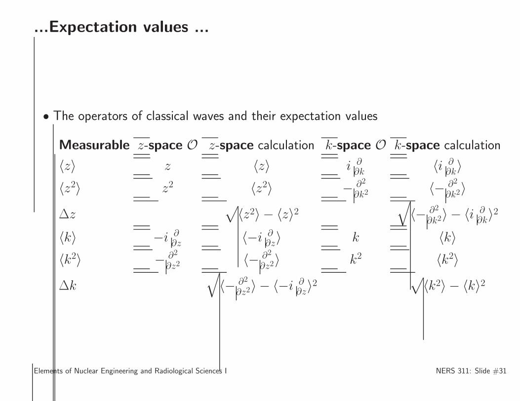
...Expectation values ...
• The operators of classical waves and their expectation values
Measurable z-space O z-space calculation k-space O k-space calculation
〈z〉 z 〈z〉 i ∂∂k
〈i ∂∂k〉
〈z2〉 z2 〈z2〉 − ∂2
∂k2〈− ∂2
∂k2〉
∆z√
〈z2〉 − 〈z〉2√
〈− ∂2
∂k2〉 − 〈i ∂
∂k〉2
〈k〉 −i ∂∂z 〈−i ∂
∂z〉 k 〈k〉〈k2〉 − ∂2
∂z2〈− ∂2
∂z2〉 k2 〈k2〉
∆k√
〈− ∂2
∂z2〉 − 〈−i ∂
∂z〉2
√
〈k2〉 − 〈k〉2
Elements of Nuclear Engineering and Radiological Sciences I NERS 311: Slide #31
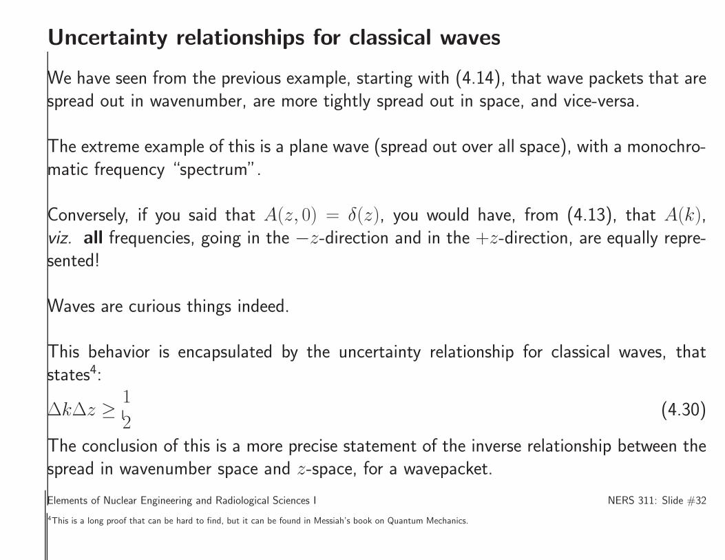
Uncertainty relationships for classical waves
We have seen from the previous example, starting with (4.14), that wave packets that arespread out in wavenumber, are more tightly spread out in space, and vice-versa.
The extreme example of this is a plane wave (spread out over all space), with a monochro-matic frequency “spectrum”.
Conversely, if you said that A(z, 0) = δ(z), you would have, from (4.13), that A(k),viz. all frequencies, going in the −z-direction and in the +z-direction, are equally repre-sented!
Waves are curious things indeed.
This behavior is encapsulated by the uncertainty relationship for classical waves, thatstates4:
∆k∆z ≥ 1
2(4.30)
The conclusion of this is a more precise statement of the inverse relationship between thespread in wavenumber space and z-space, for a wavepacket.
Elements of Nuclear Engineering and Radiological Sciences I NERS 311: Slide #32
4This is a long proof that can be hard to find, but it can be found in Messiah’s book on Quantum Mechanics.
Example of a wavepacket...
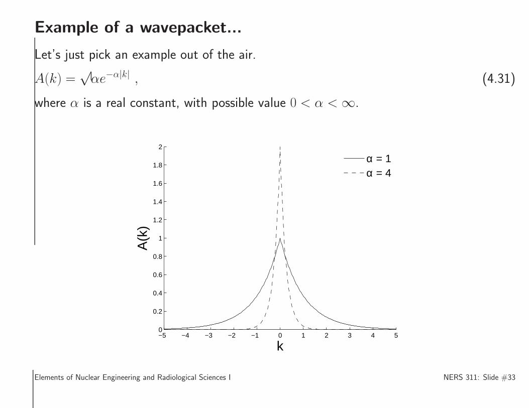
Let’s just pick an example out of the air.
A(k) =√αe−α|k| , (4.31)
where α is a real constant, with possible value 0 < α < ∞.
−5 −4 −3 −2 −1 0 1 2 3 4 50
0.2
0.4
0.6
0.8
1
1.2
1.4
1.6
1.8
2
k
A(k
)
α = 1α = 4
Elements of Nuclear Engineering and Radiological Sciences I NERS 311: Slide #33
... Example of a wavepacket
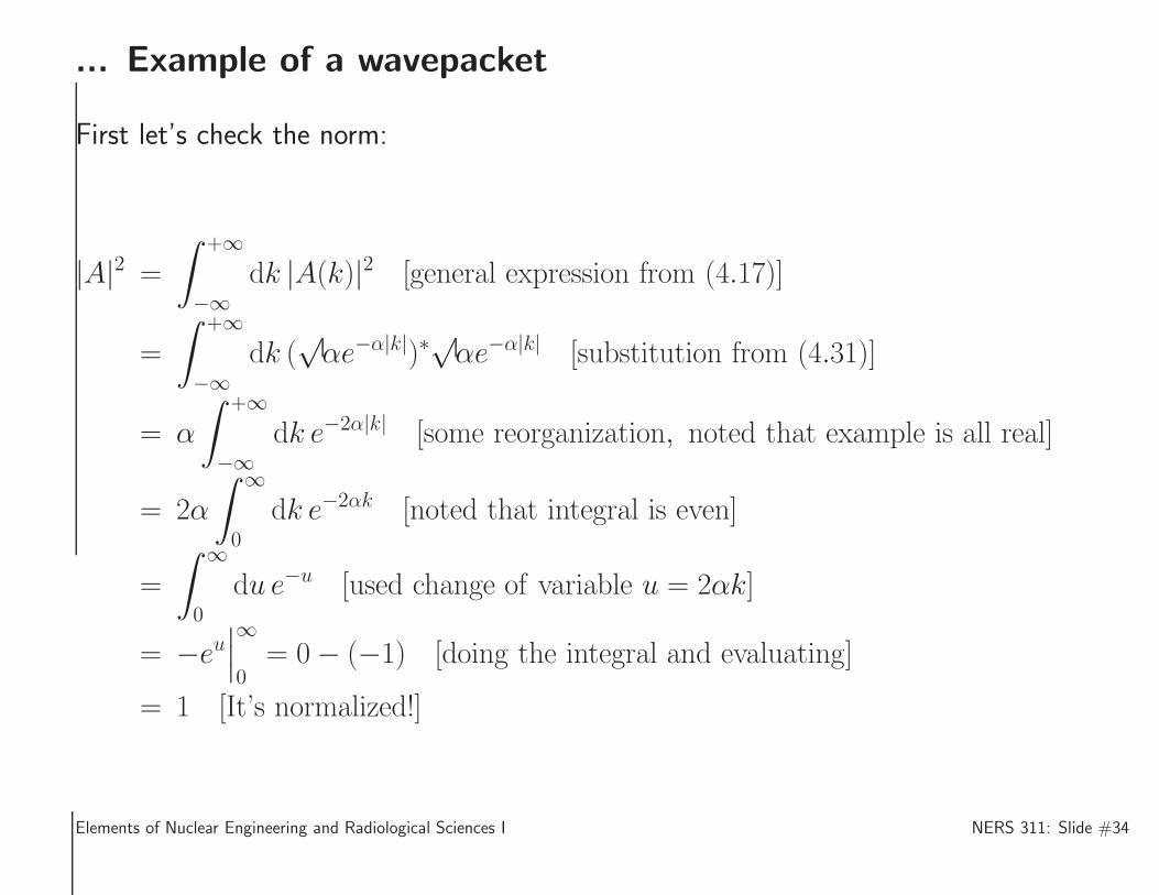
First let’s check the norm:
|A|2 =
∫ +∞
−∞dk |A(k)|2 [general expression from (4.17)]
=
∫ +∞
−∞dk (
√αe−α|k|)∗
√αe−α|k| [substitution from (4.31)]
= α
∫ +∞
−∞dk e−2α|k| [some reorganization, noted that example is all real]
= 2α
∫ ∞
0
dk e−2αk [noted that integral is even]
=
∫ ∞
0
du e−u [used change of variable u = 2αk]
= −eu∣
∣
∣
∞
0= 0− (−1) [doing the integral and evaluating]
= 1 [It’s normalized!]
Elements of Nuclear Engineering and Radiological Sciences I NERS 311: Slide #34
... Example of a wavepacket ...
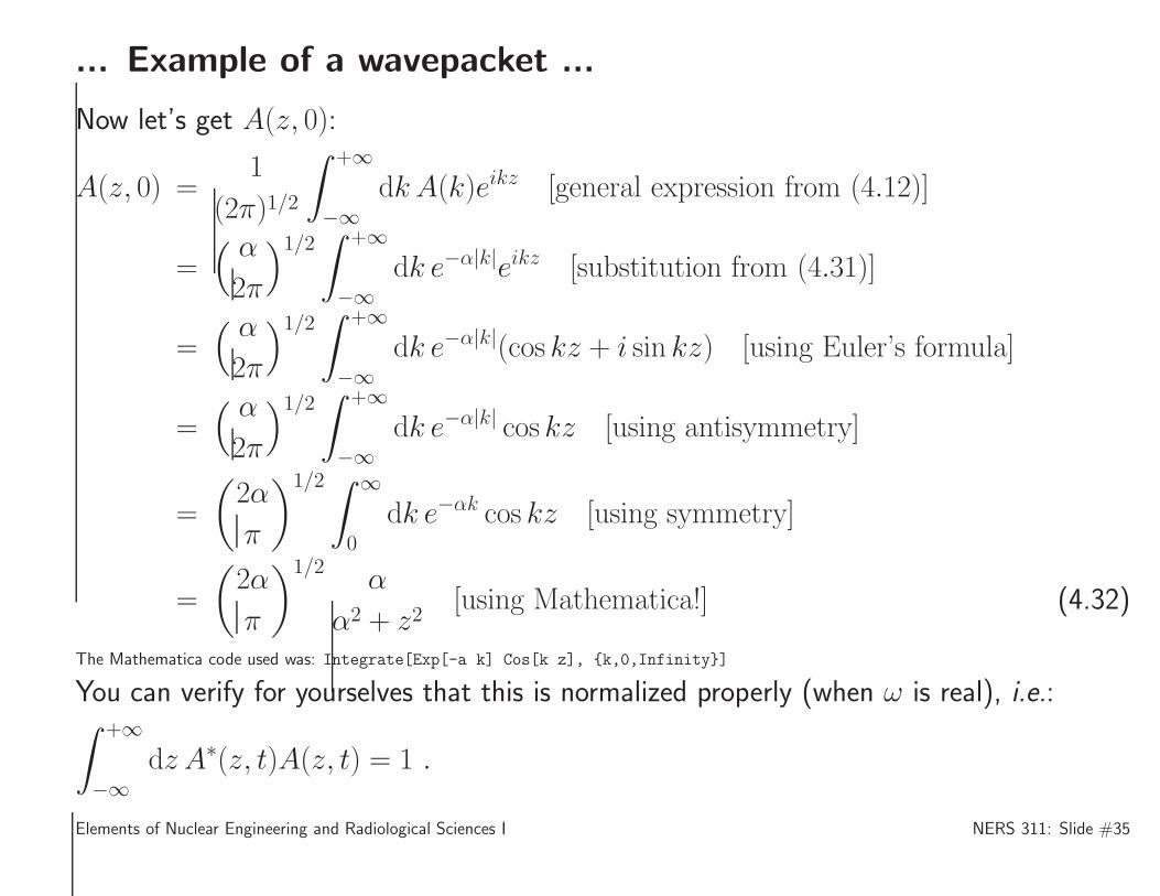
Now let’s get A(z, 0):
A(z, 0) =1
(2π)1/2
∫ +∞
−∞dk A(k)eikz [general expression from (4.12)]
=( α
2π
)1/2∫ +∞
−∞dk e−α|k|eikz [substitution from (4.31)]
=( α
2π
)1/2∫ +∞
−∞dk e−α|k|(cos kz + i sin kz) [using Euler’s formula]
=( α
2π
)1/2∫ +∞
−∞dk e−α|k| cos kz [using antisymmetry]
=
(
2α
π
)1/2 ∫ ∞
0
dk e−αk cos kz [using symmetry]
=
(
2α
π
)1/2α
α2 + z2[using Mathematica!] (4.32)
The Mathematica code used was: Integrate[Exp[-a k] Cos[k z], {k,0,Infinity}]
You can verify for yourselves that this is normalized properly (when ω is real), i.e.:∫ +∞
−∞dz A∗(z, t)A(z, t) = 1 .
Elements of Nuclear Engineering and Radiological Sciences I NERS 311: Slide #35
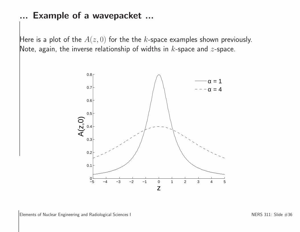
... Example of a wavepacket ...
Here is a plot of the A(z, 0) for the the k-space examples shown previously.Note, again, the inverse relationship of widths in k-space and z-space.
−5 −4 −3 −2 −1 0 1 2 3 4 50
0.1
0.2
0.3
0.4
0.5
0.6
0.7
0.8
z
A(z
,0)
α = 1α = 4
Elements of Nuclear Engineering and Radiological Sciences I NERS 311: Slide #36
... Example of a wavepacket ...
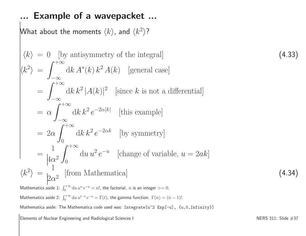
What about the moments 〈k〉, and 〈k2〉?
〈k〉 = 0 [by antisymmetry of the integral] (4.33)
〈k2〉 =
∫ +∞
−∞dk A∗(k) k2A(k) [general case]
=
∫ +∞
−∞dk k2 |A(k)|2 [since k is not a differential]
= α
∫ +∞
−∞dk k2 e−2α|k| [this example]
= 2α
∫ +∞
0
dk k2 e−2αk [by symmetry]
=1
4α2
∫ +∞
0
du u2 e−u [change of variable, u = 2ak]
〈k2〉 =1
2α2[from Mathematica] (4.34)
Mathematics aside 1:∫
+∞
0du un e−u = n!, the factorial. n is an integer >= 0.
Mathematics aside 2:∫
+∞
0du ut−1 e−u = Γ(t), the gamma function. Γ(n) = (n− 1)!.
Mathematica aside: The Mathematica code used was: Integrate[u^2 Exp[-u], {u,0,Infinity}]
Elements of Nuclear Engineering and Radiological Sciences I NERS 311: Slide #37
... Example of a wavepacket ...
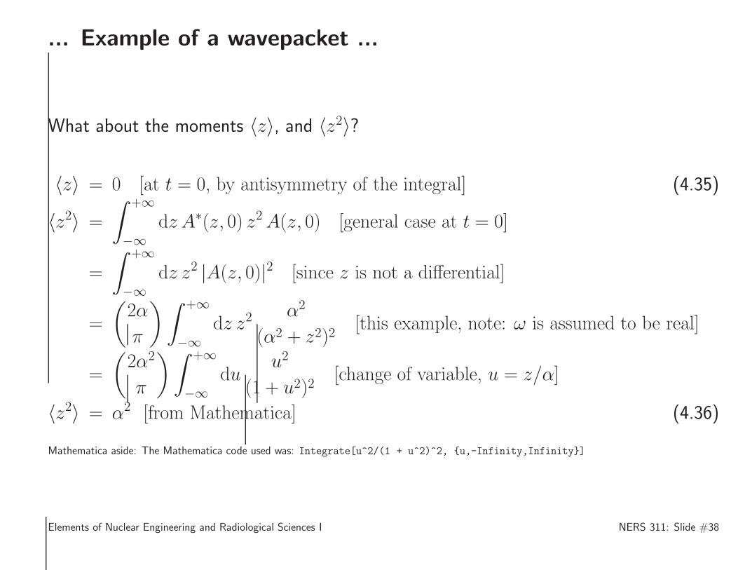
What about the moments 〈z〉, and 〈z2〉?
〈z〉 = 0 [at t = 0, by antisymmetry of the integral] (4.35)
〈z2〉 =
∫ +∞
−∞dz A∗(z, 0) z2A(z, 0) [general case at t = 0]
=
∫ +∞
−∞dz z2 |A(z, 0)|2 [since z is not a differential]
=
(
2α
π
)∫ +∞
−∞dz z2
α2
(α2 + z2)2[this example, note: ω is assumed to be real]
=
(
2α2
π
)∫ +∞
−∞du
u2
(1 + u2)2[change of variable, u = z/α]
〈z2〉 = α2 [from Mathematica] (4.36)
Mathematica aside: The Mathematica code used was: Integrate[u^2/(1 + u^2)^2, {u,-Infinity,Infinity}]
Elements of Nuclear Engineering and Radiological Sciences I NERS 311: Slide #38
... Example of a wavepacket ...
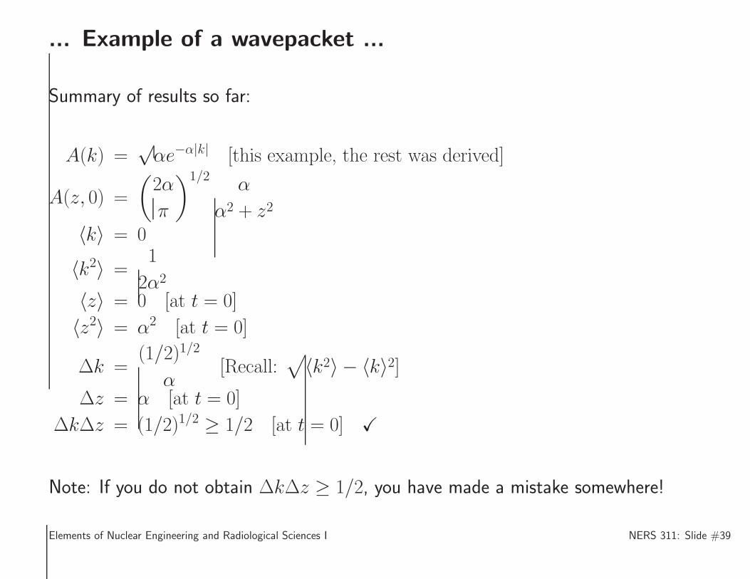
Summary of results so far:
A(k) =√αe−α|k| [this example, the rest was derived]
A(z, 0) =
(
2α
π
)1/2α
α2 + z2
〈k〉 = 0
〈k2〉 =1
2α2
〈z〉 = 0 [at t = 0]
〈z2〉 = α2 [at t = 0]
∆k =(1/2)1/2
α[Recall:
√
〈k2〉 − 〈k〉2]∆z = α [at t = 0]
∆k∆z = (1/2)1/2 ≥ 1/2 [at t = 0] X
Note: If you do not obtain ∆k∆z ≥ 1/2, you have made a mistake somewhere!
Elements of Nuclear Engineering and Radiological Sciences I NERS 311: Slide #39
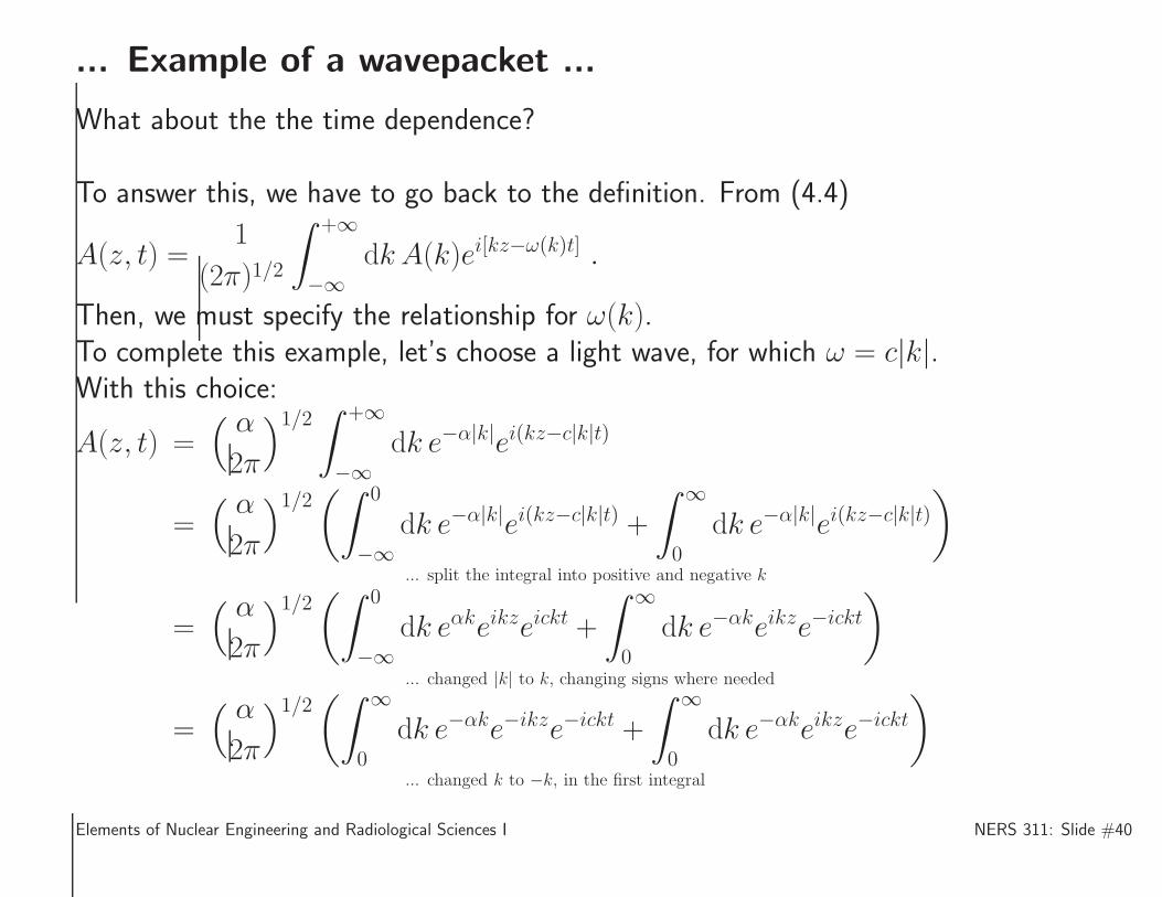
... Example of a wavepacket ...
What about the the time dependence?
To answer this, we have to go back to the definition. From (4.4)
A(z, t) =1
(2π)1/2
∫ +∞
−∞dk A(k)ei[kz−ω(k)t] .
Then, we must specify the relationship for ω(k).To complete this example, let’s choose a light wave, for which ω = c|k|.With this choice:
A(z, t) =( α
2π
)1/2∫ +∞
−∞dk e−α|k|ei(kz−c|k|t)
=( α
2π
)1/2(∫ 0
−∞dk e−α|k|ei(kz−c|k|t) +
∫ ∞
0
dk e−α|k|ei(kz−c|k|t))
... split the integral into positive and negative k
=( α
2π
)1/2(∫ 0
−∞dk eαkeikzeickt +
∫ ∞
0
dk e−αkeikze−ickt
)
... changed |k| to k, changing signs where needed
=( α
2π
)1/2(∫ ∞
0
dk e−αke−ikze−ickt +
∫ ∞
0
dk e−αkeikze−ickt
)
... changed k to −k, in the first integral
Elements of Nuclear Engineering and Radiological Sciences I NERS 311: Slide #40
... Example of a wavepacket ...
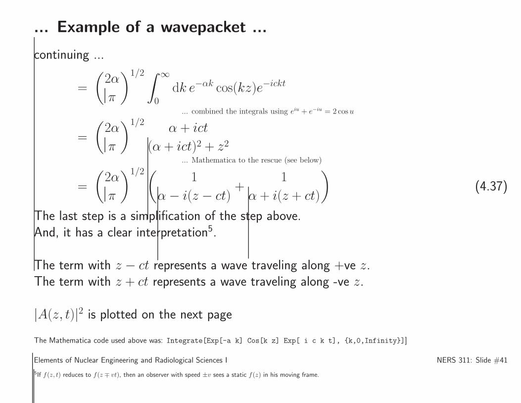
continuing ...
=
(
2α
π
)1/2 ∫ ∞
0
dk e−αk cos(kz)e−ickt
... combined the integrals using eiu + e−iu = 2 cosu
=
(
2α
π
)1/2α + ict
(α + ict)2 + z2... Mathematica to the rescue (see below)
=
(
2α
π
)1/2(1
α− i(z − ct)+
1
α + i(z + ct)
)
(4.37)
The last step is a simplification of the step above.And, it has a clear interpretation5.
The term with z − ct represents a wave traveling along +ve z.The term with z + ct represents a wave traveling along -ve z.
|A(z, t)|2 is plotted on the next page
The Mathematica code used above was: Integrate[Exp[-a k] Cos[k z] Exp[ i c k t], {k,0,Infinity}]]
Elements of Nuclear Engineering and Radiological Sciences I NERS 311: Slide #41
5If f(z, t) reduces to f(z ∓ vt), then an observer with speed ±v sees a static f(z) in his moving frame.
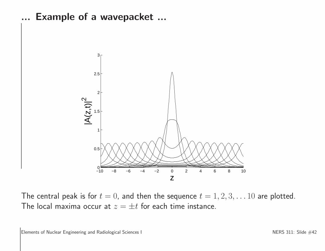
... Example of a wavepacket ...
−10 −8 −6 −4 −2 0 2 4 6 8 100
0.5
1
1.5
2
2.5
3
z
|A(z
,t)|2
The central peak is for t = 0, and then the sequence t = 1, 2, 3, . . . 10 are plotted.The local maxima occur at z = ±t for each time instance.
Elements of Nuclear Engineering and Radiological Sciences I NERS 311: Slide #42
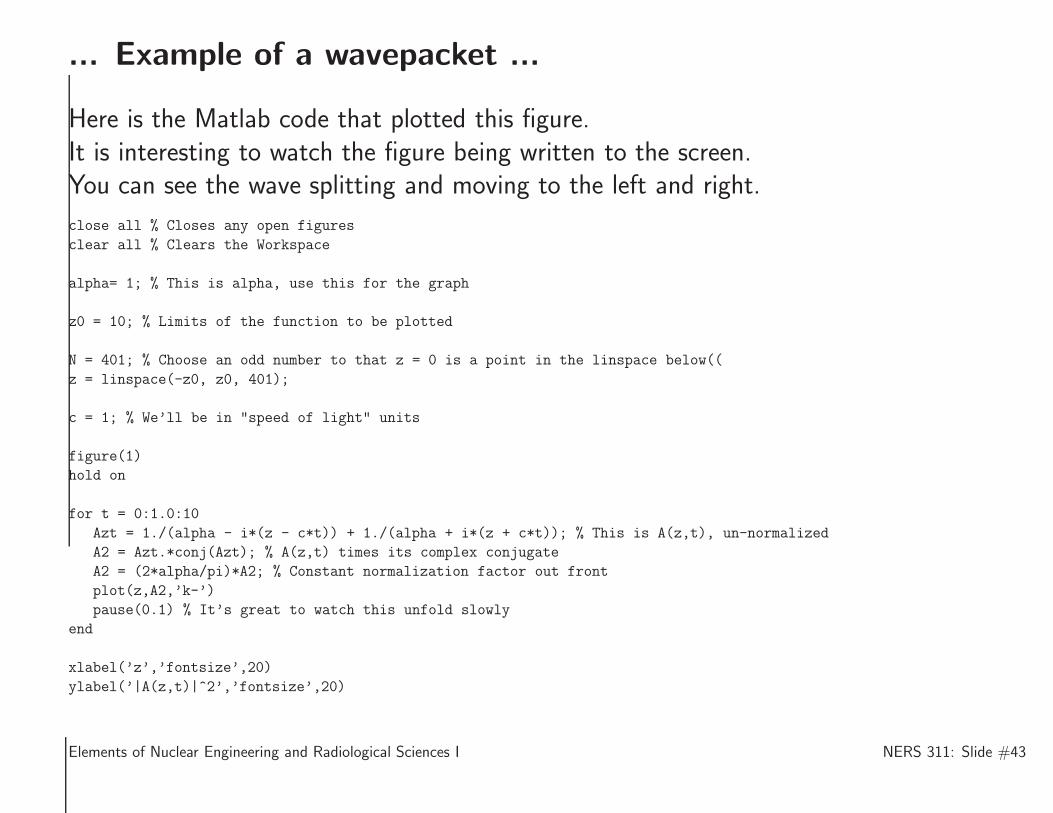
... Example of a wavepacket ...
Here is the Matlab code that plotted this figure.It is interesting to watch the figure being written to the screen.You can see the wave splitting and moving to the left and right.
close all % Closes any open figures
clear all % Clears the Workspace
alpha= 1; % This is alpha, use this for the graph
z0 = 10; % Limits of the function to be plotted
N = 401; % Choose an odd number to that z = 0 is a point in the linspace below((
z = linspace(-z0, z0, 401);
c = 1; % We’ll be in "speed of light" units
figure(1)
hold on
for t = 0:1.0:10
Azt = 1./(alpha - i*(z - c*t)) + 1./(alpha + i*(z + c*t)); % This is A(z,t), un-normalized
A2 = Azt.*conj(Azt); % A(z,t) times its complex conjugate
A2 = (2*alpha/pi)*A2; % Constant normalization factor out front
plot(z,A2,’k-’)
pause(0.1) % It’s great to watch this unfold slowly
end
xlabel(’z’,’fontsize’,20)
ylabel(’|A(z,t)|^2’,’fontsize’,20)
Elements of Nuclear Engineering and Radiological Sciences I NERS 311: Slide #43
Group velocity ...
Recall (4.4):
A(z, t) =1
(2π)1/2
∫ +∞
−∞dk A(k)ei[kz−ω(k)t] .
We have learned that this amplitude represents the kinematics of waves.Now, we want to draw a strong connection between the kinematics of waves (all of Chap-ter 4), to the kinematics of particles.
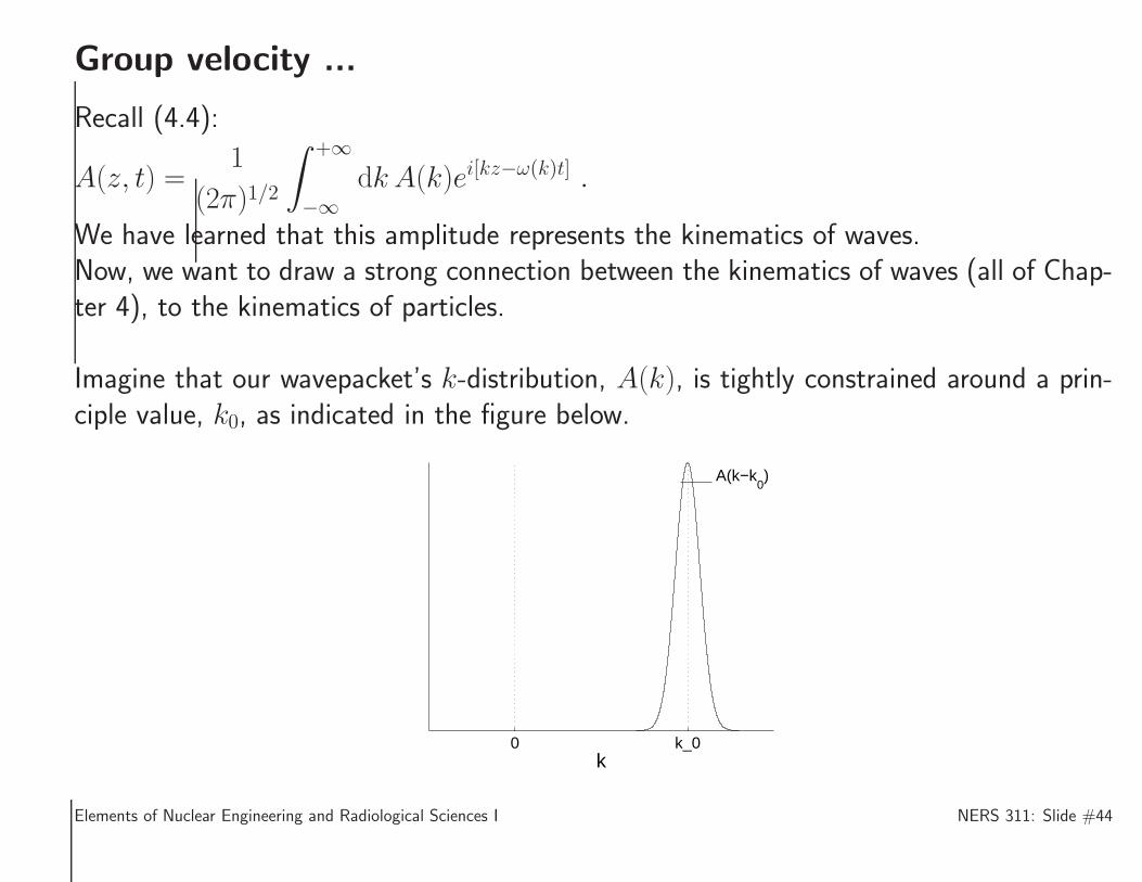
Imagine that our wavepacket’s k-distribution, A(k), is tightly constrained around a prin-ciple value, k0, as indicated in the figure below.
0 k_0k
A(k−k0)
Elements of Nuclear Engineering and Radiological Sciences I NERS 311: Slide #44
... Group velocity ...
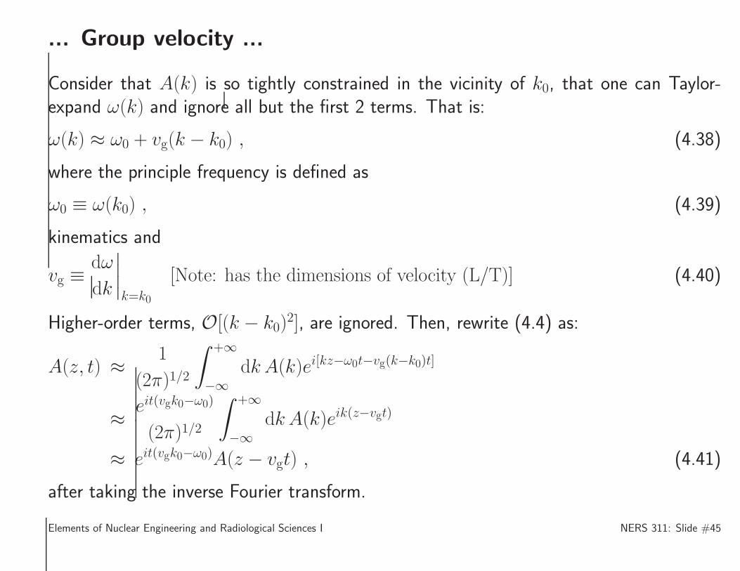
Consider that A(k) is so tightly constrained in the vicinity of k0, that one can Taylor-expand ω(k) and ignore all but the first 2 terms. That is:
ω(k) ≈ ω0 + vg(k − k0) , (4.38)
where the principle frequency is defined as
ω0 ≡ ω(k0) , (4.39)
kinematics and
vg ≡dω
dk
∣
∣
∣
∣
k=k0
[Note: has the dimensions of velocity (L/T)] (4.40)
Higher-order terms, O[(k − k0)2], are ignored. Then, rewrite (4.4) as:
A(z, t) ≈ 1
(2π)1/2
∫ +∞
−∞dk A(k)ei[kz−ω0t−vg(k−k0)t]
≈ eit(vgk0−ω0)
(2π)1/2
∫ +∞
−∞dk A(k)eik(z−vgt)
≈ eit(vgk0−ω0)A(z − vgt) , (4.41)
after taking the inverse Fourier transform.
Elements of Nuclear Engineering and Radiological Sciences I NERS 311: Slide #45
... Group velocity ...
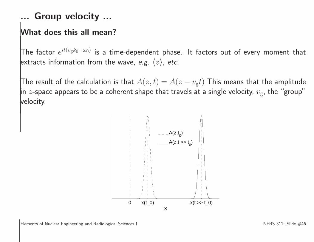
What does this all mean?
The factor eit(vgk0−ω0) is a time-dependent phase. It factors out of every moment thatextracts information from the wave, e.g. 〈z〉, etc.
The result of the calculation is that A(z, t) = A(z − vgt) This means that the amplitudein z-space appears to be a coherent shape that travels at a single velocity, vg, the “group”velocity.
0 x(t_0) x(t >> t_0)x
A(z,t0)
A(z,t >> t0)
Elements of Nuclear Engineering and Radiological Sciences I NERS 311: Slide #46
... Group velocity
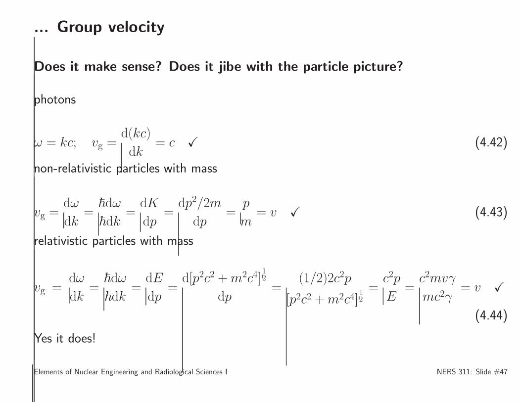
Does it make sense? Does it jibe with the particle picture?
photons
ω = kc; vg =d(kc)
dk= c X (4.42)
non-relativistic particles with mass
vg =dω
dk=
~dω
~dk=
dK
dp=
dp2/2m
dp=
p
m= v X (4.43)
relativistic particles with mass
vg =dω
dk=
~dω
~dk=
dE
dp=
d[p2c2 +m2c4]12
dp=
(1/2)2c2p
[p2c2 +m2c4]12
=c2p
E=
c2mvγ
mc2γ= v X
(4.44)
Yes it does!
Elements of Nuclear Engineering and Radiological Sciences I NERS 311: Slide #47

![Acceptance Rates (1) (black) Linst-mat.utalca.cl/jornadasbioestadistica2011/doc...Monte Carlo Methods with R: Metropolis–Hastings Algorithms [160] Acceptance Rates Normals from Double](https://static.fdocument.org/doc/165x107/6147bd3eafbe1968d37a3eb9/acceptance-rates-1-black-linst-mat-monte-carlo-methods-with-r-metropolisahastings.jpg)


![ORIGINAL ARTICLE Open Access β-Keto esters from ketones ...tory and antiphlogistic properties. Especially, a pyrazolone derivative (edaravone) [3] acts as a radical scavenger to interrupt](https://static.fdocument.org/doc/165x107/608fba6ac49a6d7592273fd2/original-article-open-access-keto-esters-from-ketones-tory-and-antiphlogistic.jpg)