4 - Mechanical Systems - University of Massachusetts Lowell
64
1 Dr. Peter Avitabile Modal Analysis & Controls Laboratory 22.451 Dynamic Systems – Chapter 4 Mechanical Systems Peter Avitabile Mechanical Engineering Department University of Massachusetts Lowell j ω σ UNSTABLE STABLE TIME FRF FRF TIME FRF TIME FRF TIME TIME TIME > 1.0 ζ = 1.0 ζ = 0.7 ζ = 0.3 ζ = 0.1 ζ = 0 ζ
Transcript of 4 - Mechanical Systems - University of Massachusetts Lowell
1 Dr. Peter AvitabileModal Analysis & Controls Laboratory22.451 Dynamic Systems – Chapter 4
Mechanical Systems
Peter AvitabileMechanical Engineering DepartmentUniversity of Massachusetts Lowell
jω
σ
UNSTABLESTABLE
TIME
FRF
FRF
TIME
FRF
TIME
FRF
TIME
TIME
TIME
> 1.0ζ
= 1.0ζ
= 0.7ζ
= 0.3ζ
= 0.1ζ = 0ζ
2 Dr. Peter AvitabileModal Analysis & Controls Laboratory22.451 Dynamic Systems – Chapter 4
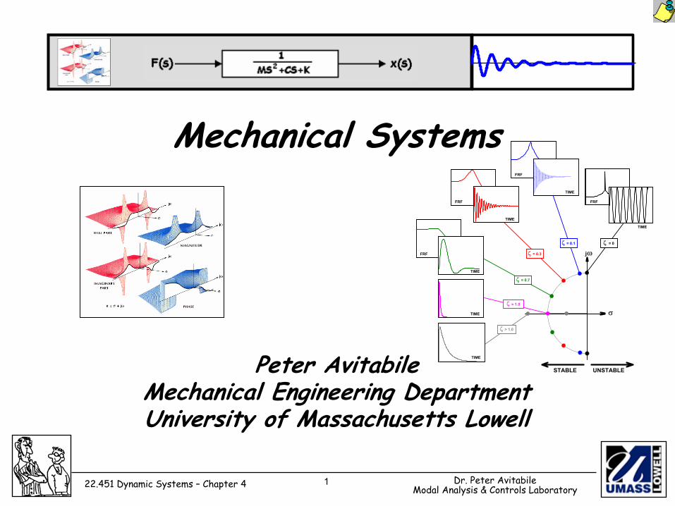
Mechanical Systems-Translational Mass Element
Translation of a particle moving in space due to an applied force is given by:
dtdpf =
Where:mvmomentump
forcef==
=
Considering the mass to be constant:
madtdvmfmdvfdt
dt)mv(df ==⇒=⇒=
3 Dr. Peter AvitabileModal Analysis & Controls Laboratory22.451 Dynamic Systems – Chapter 4
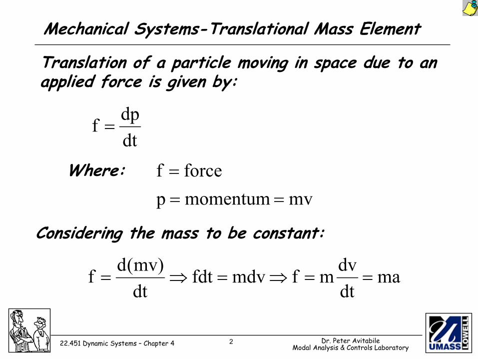
Mechanical Systems – Translational Mass Element
Displacement, velocity, and acceleration are all related by time derivatives as:
2
2
dtxd
dtda =ν
=
xva &&& ==
4 Dr. Peter AvitabileModal Analysis & Controls Laboratory22.451 Dynamic Systems – Chapter 4
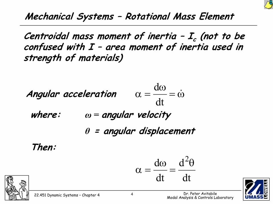
Mechanical Systems – Rotational Mass Element
ω=ω
=α &dtd
dtd
dtd 2θ
=ω
=α
Centroidal mass moment of inertia – Ic (not to be confused with I – area moment of inertia used in strength of materials)
Angular acceleration
where: ω = angular velocityθ = angular displacement
Then:
5 Dr. Peter AvitabileModal Analysis & Controls Laboratory22.451 Dynamic Systems – Chapter 4
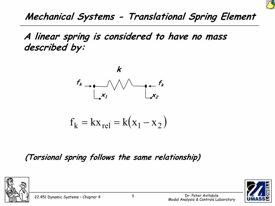
Mechanical Systems - Translational Spring Element
( )21relk xxkkxf −==
A linear spring is considered to have no mass described by:
(Torsional spring follows the same relationship)
fk fk
x1 x2
k
6 Dr. Peter AvitabileModal Analysis & Controls Laboratory22.451 Dynamic Systems – Chapter 4
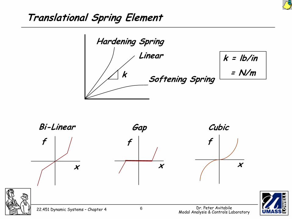
Translational Spring Element
Hardening Spring
Bi-Linear
Linear
Softening Spring
Gap Cubicf f f
x x x
k
k = lb/in= N/m
7 Dr. Peter AvitabileModal Analysis & Controls Laboratory22.451 Dynamic Systems – Chapter 4
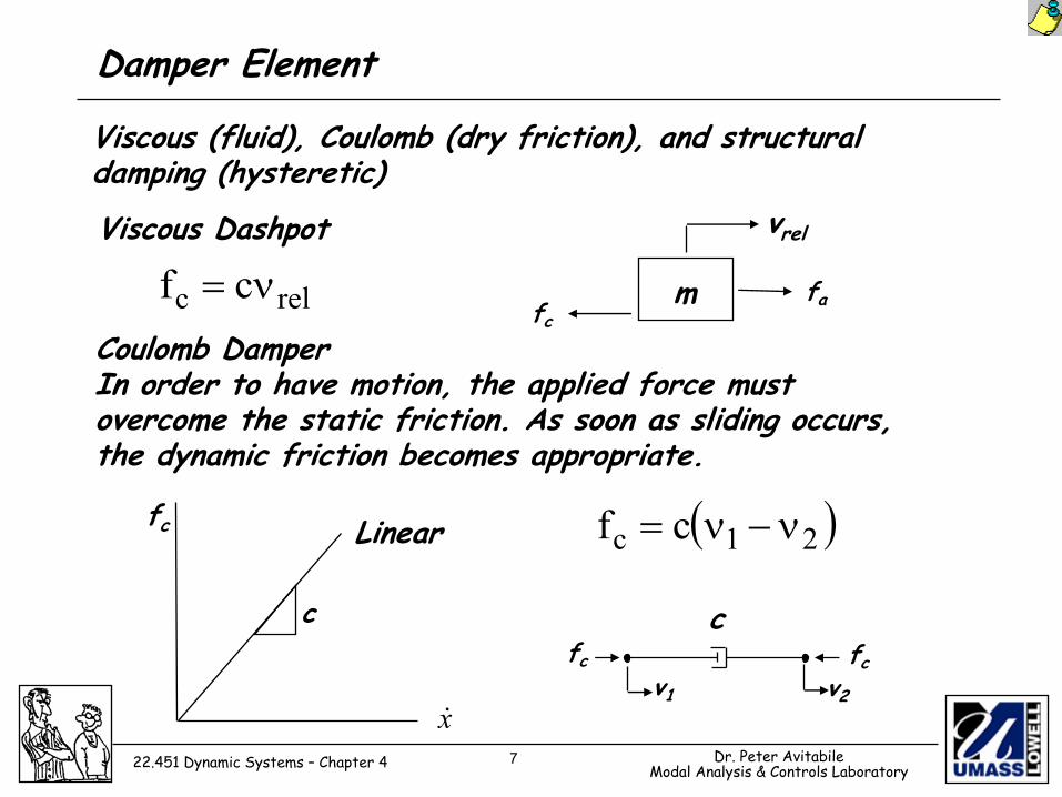
Damper Element
relc cf ν=
Viscous (fluid), Coulomb (dry friction), and structural damping (hysteretic)
Viscous Dashpot
fcfa
vrel
m
Coulomb DamperIn order to have motion, the applied force must overcome the static friction. As soon as sliding occurs, the dynamic friction becomes appropriate.
fc
c
x&
Linear ( )21c cf ν−ν=
fc fcv1 v2
c
8 Dr. Peter AvitabileModal Analysis & Controls Laboratory22.451 Dynamic Systems – Chapter 4
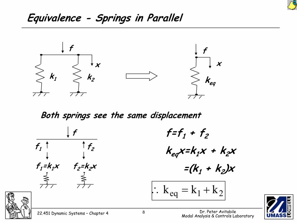
Equivalence - Springs in Parallel
Both springs see the same displacement
k2
x
f
k1
fx
keq
f2=k2x
f
f2
f1=k1x
f1
f=f1 + f2
keqx=k1x + k2x=(k1 + k2)x
21eq kkk +=∴
9 Dr. Peter AvitabileModal Analysis & Controls Laboratory22.451 Dynamic Systems – Chapter 4
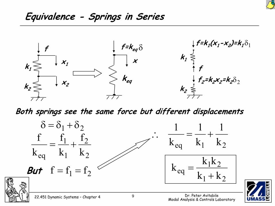
Equivalence - Springs in Series
Both springs see the same force but different displacements
But
∴
k2
x1
f
k1
x2
f=keq
x
keq
δ f=k1(x1-x2)=k1
k1
k2
f2=k2x2=k2
1δ
2δf
21 δ+δ=δ
2
2
1
1
eq kf
kf
kf
+= 21eq k1
k1
k1
+=
21
21eq kk
kkk+
=21 fff ==
10 Dr. Peter AvitabileModal Analysis & Controls Laboratory22.451 Dynamic Systems – Chapter 4
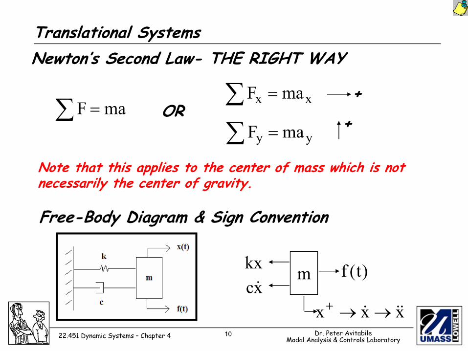
Translational SystemsNewton’s Second Law- THE RIGHT WAY
∑ = maF OR∑ = xx maF +
∑ = yy maF +
Note that this applies to the center of mass which is not necessarily the center of gravity.
Free-Body Diagram & Sign Convention
kxxc&
m )t(f
xxx &&& →→+
11 Dr. Peter AvitabileModal Analysis & Controls Laboratory22.451 Dynamic Systems – Chapter 4
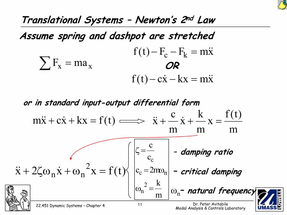
Translational Systems – Newton’s 2nd LawAssume spring and dashpot are stretched
∑ = xx maF
or in standard input-output differential form
xmFF)t(f kc &&=−−
xmkxxc)t(f &&& =−−OR
)t(fkxxcxm =++ &&&m)t(fx
mkx
mcx =++ &&&
)t(fxx2x 2nn =ω+ζω+ &&&
mkm2ccc
2n
nc
c
=ω
ω=
=ζ - damping ratio
– critical damping
ωn– natural frequency
12 Dr. Peter AvitabileModal Analysis & Controls Laboratory22.451 Dynamic Systems – Chapter 4
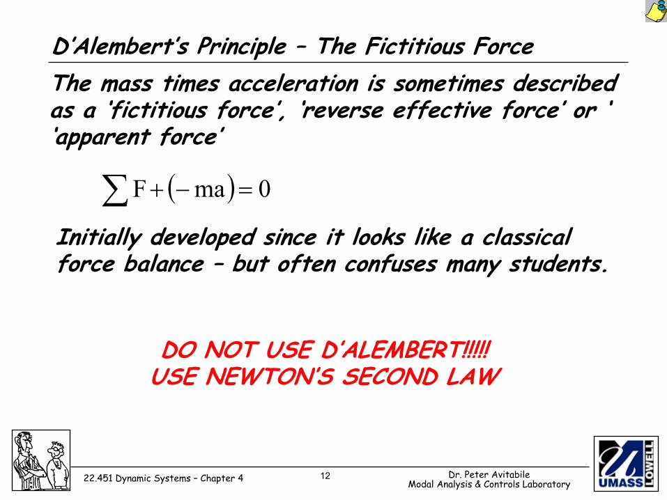
D’Alembert’s Principle – The Fictitious ForceThe mass times acceleration is sometimes describedas a ‘fictitious force’, ‘reverse effective force’ or ‘‘apparent force’
( )∑ =−+ 0maF
Initially developed since it looks like a classical force balance – but often confuses many students.
DO NOT USE D’ALEMBERT!!!!!USE NEWTON’S SECOND LAW
13 Dr. Peter AvitabileModal Analysis & Controls Laboratory22.451 Dynamic Systems – Chapter 4
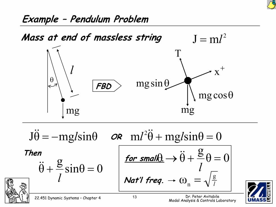
Example – Pendulum Problem
Mass at end of massless string
l
mg
θ
2mJ l=
+x
θcosmgmg
θsinmg
T
FBD
sinθmgθJ l−=&& 0sinθmgθm 2 =+ ll &&OR
Then
0sinθgθ =+l
&&0θgθθ =+→
l&&for small .
Nat’l freq. lg
nω =
14 Dr. Peter AvitabileModal Analysis & Controls Laboratory22.451 Dynamic Systems – Chapter 4
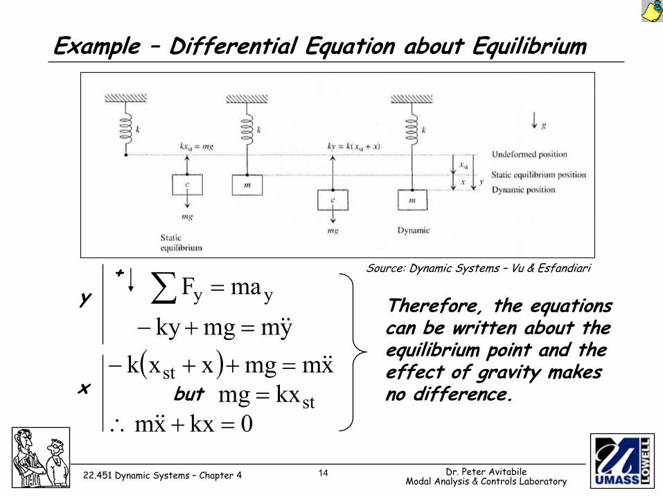
Example – Differential Equation about Equilibrium
y
x
+ ∑ = yy maFymmgky &&=+−
( ) xmmgxxk st &&=++−but stkxmg =
0kxxm =+∴ &&
Therefore, the equations can be written about the equilibrium point and the effect of gravity makes no difference.
Source: Dynamic Systems – Vu & Esfandiari
15 Dr. Peter AvitabileModal Analysis & Controls Laboratory22.451 Dynamic Systems – Chapter 4
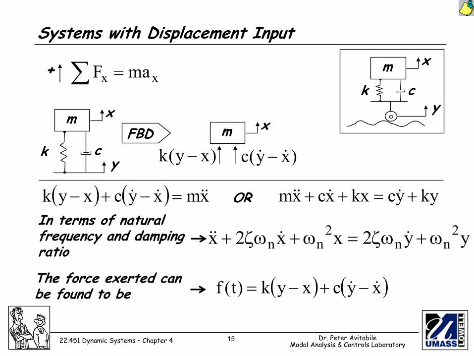
Systems with Displacement Input
In terms of natural frequency and damping ratio
∑ = xx maF+
m
ck
x
y
m x
)xy(c && −)xy(k −
mck
x
y
FBD
( ) ( ) xmxycxyk &&&& =−+− kyyckxxcxm +=++ &&&&OR
The force exerted can be found to be
yy2xx2x 2nn
2nn ω+ζω=ω+ζω+ &&&&
( ) ( )xycxyk)t(f && −+−=
16 Dr. Peter AvitabileModal Analysis & Controls Laboratory22.451 Dynamic Systems – Chapter 4
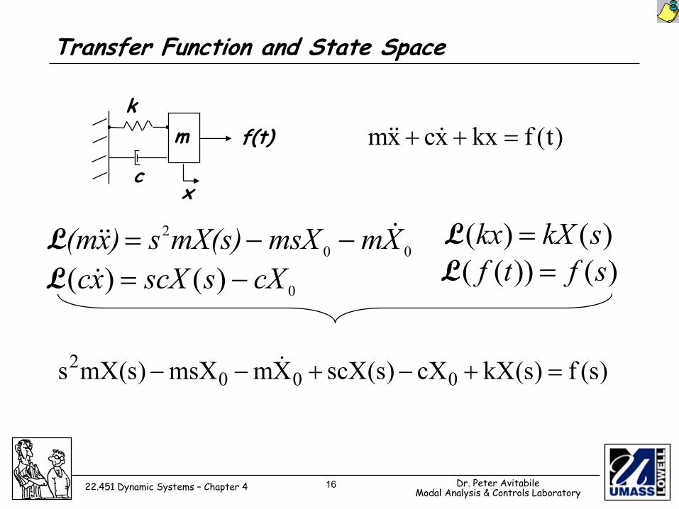
Transfer Function and State Space
m
c
k
x
f(t) )t(fkxxcxm =++ &&&
002 XmmsXmX(s)s)x(m &&& −−=L
0)()( cXsscXxc −=&L)()( skXkx =L)())(( sftf =L
)s(f)s(kXcX)s(scXXmmsX)s(mXs 0002 =+−+−− &
17 Dr. Peter AvitabileModal Analysis & Controls Laboratory22.451 Dynamic Systems – Chapter 4
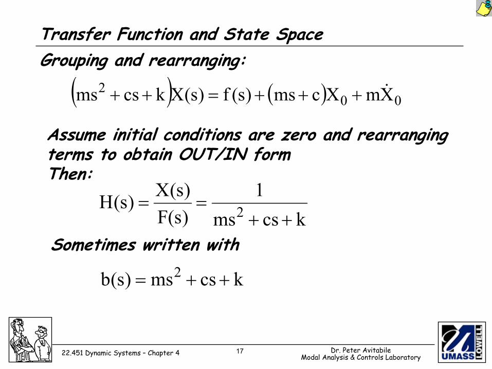
Transfer Function and State Space
( ) ( ) 002 XmXcms)s(f)s(Xkcsms &+++=++
Grouping and rearranging:
Assume initial conditions are zero and rearranging terms to obtain OUT/IN formThen:
kcsms1
)s(F)s(X)s(H 2 ++==
Sometimes written with
kcsms)s(b 2 ++=
18 Dr. Peter AvitabileModal Analysis & Controls Laboratory22.451 Dynamic Systems – Chapter 4
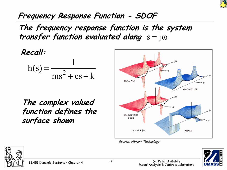
The frequency response function is the system transfer function evaluated along
Frequency Response Function - SDOF
ω= js
kcsms1)s(h 2 ++
=
Source: Vibrant Technology
Recall:
The complex valued function defines the surface shown
19 Dr. Peter AvitabileModal Analysis & Controls Laboratory22.451 Dynamic Systems – Chapter 4
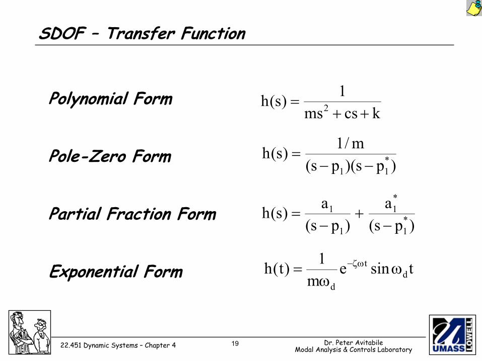
Polynomial Form
Pole-Zero Form
Partial Fraction Form
Exponential Form
kcsms1)s(h 2 ++
=
)ps)(ps(m/1)s(h *
11 −−=
)ps(a
)ps(a)s(h *
1
*1
1
1
−+
−=
tsinem1)t(h d
t
d
ωω
= ζω−
SDOF – Transfer Function
20 Dr. Peter AvitabileModal Analysis & Controls Laboratory22.451 Dynamic Systems – Chapter 4
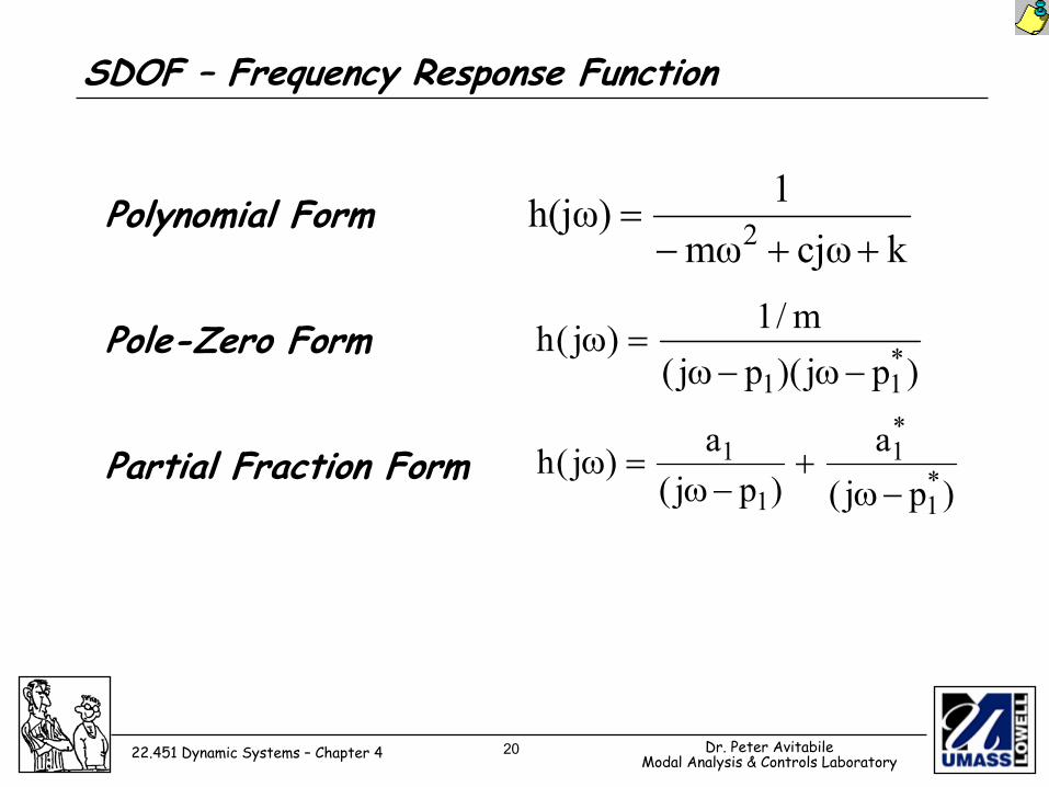
Polynomial Form
Pole-Zero Form
Partial Fraction Form
kcjωmω1)h(jω 2 ++−
=
)pj)(pj(m/1)j(h *
11 −ω−ω=ω
)pj(a
)pj(a)j(h *
1
*1
1
1
−ω+
−ω=ω
SDOF – Frequency Response Function
21 Dr. Peter AvitabileModal Analysis & Controls Laboratory22.451 Dynamic Systems – Chapter 4
Transfer Function approach is used extensively in design but is limited to linear, time-invariant systems.
SDOF – Transfer Function
1. T.F. – method to express output relative to input2. T.F. – system property – independent of the nature
of excitation3. T.F. contains necessary units but does not provide
physical structure of system4. If T.F. is known, then response can be evaluated
due to various inputs5. If T.F. is unknown, it can be established
experimentally by measuring output response due to known measured inputs
22 Dr. Peter AvitabileModal Analysis & Controls Laboratory22.451 Dynamic Systems – Chapter 4
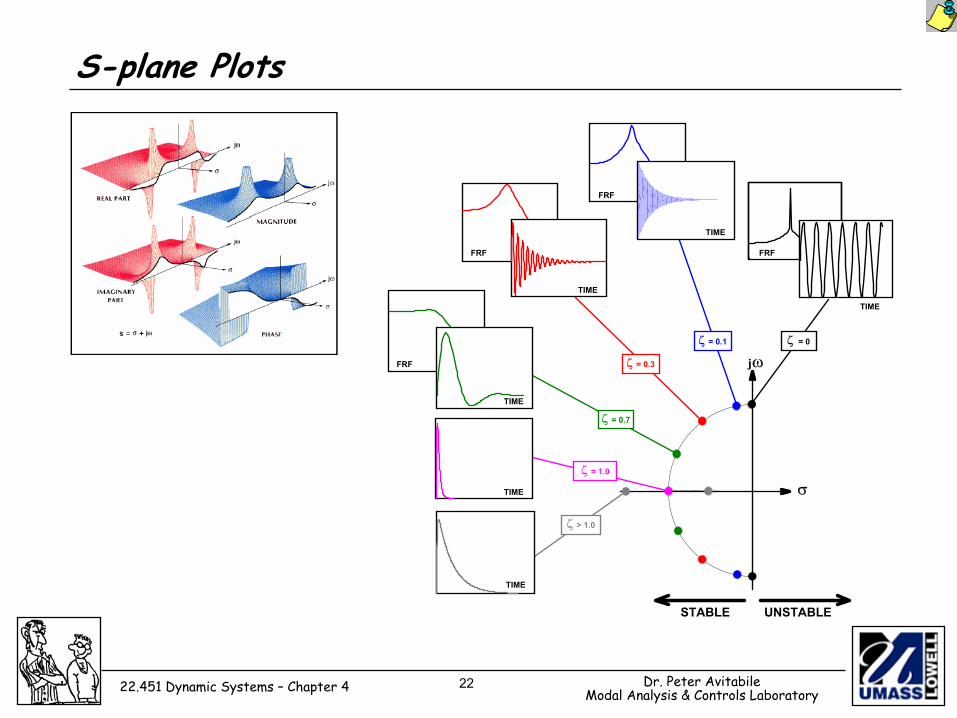
S-plane Plots
jω
σ
UNSTABLESTABLE
TIME
FRF
FRF
TIME
FRF
TIME
FRF
TIME
TIME
TIME
> 1.0ζ
= 1.0ζ
= 0.7ζ
= 0.3ζ
= 0.1ζ = 0ζ
23 Dr. Peter AvitabileModal Analysis & Controls Laboratory22.451 Dynamic Systems – Chapter 4
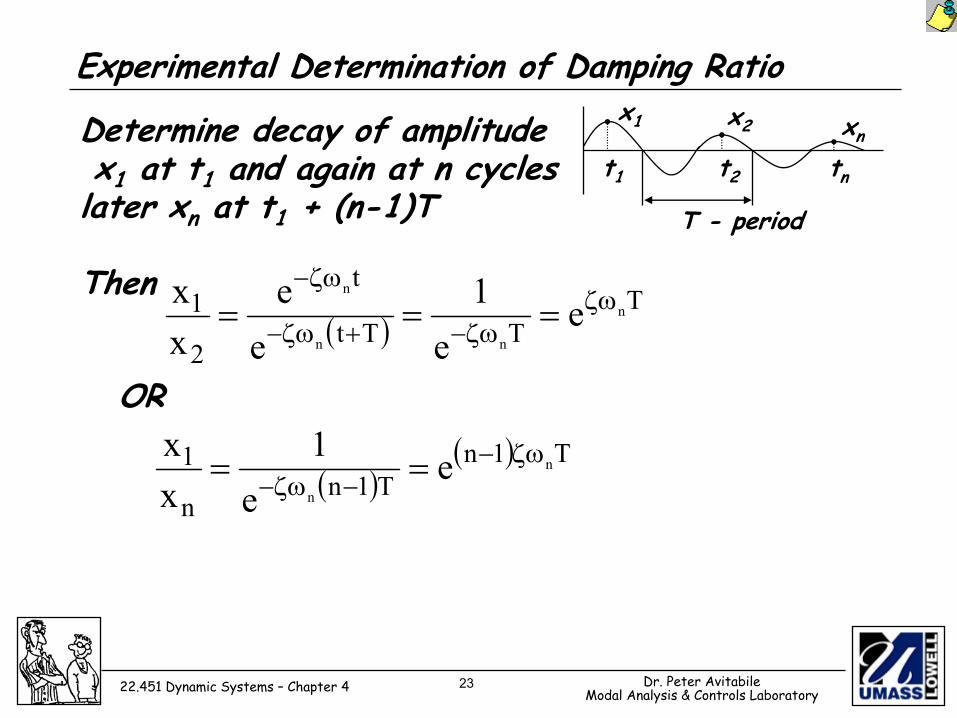
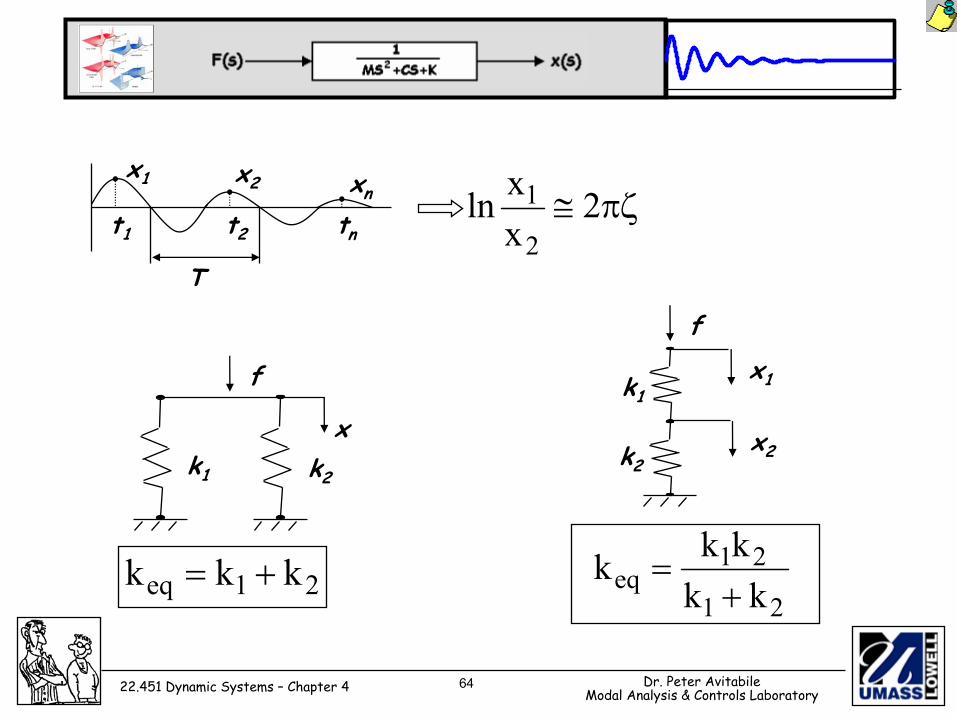
Experimental Determination of Damping Ratio
Determine decay of amplitudex1 at t1 and again at n cycleslater xn at t1 + (n-1)T
Then
x1 x2 xn
t1 t2 tn
T - period
( )T
TTt
t
2
1 n
nn
n
ee1
ee
xx ζω
ζω−+ζω−
ζω−===
OR
( )( ) T1n
T1nn
1 n
ne
e1
xx ζω−
−ζω− ==
24 Dr. Peter AvitabileModal Analysis & Controls Laboratory22.451 Dynamic Systems – Chapter 4
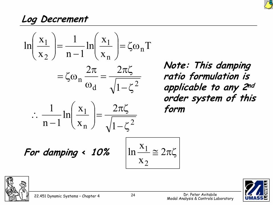
Log Decrement
Txxln
1n1
xxln n
n
1
2
1 ζω=
−
=
For damping < 10%
2dn
1
22
ζ−
πζ=
ωπ
ζω=
2n
1
1
2xxln
1n1
ζ−
πζ=
−
∴
πζ≅ 2xxln2
1
Note: This damping ratio formulation is applicable to any 2nd
order system of this form
25 Dr. Peter AvitabileModal Analysis & Controls Laboratory22.451 Dynamic Systems – Chapter 4
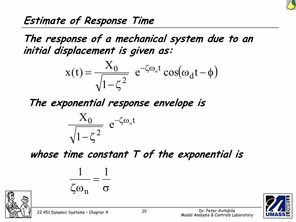
Estimate of Response Time
whose time constant T of the exponential is
( )φ−ωζ−
= ζω− tcose1
X)t(x dt
20 n
The response of a mechanical system due to an initial displacement is given as:
The exponential response envelope ist
20 ne
1
X ζω−
ζ−
σ=
ζω11
n
26 Dr. Peter AvitabileModal Analysis & Controls Laboratory22.451 Dynamic Systems – Chapter 4
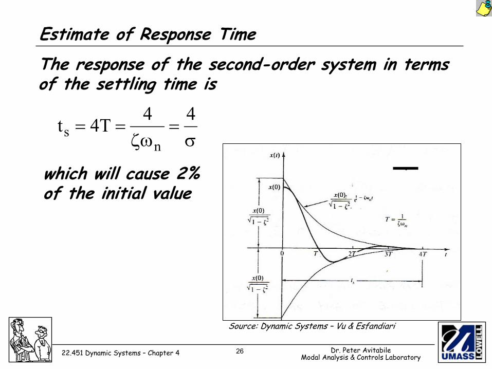
Estimate of Response TimeThe response of the second-order system in terms of the settling time is
σ=
ζω==
44T4tn
s
which will cause 2% of the initial value
Source: Dynamic Systems – Vu & Esfandiari

27 Dr. Peter AvitabileModal Analysis & Controls Laboratory22.451 Dynamic Systems – Chapter 4
State Space RepresentationThe ‘state’ of the system can be described in terms of the displacement and velocity as
=
xx
xx
2
1&
=
=)velocity(x)displ(x
xxX2
1&
u = f (force) and y = x (measured by sensor)
Then )t(fm1x
mcx
mkx +−−= &&&
OR
um1x
mcx
mkx 212 +−−=&
28 Dr. Peter AvitabileModal Analysis & Controls Laboratory22.451 Dynamic Systems – Chapter 4
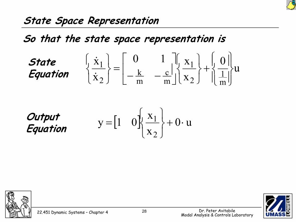
State Space RepresentationSo that the state space representation is
u0xx10
xx
m1
2
1
mc
mk
2
1
+
−−
=
&
&State Equation
Output Equation [ ] u0
xx01y2
1 ⋅+
=
29 Dr. Peter AvitabileModal Analysis & Controls Laboratory22.451 Dynamic Systems – Chapter 4
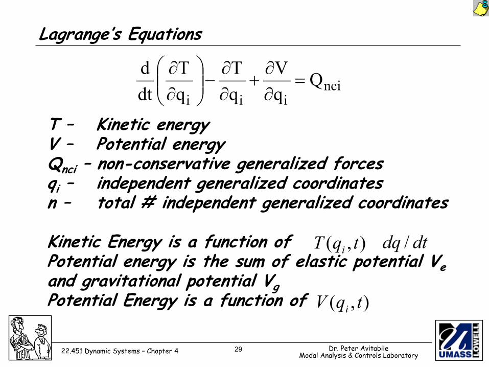
Lagrange’s Equations
nciiiiQ
qV
qT
qT
dtd
=∂∂
+∂∂
−
∂∂
T – Kinetic energyV – Potential energyQnci – non-conservative generalized forcesqi – independent generalized coordinatesn – total # independent generalized coordinates
Kinetic Energy is a function of Potential energy is the sum of elastic potential Veand gravitational potential VgPotential Energy is a function of
),( tqT i
),( tqV i
dtdq /
30 Dr. Peter AvitabileModal Analysis & Controls Laboratory22.451 Dynamic Systems – Chapter 4
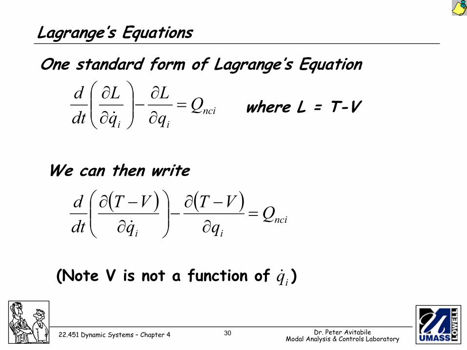
Lagrange’s Equations
nciii
QqL
qL
dtd
=∂∂
−
∂∂&
iq&
One standard form of Lagrange’s Equation
where L = T-V
We can then write
( ) ( )nci
ii
QqVT
qVT
dtd
=∂−∂
−
∂−∂&
(Note V is not a function of )
31 Dr. Peter AvitabileModal Analysis & Controls Laboratory22.451 Dynamic Systems – Chapter 4
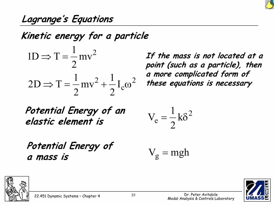
Lagrange’s Equations
2c
2
2
I21mv
21TD2
mv21TD1
ω+=⇒
=⇒
Kinetic energy for a particle
If the mass is not located at a point (such as a particle), then a more complicated form of these equations is necessary
Potential Energy of an elastic element is
Potential Energy of a mass is
2e k21V δ=
mghVg =
32 Dr. Peter AvitabileModal Analysis & Controls Laboratory22.451 Dynamic Systems – Chapter 4
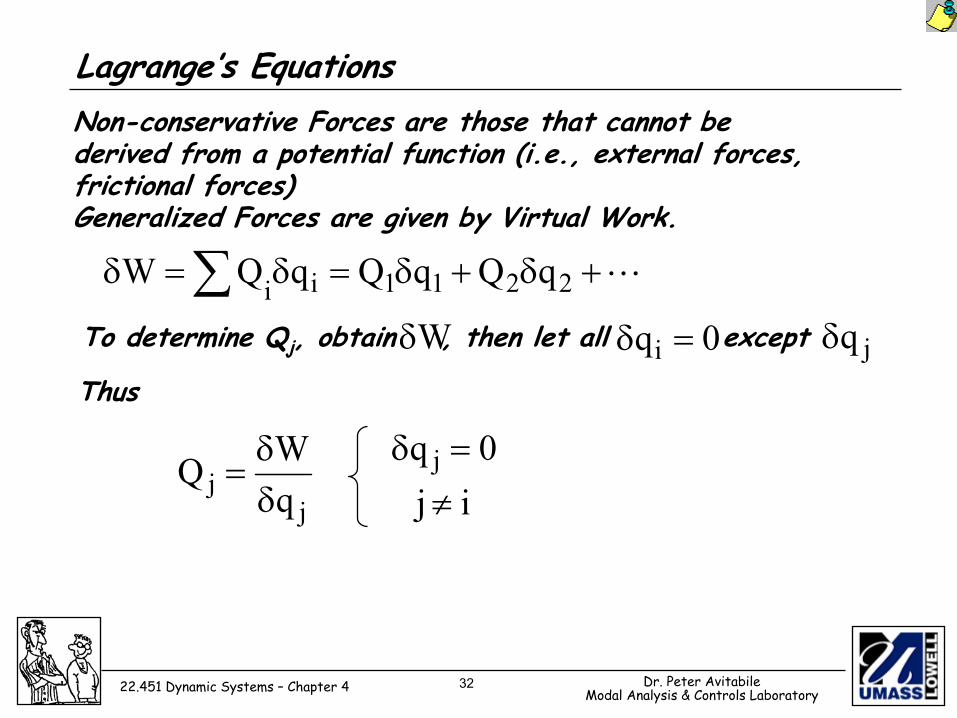
Lagrange’s EquationsNon-conservative Forces are those that cannot be derived from a potential function (i.e., external forces, frictional forces) Generalized Forces are given by Virtual Work.
To determine Qj, obtain , then let all except
L+δ+δ=δ=δ ∑ 2211ii qQqQqQW
Wδ 0qi =δ jqδThus
jj q
WQδδ
=0q j =δij ≠
33 Dr. Peter AvitabileModal Analysis & Controls Laboratory22.451 Dynamic Systems – Chapter 4
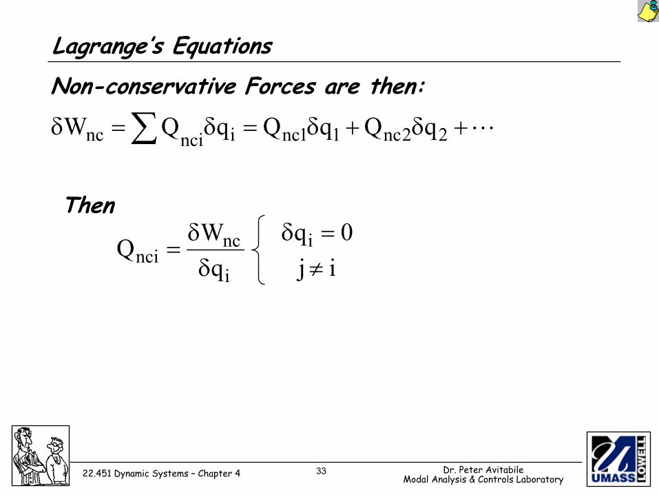
Lagrange’s EquationsNon-conservative Forces are then:
L+δ+δ=δ=δ ∑ 22nc11ncincinc qQqQqQW
Then
i
ncnci q
WQδδ
=0qi =δij ≠
34 Dr. Peter AvitabileModal Analysis & Controls Laboratory22.451 Dynamic Systems – Chapter 4
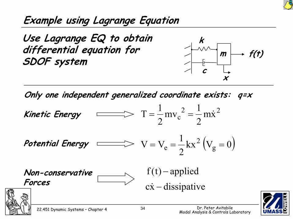
Example using Lagrange EquationUse Lagrange EQ to obtain differential equation for SDOF system
Only one independent generalized coordinate exists: q=x
22c xm
21mv
21T &==
m
c
k
x
f(t)
Kinetic Energy
Potential Energy
Non-conservative Forces
( )0Vkx21VV g
2e ===
applied)t(f −
edissipativxc −&
35 Dr. Peter AvitabileModal Analysis & Controls Laboratory22.451 Dynamic Systems – Chapter 4
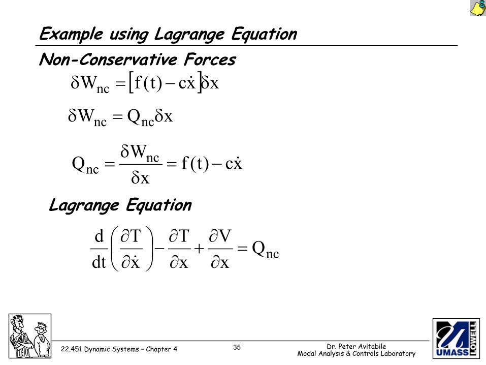
Example using Lagrange EquationNon-Conservative Forces
[ ] xxc)t(fWnc δ−=δ &
xQW ncnc δ=δ
xc)t(fxWQ nc
nc &−=δ
δ=
Lagrange Equation
ncQxV
xT
xT
dtd
=∂∂
+∂∂
−
∂∂&
36 Dr. Peter AvitabileModal Analysis & Controls Laboratory22.451 Dynamic Systems – Chapter 4
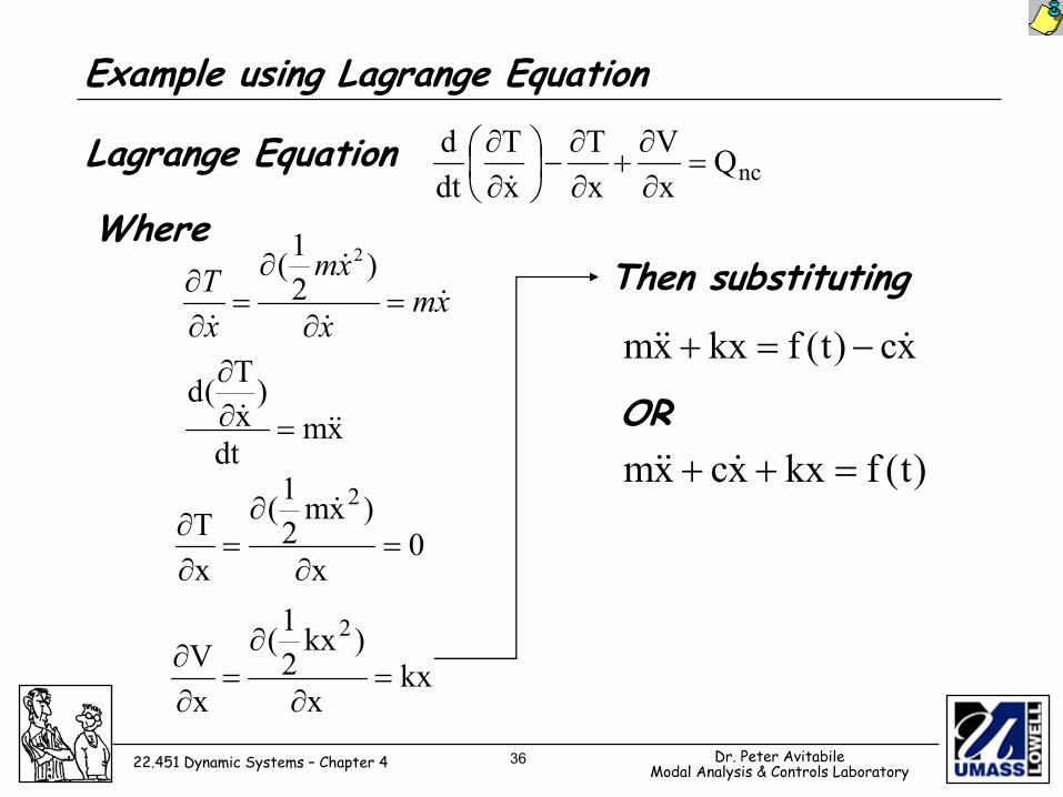
Example using Lagrange Equation
Lagrange Equation ncQxV
xT
xT
dtd
=∂∂
+∂∂
−
∂∂&
WhereThen substituting
xmx
xm
xT
&&
&
&=
∂
∂=
∂∂ )
21( 2
xmdt
)xT(d
&&& =∂∂
0x
)xm21(
xT
2
=∂
∂=
∂∂ &
kxx
)kx21(
xV
2
=∂
∂=
∂∂
OR
xc)t(fkxxm &&& −=+
)t(fkxxcxm =++ &&&
37 Dr. Peter AvitabileModal Analysis & Controls Laboratory22.451 Dynamic Systems – Chapter 4
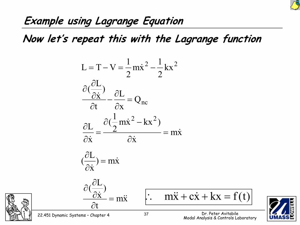
Example using Lagrange EquationNow let’s repeat this with the Lagrange function
22 kx21xm
21VTL −=−= &
xmt
)xL(
&&& =∂∂∂
∂
xmx
)kxxm21(
xL
22
&&
&
&=
∂
−∂=
∂∂
)t(fkxxcxm =++∴ &&&
ncQxL
t
)xL(
=∂∂
−∂∂∂
∂&
xm)xL( &&
=∂∂
38 Dr. Peter AvitabileModal Analysis & Controls Laboratory22.451 Dynamic Systems – Chapter 4
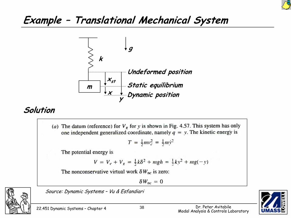
Example – Translational Mechanical System
m
k
xst
xy
g
Undeformed position
Dynamic positionStatic equilibrium
Solution
Source: Dynamic Systems – Vu & Esfandiari
39 Dr. Peter AvitabileModal Analysis & Controls Laboratory22.451 Dynamic Systems – Chapter 4
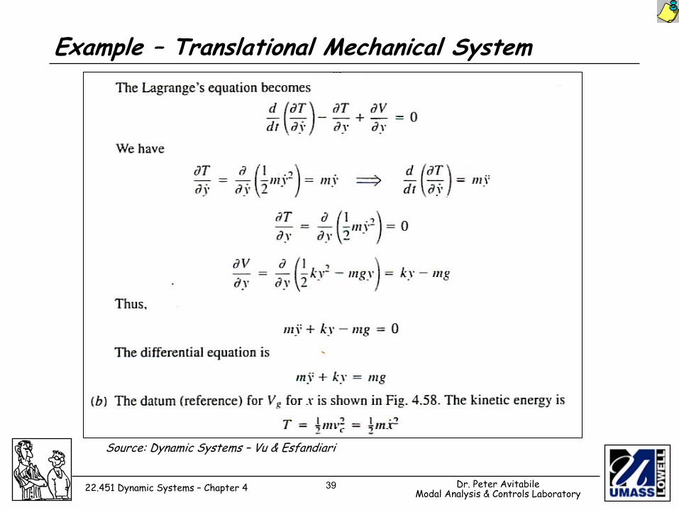
Example – Translational Mechanical System
Source: Dynamic Systems – Vu & Esfandiari
40 Dr. Peter AvitabileModal Analysis & Controls Laboratory22.451 Dynamic Systems – Chapter 4
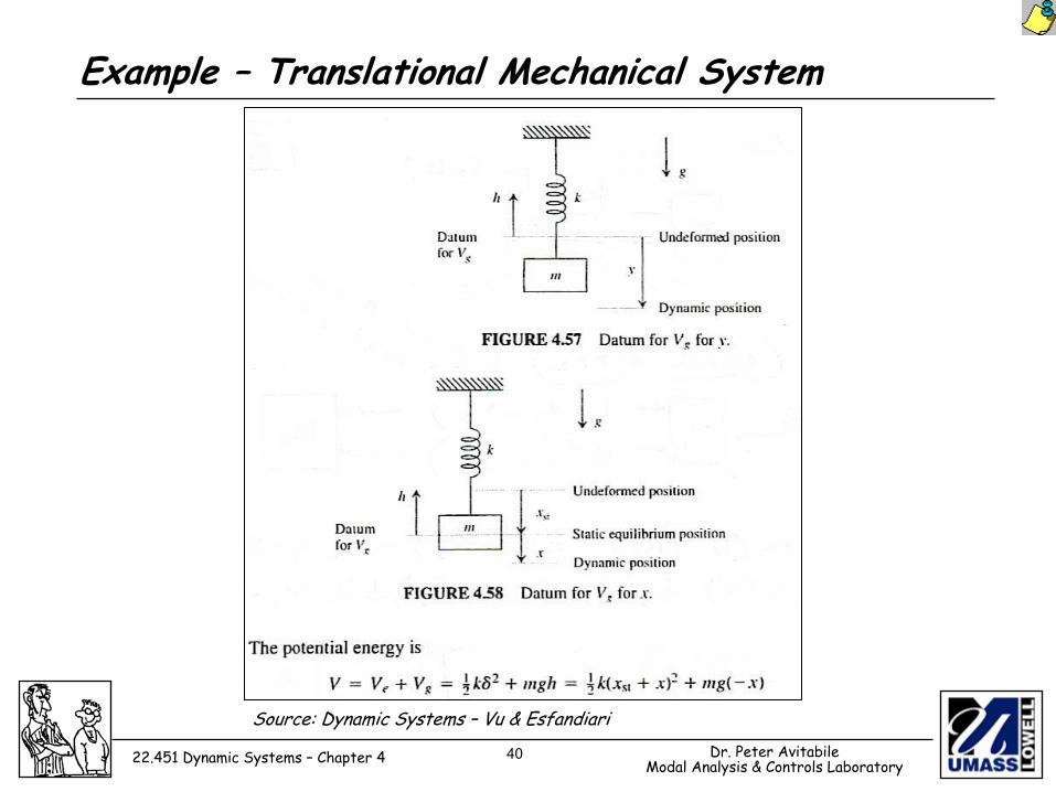
Example – Translational Mechanical System
Source: Dynamic Systems – Vu & Esfandiari
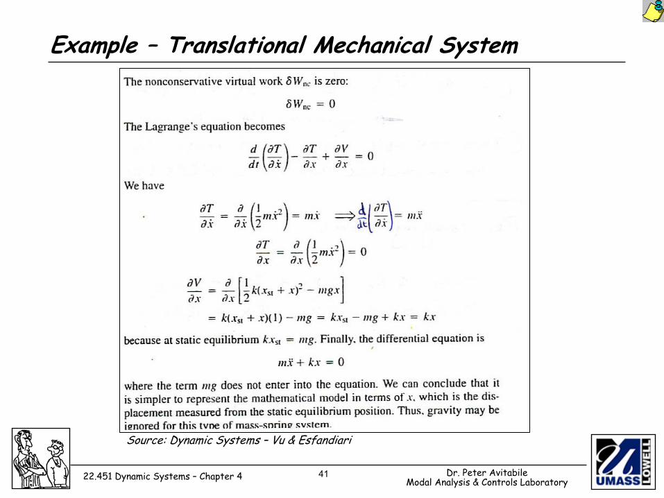
41 Dr. Peter AvitabileModal Analysis & Controls Laboratory22.451 Dynamic Systems – Chapter 4
Example – Translational Mechanical System
Source: Dynamic Systems – Vu & Esfandiari
42 Dr. Peter AvitabileModal Analysis & Controls Laboratory22.451 Dynamic Systems – Chapter 4
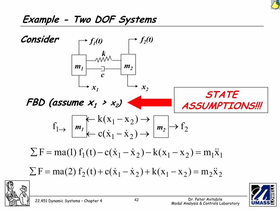
Example - Two DOF Systems
Consider
m1
f1(t)
x2x1
f2(t)
m2c
k
FBD (assume x1 > x2)
1121211 xm)xx(k)xx(c)t(f)1(maF &&&& =−−−−=∑
2221212 xm)xx(k)xx(c)t(f)2(maF &&&& =−+−+=∑
221
211 f
)xx(c)xx(k
f →→−←→−←
→ &&m2m1
STATE ASSUMPTIONS!!!
43 Dr. Peter AvitabileModal Analysis & Controls Laboratory22.451 Dynamic Systems – Chapter 4
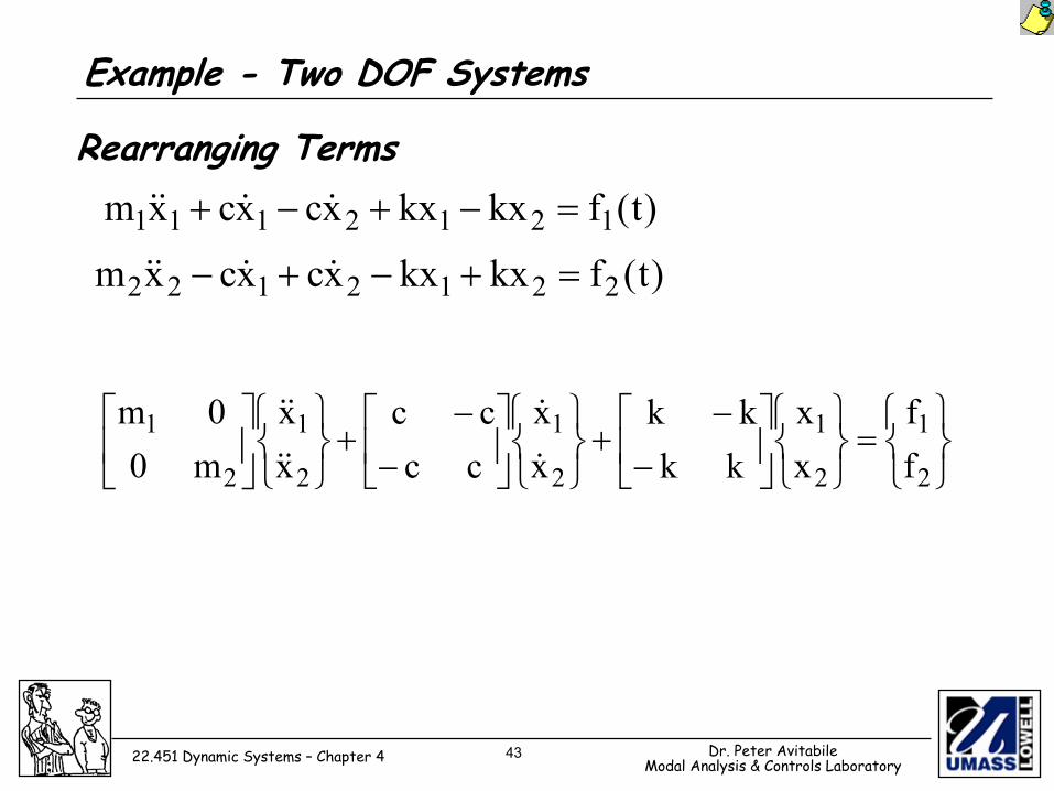
Example - Two DOF Systems
Rearranging Terms)t(fkxkxxcxcxm 1212111 =−+−+ &&&&
=
−
−+
−
−+
2
1
2
1
2
1
2
1
2
1
ff
xx
kkkk
xx
cccc
xx
m00m
&
&
&&
&&
)t(fkxkxxcxcxm 2212122 =+−+− &&&&
44 Dr. Peter AvitabileModal Analysis & Controls Laboratory22.451 Dynamic Systems – Chapter 4
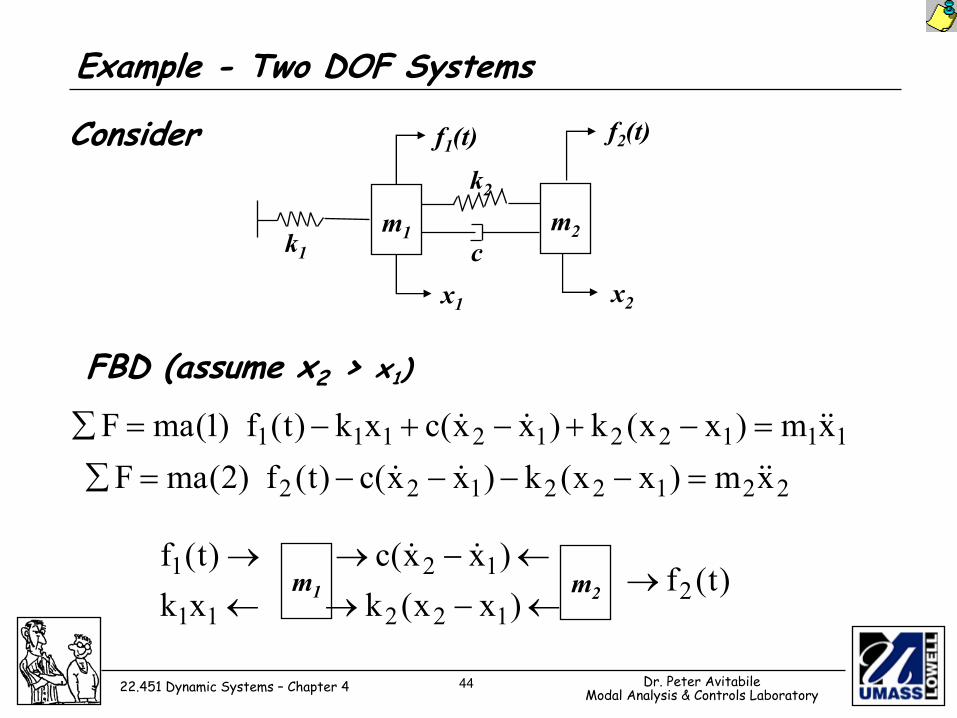
Example - Two DOF Systems
Consider
FBD (assume x2 > x1)
1112212111 xm)xx(k)xx(cxk)t(f)1(maF &&&& =−+−+−=∑
m1
f1(t)
x2x1
f2(t)
m2c
k2
k1
22122122 xm)xx(k)xx(c)t(f)2(maF &&&& =−−−−=∑
)t(f)xx(k)xx(c
xk)t(f
2122
12
11
1 →←−→←−→
←→ &&
m2m1
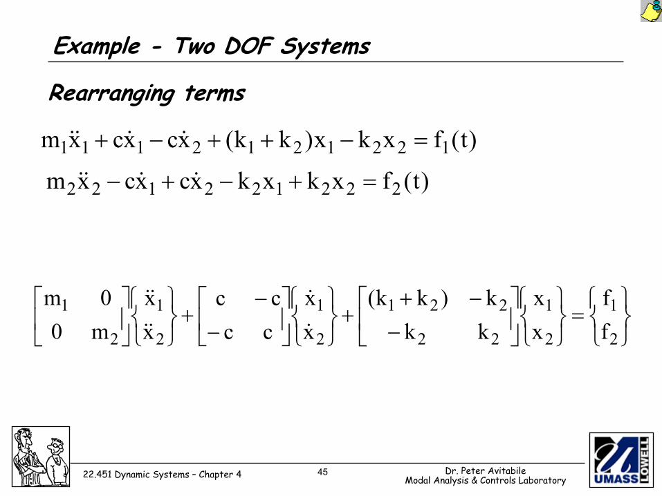
45 Dr. Peter AvitabileModal Analysis & Controls Laboratory22.451 Dynamic Systems – Chapter 4
Example - Two DOF Systems
Rearranging terms
)t(fxkx)kk(xcxcxm 1221212111 =−++−+ &&&&
=
−
−++
−
−+
2
1
2
1
22
221
2
1
2
1
2
1
ff
xx
kkk)kk(
xx
cccc
xx
m00m
&
&
&&
&&
)t(fxkxkxcxcxm 222122122 =+−+− &&&&
46 Dr. Peter AvitabileModal Analysis & Controls Laboratory22.451 Dynamic Systems – Chapter 4
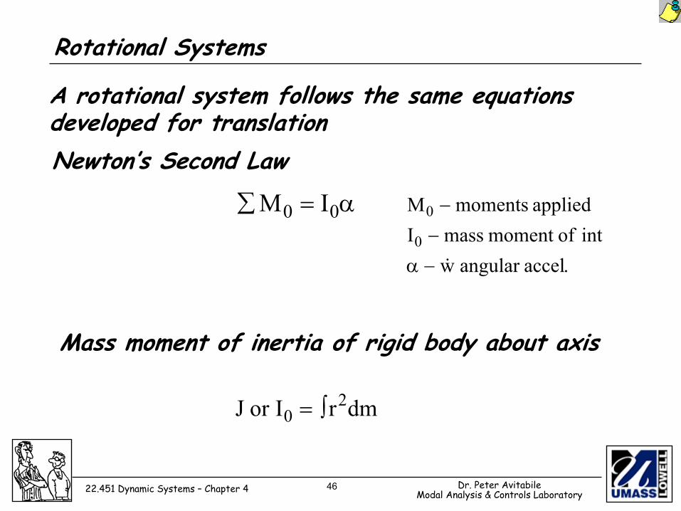
Rotational Systems
A rotational system follows the same equations developed for translation
α=∑ 00 IM
dmrIorJ 20 ∫=
Newton’s Second Law
.accelangularwintofmomentmassI
appliedmomentsM
0
0
&−α−−
Mass moment of inertia of rigid body about axis
47 Dr. Peter AvitabileModal Analysis & Controls Laboratory22.451 Dynamic Systems – Chapter 4
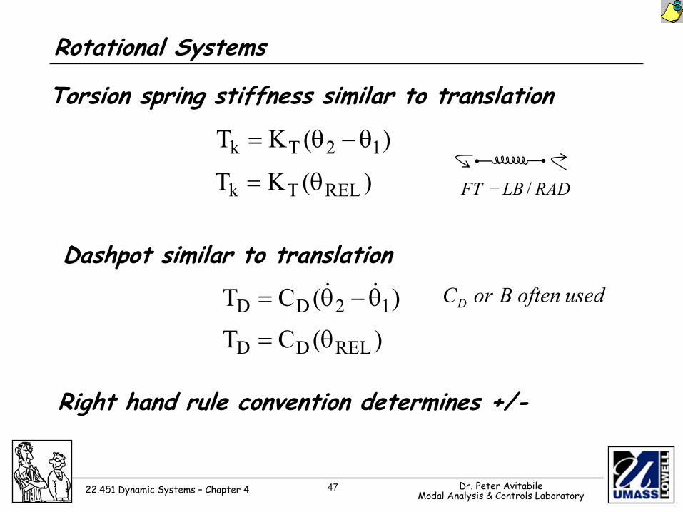
Rotational Systems
Torsion spring stiffness similar to translation
)(KT 12Tk θ−θ=
Dashpot similar to translation
Right hand rule convention determines +/-
)(KT RELTk θ=
)(CT 12DD θ−θ= &&
)(CT RELDD θ=
usedoftenBorCD
RADLBFT /−
48 Dr. Peter AvitabileModal Analysis & Controls Laboratory22.451 Dynamic Systems – Chapter 4
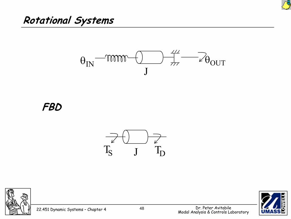
Rotational Systems
FBD
OUTθJ
INθ
J DTST
49 Dr. Peter AvitabileModal Analysis & Controls Laboratory22.451 Dynamic Systems – Chapter 4
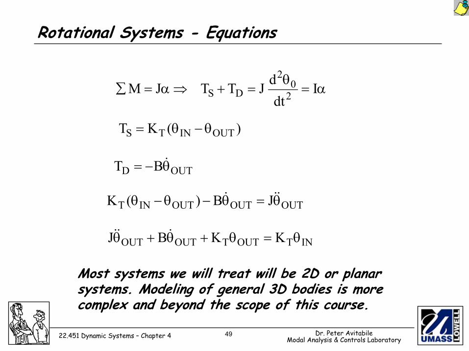
Rotational Systems - Equations
Most systems we will treat will be 2D or planar systems. Modeling of general 3D bodies is more complex and beyond the scope of this course.
α=θ
=+⇒α=∑ IdtdJTTJM 2
02
DS
)(KT OUTINTS θ−θ=
OUTD BT θ−= &
OUTOUTOUTINT JB)(K θ=θ−θ−θ &&&
INTOUTTOUTOUT KKBJ θ=θ+θ+θ &&&
50 Dr. Peter AvitabileModal Analysis & Controls Laboratory22.451 Dynamic Systems – Chapter 4
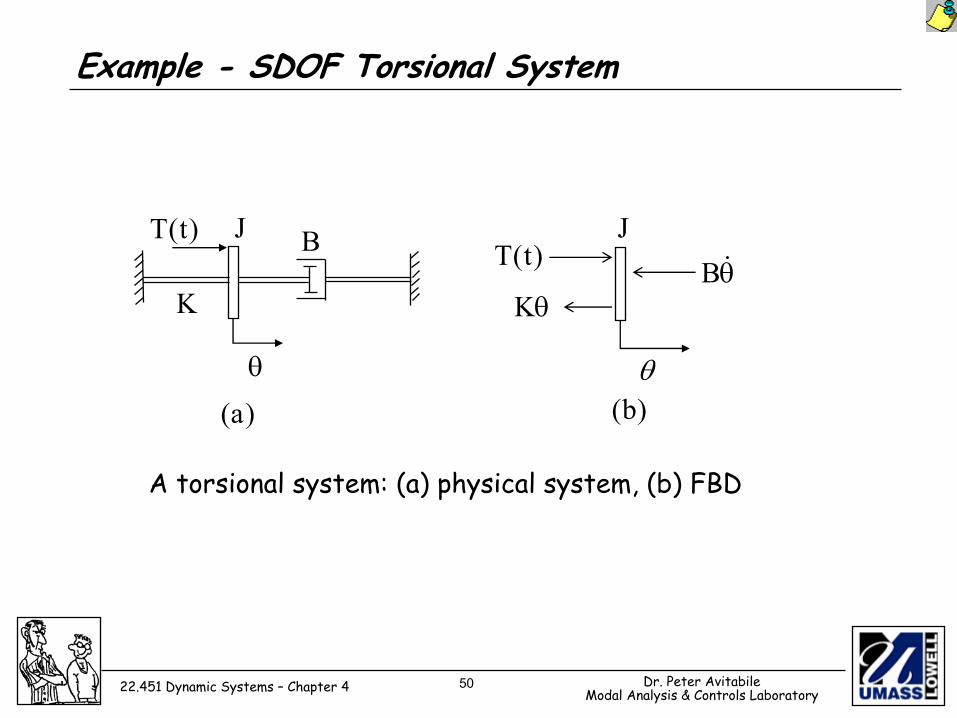
Example - SDOF Torsional System
A torsional system: (a) physical system, (b) FBD
θ&BθK
θ
)t(TJ
K
B
θ
)t(T J
)a( )b(
51 Dr. Peter AvitabileModal Analysis & Controls Laboratory22.451 Dynamic Systems – Chapter 4
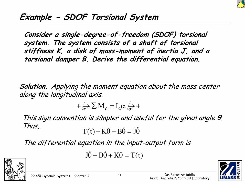
Example - SDOF Torsional System
This sign convention is simpler and useful for the given angle θ. Thus,
Consider a single-degree-of-freedom (SDOF) torsional system. The system consists of a shaft of torsional stiffness K, a disk of mass-moment of inertia J, and a torsional damper B. Derive the differential equation.
Solution. Applying the moment equation about the mass center along the longitudinal axis.
+→α=∑→+ cc IM
θ=θ−θ− &&& JBK)t(T
)t(TKBJ =θ+θ+θ &&&
The differential equation in the input-output form is
52 Dr. Peter AvitabileModal Analysis & Controls Laboratory22.451 Dynamic Systems – Chapter 4
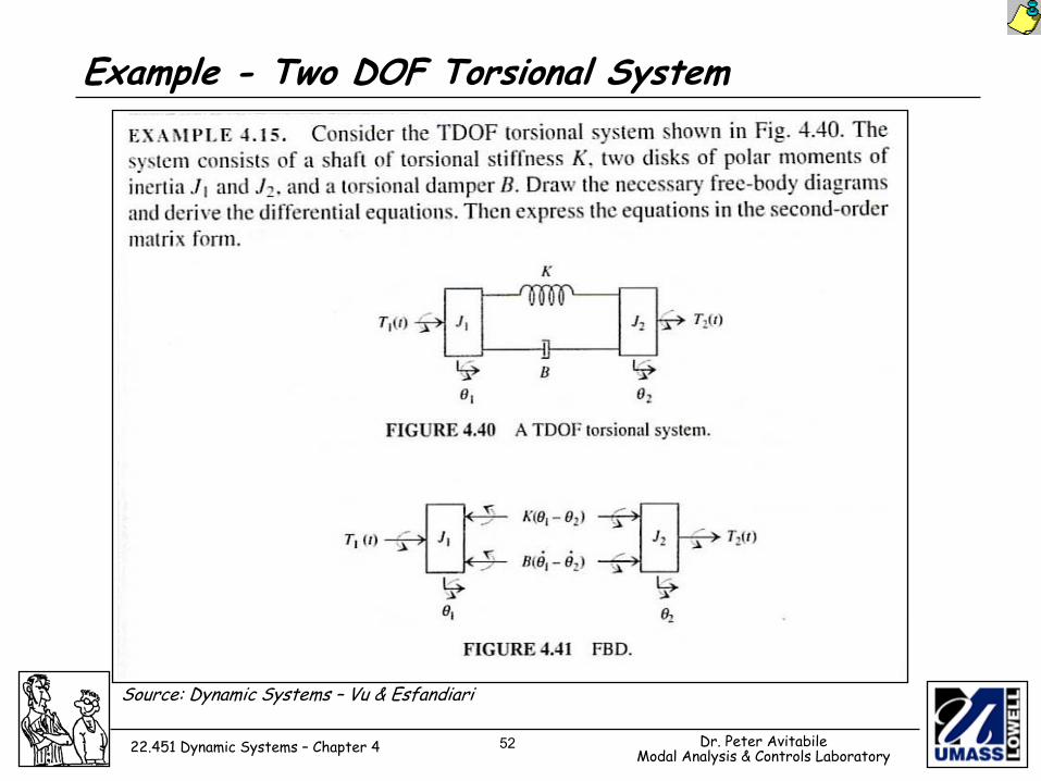
Example - Two DOF Torsional System
Source: Dynamic Systems – Vu & Esfandiari
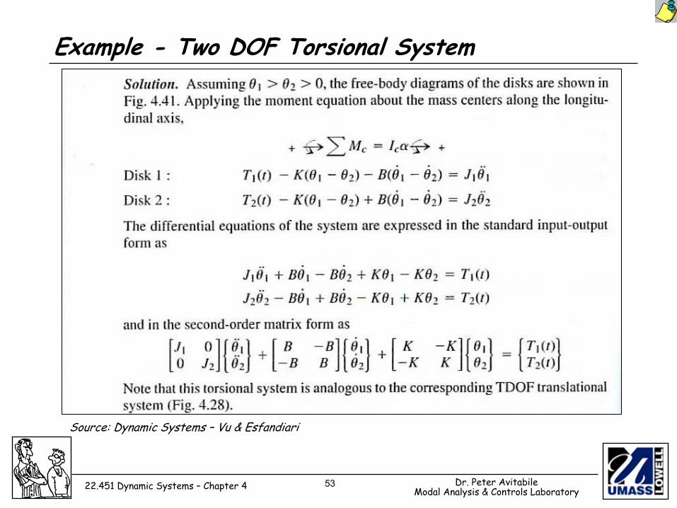
53 Dr. Peter AvitabileModal Analysis & Controls Laboratory22.451 Dynamic Systems – Chapter 4
Example - Two DOF Torsional System
Source: Dynamic Systems – Vu & Esfandiari
54 Dr. Peter AvitabileModal Analysis & Controls Laboratory22.451 Dynamic Systems – Chapter 4
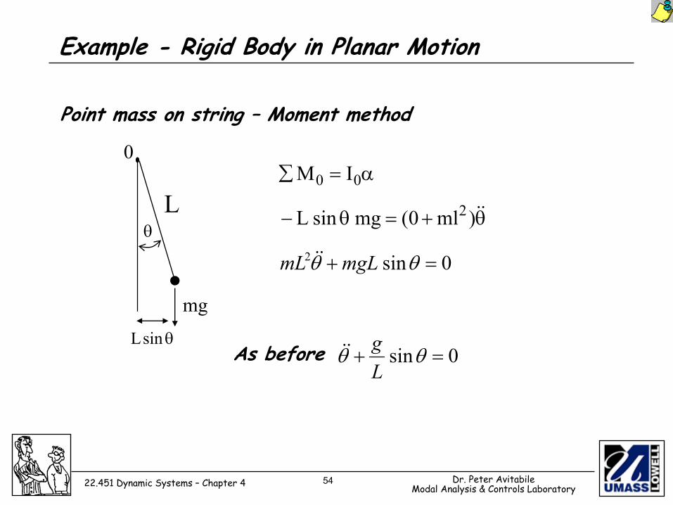
Example - Rigid Body in Planar Motion
As before
α=∑ 00 IM
θ+=θ− &&)ml0(mgsinL 2
Point mass on string – Moment method
0sin2 =+ θθ mgLmL &&
0sin =+ θθLg&&
L
mg
θ
0
θsinL
55 Dr. Peter AvitabileModal Analysis & Controls Laboratory22.451 Dynamic Systems – Chapter 4
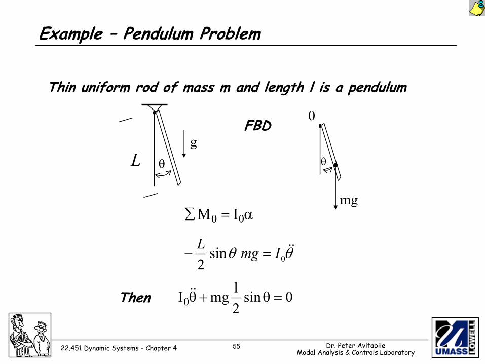
Example – Pendulum Problem
Thin uniform rod of mass m and length l is a pendulum
Then
α=∑ 00 IM
θθ &&0sin
2ImgL
=−
FBD
0sin2lmgI0 =θ+θ&&
0
mg
θLg
θ
56 Dr. Peter AvitabileModal Analysis & Controls Laboratory22.451 Dynamic Systems – Chapter 4
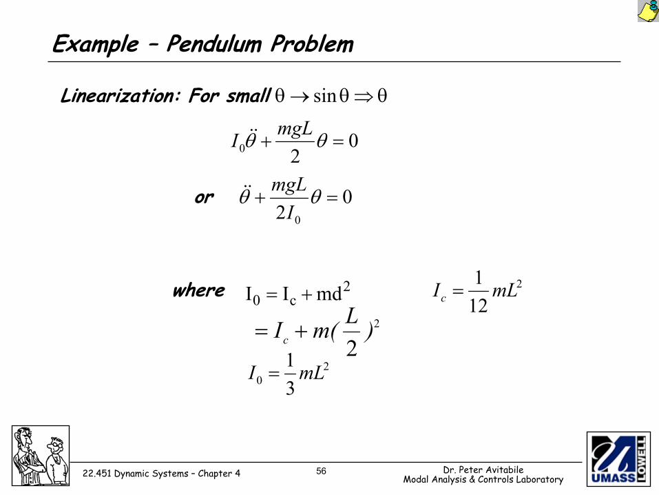
Linearization: For small
where 2c0 mdII +=
or
θ⇒θ→θ sin
020 =+ θθ mgLI &&
02 0
=+ θθImgL&&
2
2)Lm(Ic +=
20 31mLI =
2
121 mLIc =
Example – Pendulum Problem
57 Dr. Peter AvitabileModal Analysis & Controls Laboratory22.451 Dynamic Systems – Chapter 4
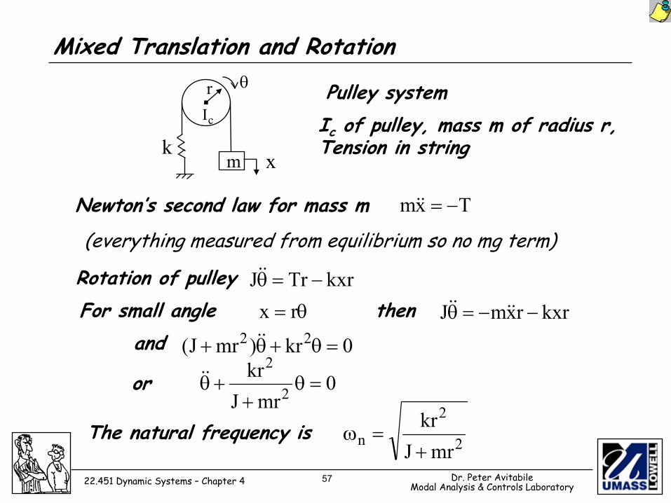
Mixed Translation and Rotation
Pulley system
Rotation of pulley
Newton’s second law for mass m
and
Txm −=&&
Ic of pulley, mass m of radius r, Tension in string
m x
r θ
kcI
(everything measured from equilibrium so no mg term)
For small angle
or
The natural frequency is
kxrTrJ −=θ&&
θ= rx kxrrxmJ −−=θ &&&&then
0kr)mrJ( 22 =θ+θ+ &&
0mrJkr
2
2=θ
++θ&&
2
2
n mrJkr+
=ω
58 Dr. Peter AvitabileModal Analysis & Controls Laboratory22.451 Dynamic Systems – Chapter 4
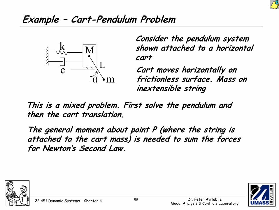
Example – Cart-Pendulum Problem
Consider the pendulum system shown attached to a horizontal cart
This is a mixed problem. First solve the pendulum and then the cart translation.
Cart moves horizontally on frictionless surface. Mass on inextensible string
The general moment about point P (where the string is attached to the cart mass) is needed to sum the forces for Newton’s Second Law.
M
c L
θ
k
m
59 Dr. Peter AvitabileModal Analysis & Controls Laboratory22.451 Dynamic Systems – Chapter 4
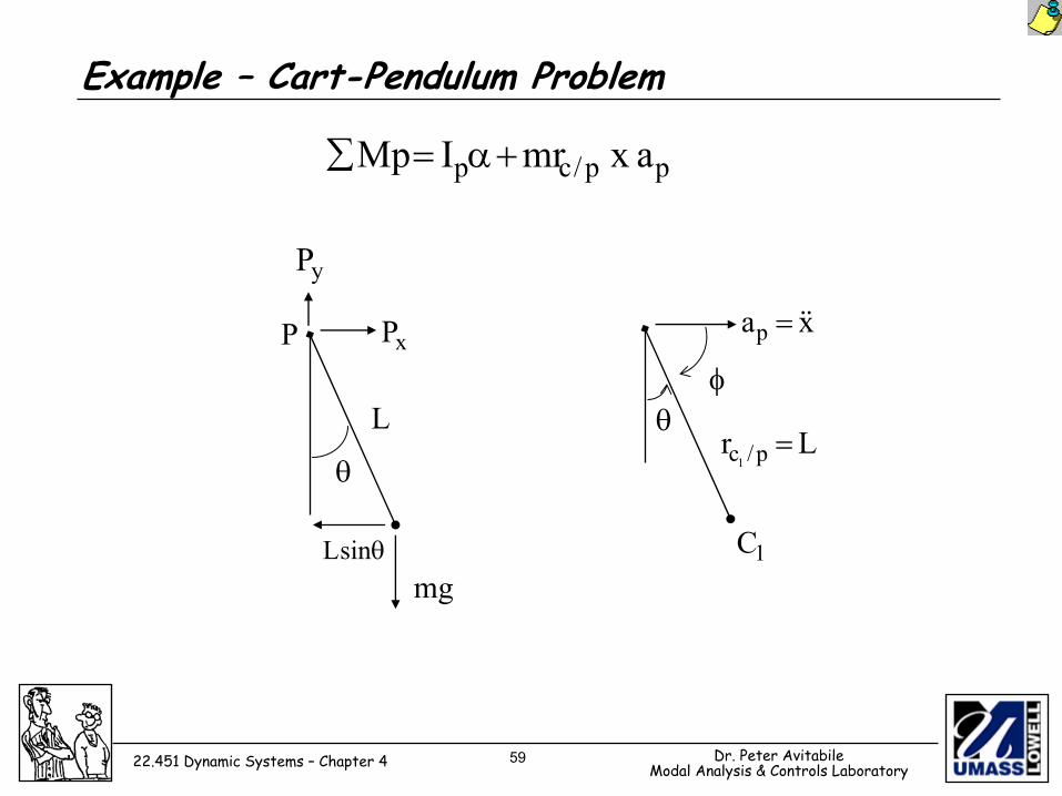
pp/cp axmrIMp +α=∑
yP
xPP
L
θ
mgθsinL
xap &&=
Lr p/c1 =
1C
θφ
Example – Cart-Pendulum Problem
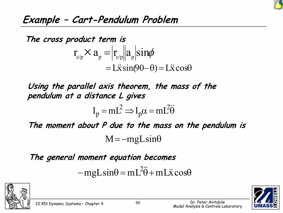
60 Dr. Peter AvitabileModal Analysis & Controls Laboratory22.451 Dynamic Systems – Chapter 4
The cross product term is
Using the parallel axis theorem, the mass of the pendulum at a distance L gives
The moment about P due to the mass on the pendulum isθ=α⇒= &&2
p2
p mLImLI
θ−= sinLmgM
φsinarar pc/ppc/p =×θ=θ−= cosxL)90sin(xL &&&&
The general moment equation becomes
θ+θ=θ− cosxLmLmsinLmg 2 &&&&
Example – Cart-Pendulum Problem
61 Dr. Peter AvitabileModal Analysis & Controls Laboratory22.451 Dynamic Systems – Chapter 4
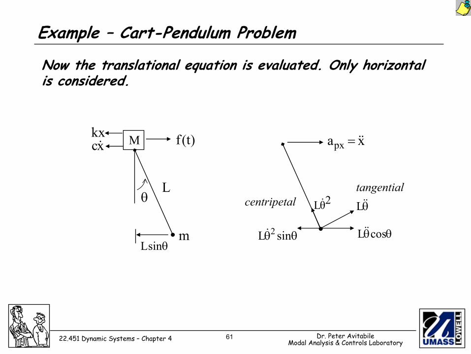
Now the translational equation is evaluated. Only horizontal is considered.
M )t(fkx
Lθ
mθsinL
xc& xapx &&=
2θL& θ&&L
θθ sinL 2& θθcosL&&
centripetaltangential
Example – Cart-Pendulum Problem
62 Dr. Peter AvitabileModal Analysis & Controls Laboratory22.451 Dynamic Systems – Chapter 4
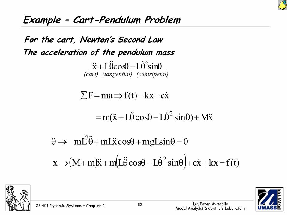
For the cart, Newton’s Second Law
xckx)t(fmaF &−−⇒=∑
The acceleration of the pendulum masssinθθLcosθθLx 2&&&&& −+
(cart) (tangential) (centripetal)
xM)sinLcosLx(m 2 &&&&&&& +θθ−θθ+=
0sinmgLcosxmLmL2 =θ+θ+θ→θ &&&&
( ) ( ) )t(fkxxcsinLcosLmxmMx 2 =++θθ−θθ++→ &&&&&&
Example – Cart-Pendulum Problem
63 Dr. Peter AvitabileModal Analysis & Controls Laboratory22.451 Dynamic Systems – Chapter 4
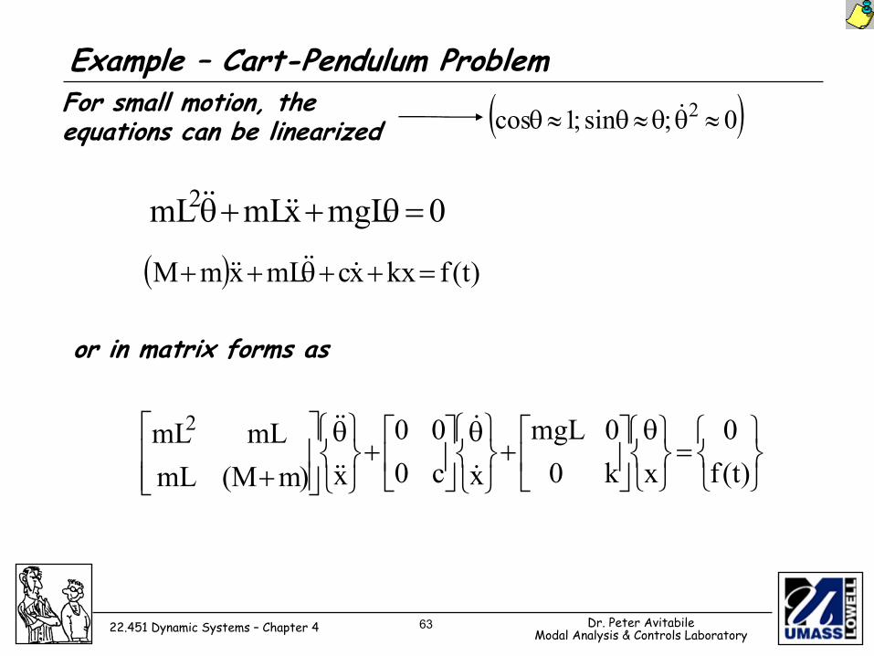
For small motion, the equations can be linearized
0mgLxmLmL2 =θ++θ &&&&
or in matrix forms as
( )0;sin;1cos 2 ≈θθ≈θ≈θ &
( ) )t(fkxxcmLxmM =++θ++ &&&&&
=
θ
+
θ
+
θ
+ )t(f0
xk00mgL
xc000
x)mM(mLmLmL2
&
&
&&
&&
Example – Cart-Pendulum Problem
64 Dr. Peter AvitabileModal Analysis & Controls Laboratory22.451 Dynamic Systems – Chapter 4
Chapter 4 - Review Slide
k2
x
f
k1
21eq kkk +=
k2
x1
f
k1
x2
21
21eq kk
kkk+
=
πζ≅ 2xxln2
1x1 x2 xn
t1 t2 tn
T