3.4 The Solow Model: Population Growth and Technological ... · PDF fileProf. Dr. Frank...
51
AVWL II Prof. Dr. Frank Heinemann Seite 1 3.4 The Solow Model: Population Growth and Technological Progress GDP Y t = F(K t , A t N t ) Labor efficiency A t Saving s Y t Consumption C t = (1 – s) Y t Depreciation δ K t Change of capital stocks over time: K t+1 –K t = s Y t – δ K t Population growth N t+1 = (1+n) N t Population growth rate n Technological progress A t+1 = (1+g) A t Rate of technological progress g
Transcript of 3.4 The Solow Model: Population Growth and Technological ... · PDF fileProf. Dr. Frank...
AVWL II Prof. Dr. Frank Heinemann Seite 1
3.4 The Solow Model: Population Growth and Technological Progress
GDP
Yt
= F(Kt
, At
Nt
)Labor efficiency At
Saving s Yt
Consumption
Ct
= (1 –
s) Yt
Depreciation
δ
Kt
Change of capital stocks over time:Kt+1
– Kt = s Yt
–
δ
Kt
Population growth
Nt+1
= (1+n) NtPopulation growth rate
n
Technological progress
At+1
= (1+g) AtRate of technological progress
g
AVWL II Prof. Dr. Frank Heinemann Seite 2
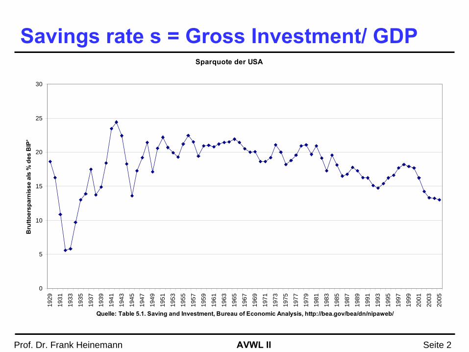
Savings rate s = Gross Investment/ GDPSparquote der USA
0
5
10
15
20
25
30
1929
1931
1933
1935
1937
1939
1941
1943
1945
1947
1949
1951
1953
1955
1957
1959
1961
1963
1965
1967
1969
1971
1973
1975
1977
1979
1981
1983
1985
1987
1989
1991
1993
1995
1997
1999
2001
2003
2005
Quelle: Table 5.1. Saving and Investment, Bureau of Economic Analysis, http://bea.gov/bea/dn/nipaweb/
Bru
ttoer
spar
niss
e al
s %
des
BIP
'
AVWL II Prof. Dr. Frank Heinemann Seite 3
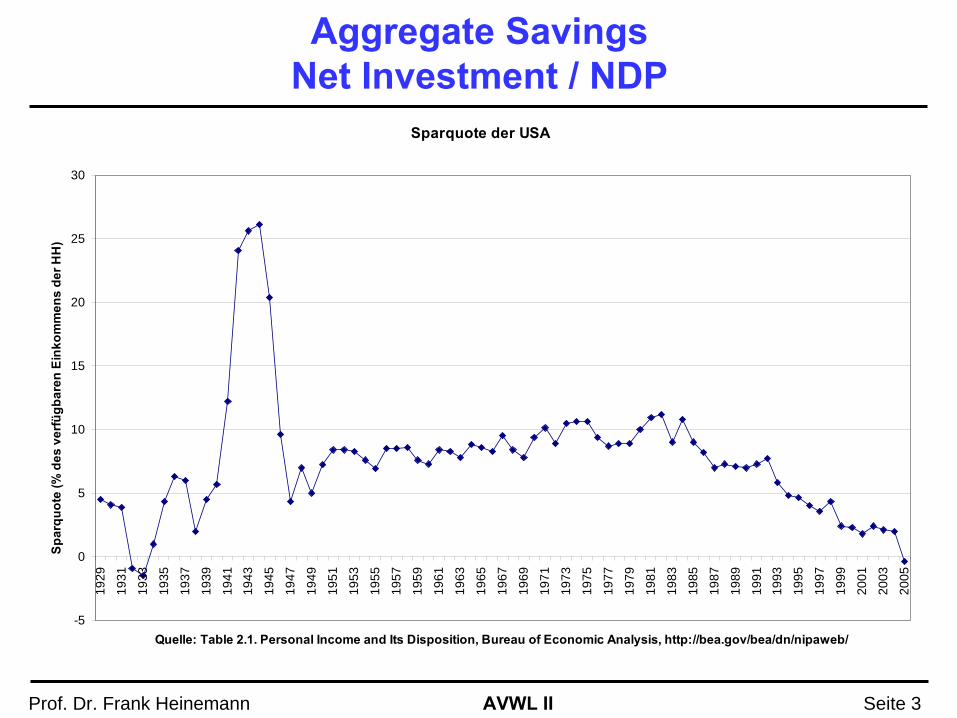
Aggregate Savings Net Investment / NDP
Sparquote der USA
-5
0
5
10
15
20
25
30
1929
1931
1933
1935
1937
1939
1941
1943
1945
1947
1949
1951
1953
1955
1957
1959
1961
1963
1965
1967
1969
1971
1973
1975
1977
1979
1981
1983
1985
1987
1989
1991
1993
1995
1997
1999
2001
2003
2005
Quelle: Table 2.1. Personal Income and Its Disposition, Bureau of Economic Analysis, http://bea.gov/bea/dn/nipaweb/
Spar
quot
e (%
des
ver
fügb
aren
Ein
kom
men
s de
r HH
)
AVWL II Prof. Dr. Frank Heinemann Seite 4
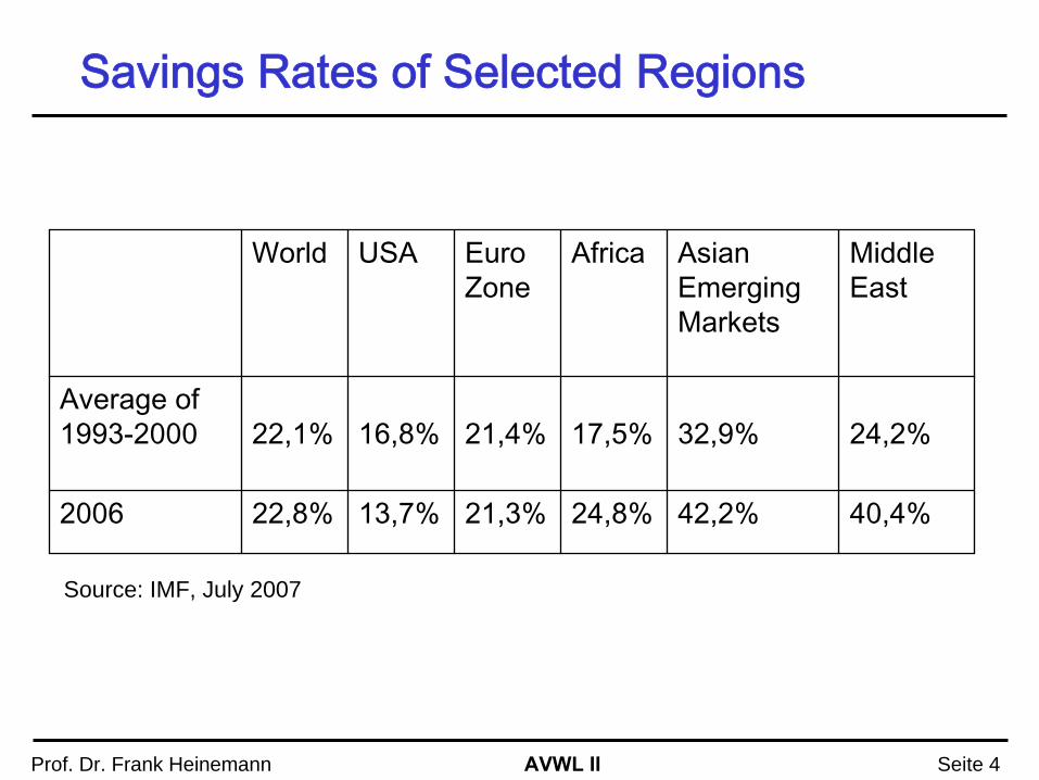
Savings Rates of Selected Regions
World USA Euro Zone
Africa Asian Emerging Markets
Middle East
Average of 1993-2000 22,1% 16,8% 21,4% 17,5% 32,9% 24,2%
2006 22,8% 13,7% 21,3% 24,8% 42,2% 40,4%
Source: IMF, July 2007
AVWL II Prof. Dr. Frank Heinemann Seite 5
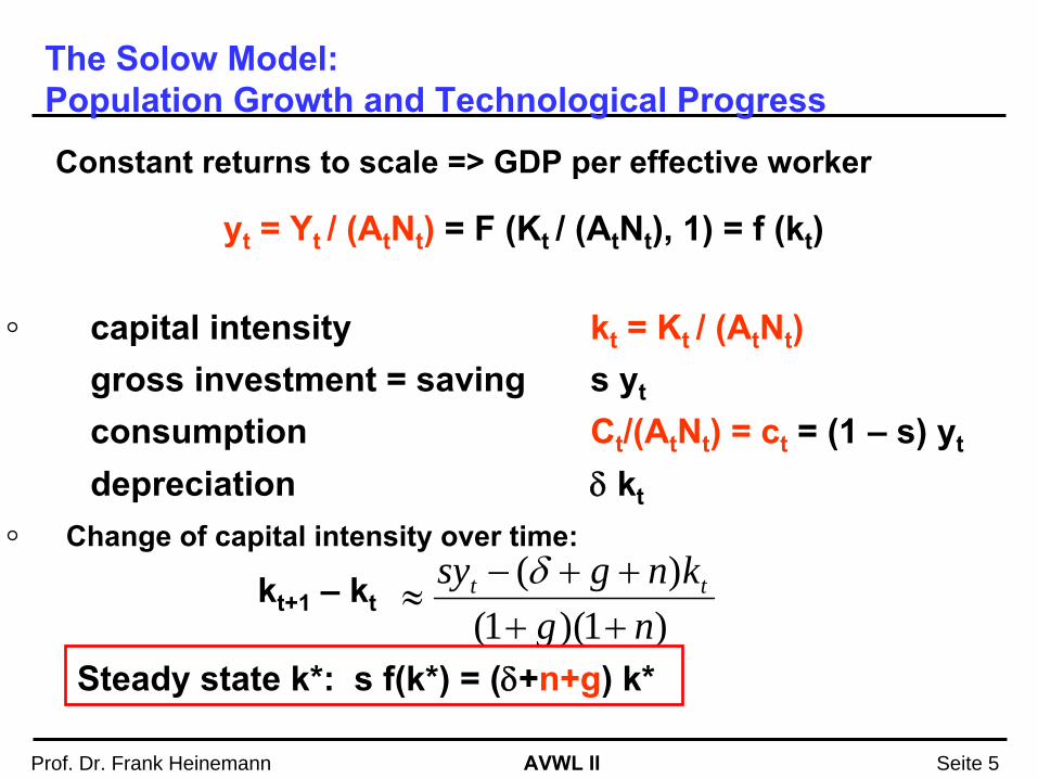
The Solow Model: Population Growth and Technological Progress
Constant returns to scale => GDP per effective worker
Change of capital intensity over time:
kt+1
– kt
capital intensity
kt
= Kt / (At
Nt
)gross investment = saving s yt
consumption
Ct
/(At
Nt
) = ct
= (1 –
s) yt
depreciation δ
kt
yt
= Yt
/ (At
Nt
)
= F (Kt / (At
Nt
), 1) = f (kt
)
)1()1()(
ngkngsy tt
++++−
≈δ
Steady state k*: s f(k*) = (δ+n+g) k*
AVWL II Prof. Dr. Frank Heinemann Seite 6
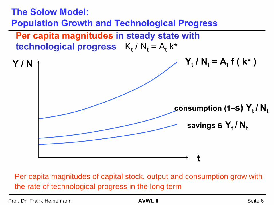
The Solow Model: Population Growth and Technological Progress
Per capita magnitudes in steady state with technological progress
t
Per capita magnitudes of capital stock, output and consumption grow with the rate of technological progress in the long term
Kt / Nt = At k*
Y / N Yt
/ Nt
= At
f ( k* )
savings
s Yt
/ Nt
consumption
(1–s) Yt
/ Nt
AVWL II Prof. Dr. Frank Heinemann Seite 7
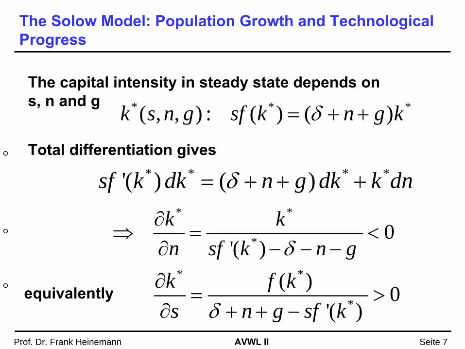
The Solow Model: Population Growth and Technological Progress
The capital intensity in steady state depends on s, n and g * * *( , , ) : ( ) ( )k s n g sf k n g kδ= + +
Total differentiation gives* * * *'( ) ( )sf k dk n g dk k dnδ= + + +
* *
* 0'( )
k kn sf k n gδ
∂⇒ = <
∂ − − −* *
*
( ) 0'( )
k f ks n g sf kδ
∂= >
∂ + + −equivalently
AVWL II Prof. Dr. Frank Heinemann Seite 8
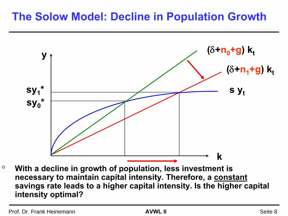
The Solow Model: Decline in Population Growth
k
y(δ+n1
+g) kt
With a decline in growth of population, less investment is necessary to maintain capital intensity. Therefore, a constant
savings rate leads to a higher capital intensity. Is the higher capital intensity optimal?
s ytsy0
*sy1
*
(δ+n0
+g) kt
AVWL II Prof. Dr. Frank Heinemann Seite 9
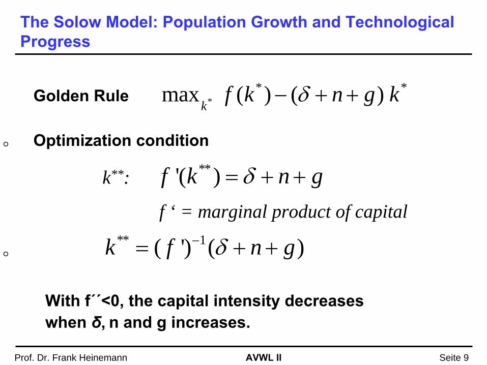
The Solow Model: Population Growth and Technological Progress
Golden Rule
**'( )f k n gδ= + +
Optimization condition
f ‘ = marginal product of capital
** *max ( ) ( )
kf k n g kδ− + +
k**:
** 1( ') ( )k f n gδ−= + +
With f´´<0, the capital intensity decreases when δ,
n and g increases.
AVWL II Prof. Dr. Frank Heinemann Seite 10
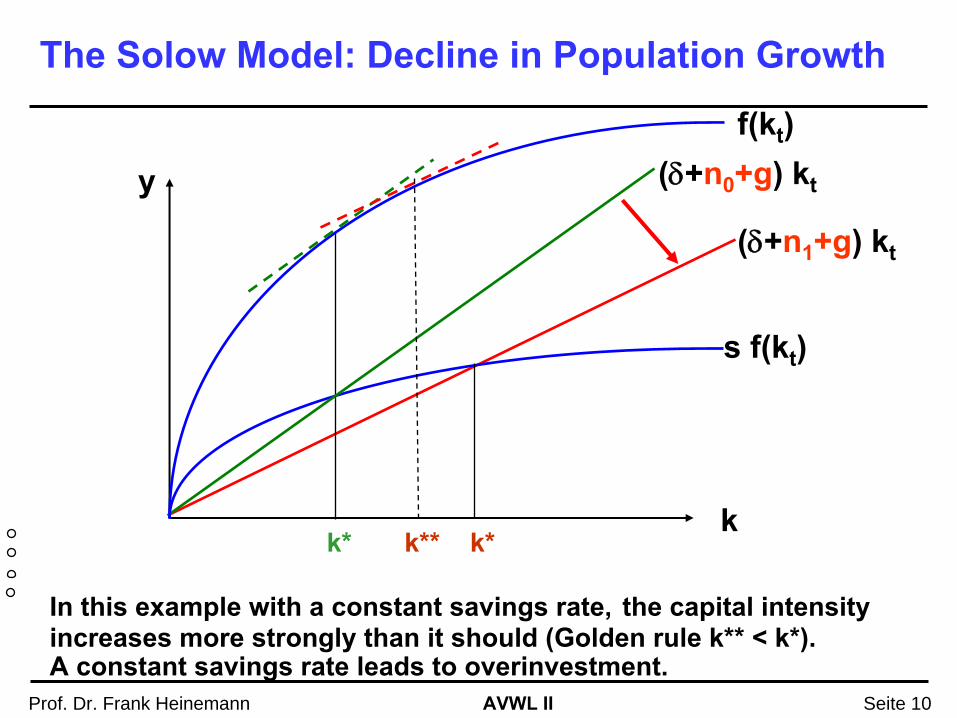
The Solow Model: Decline in Population Growth
k
y
(δ+n1
+g) kt
In this example with a constant savings rate,
the capital intensity increases more strongly than it should (Golden rule k** < k*). A constant savings rate leads to overinvestment.
s f(kt
)
(δ+n0
+g) kt
f(kt
)
k*k**k*
AVWL II Prof. Dr. Frank Heinemann Seite 11
The Solow Model: Decline in Population Growth
On the one hand, capital intensity should increase, when n decreases.
On the other hand, the decline in population growth automatically leads to an increase in capital intensity with a constant saving rate.
How does the savings rate react to a decline in population growth?
AVWL II Prof. Dr. Frank Heinemann Seite 12
The Solow Model: Decline in Population Growth
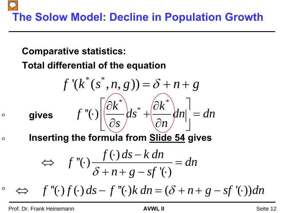
Total differential of the equation
* **''( ) k kf ds dn dn
s n⎡ ⎤∂ ∂
⋅ + =⎢ ⎥∂ ∂⎣ ⎦
Comparative statistics:
* *'( ( , , ))f k s n g n gδ= + +
( )''( )'( )
f ds k dnf dnn g sfδ⋅ −
⇔ ⋅ =+ + − ⋅
gives
''( ) ( ) ''( ) ( '( ))f f ds f k dn n g sf dnδ⇔ ⋅ ⋅ − ⋅ = + + − ⋅
Inserting
the
formula
from
Slide
54
gives
Vorführender
Präsentationsnotizen
Woran sieht man das? Gehe zurück zum Bild des steady state und erkläre es daran.
AVWL II Prof. Dr. Frank Heinemann Seite 13
The Solow Model: Decline in Population Growth
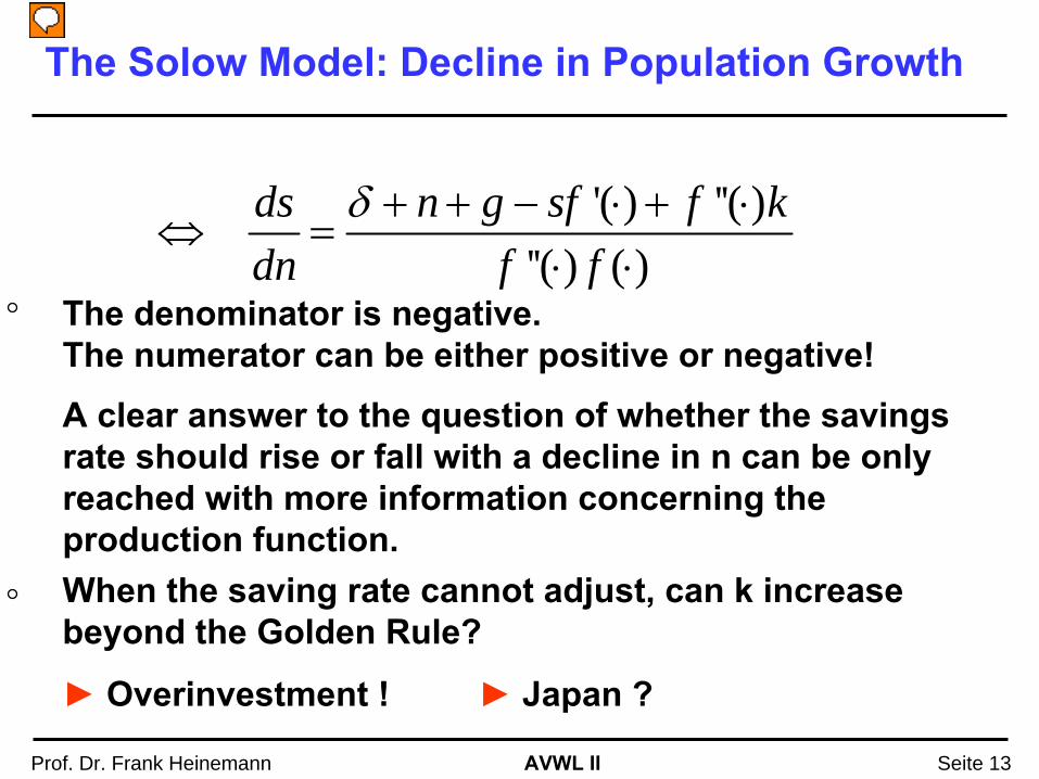
'( ) ''( )''( ) ( )
ds n g sf f kdn f f
δ + + − ⋅ + ⋅⇔ =
⋅ ⋅The denominator is negative. The numerator can be either positive or negative!
A clear answer to the question of whether the savings rate should rise or fall with a decline in n can be only reached with more information concerning the production function. When the saving rate cannot adjust, can k increase beyond the Golden Rule?
► Overinvestment ! ► Japan ?
Vorführender
Präsentationsnotizen
Woran sieht man das? Gehe zurück zum Bild des steady state und erkläre es daran.
AVWL II Prof. Dr. Frank Heinemann Seite 14
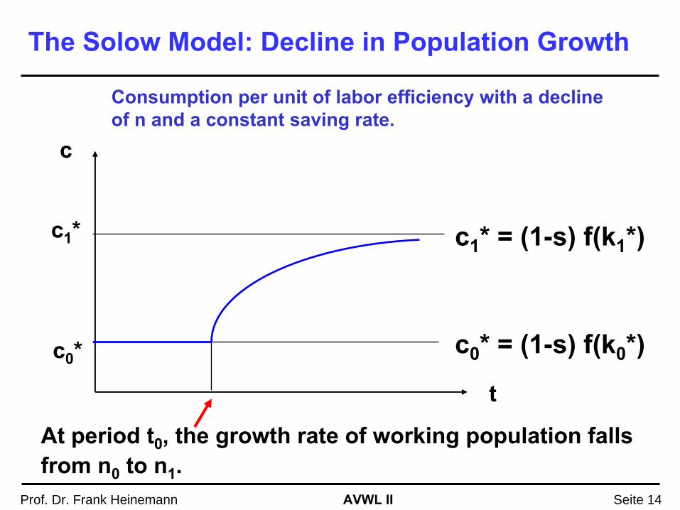
The Solow Model: Decline in Population Growth
Consumption per unit of labor efficiency with a decline of n and a constant saving rate.
t
c
At period t0
, the growth rate of working population falls from n0
to n1
.
c0
*
c1
* c1
* = (1-s) f(k1
*)
c0
* = (1-s) f(k0
*)
AVWL II Prof. Dr. Frank Heinemann Seite 15
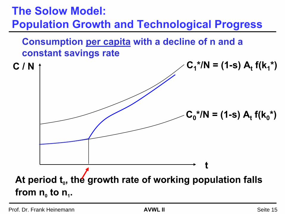
The Solow Model: Population Growth and Technological Progress
t
C / N
C0
*/N = (1-s) At
f(k0
*)
C1
*/N = (1-s) At
f(k1
*)
Consumption per capita
with a decline of n and a constant savings rate
At period t0
, the growth rate of working population falls from n0
to n1
.
AVWL II Prof. Dr. Frank Heinemann Seite 16
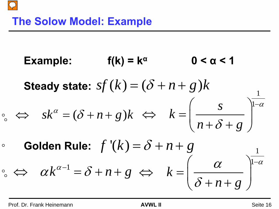
The Solow Model: Example
Example: f(k) = kα
0 < α
< 1
Steady state: ( ) ( )sf k n g kδ= + +
( )sk n g kα δ⇔ = + +
1k n gαα δ−⇔ = + +
'( )f k n gδ= + +
11sk
n g
α
δ
−⎛ ⎞⇔ = ⎜ ⎟+ +⎝ ⎠
Golden Rule: 11
kn g
ααδ
−⎛ ⎞⇔ = ⎜ ⎟+ +⎝ ⎠
Vorführender
Präsentationsnotizen
Woran sieht man das? Gehe zurück zum Bild des steady state und erkläre es daran.
AVWL II Prof. Dr. Frank Heinemann Seite 17
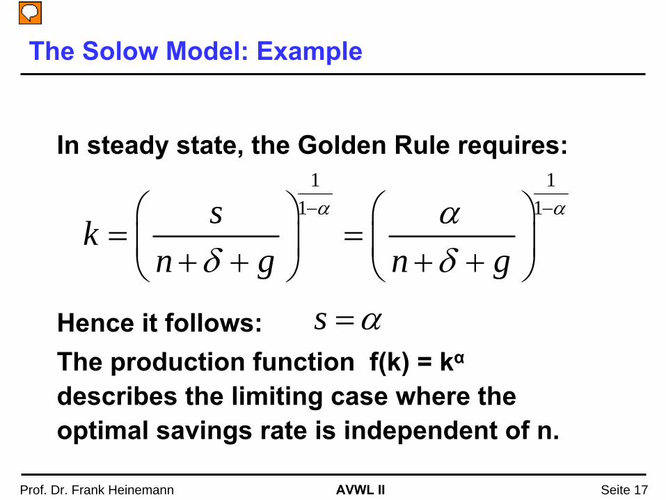
The Solow Model: Example
In steady state, the Golden Rule requires:
s α=
1 11 1sk
n g n g
α ααδ δ
− −⎛ ⎞ ⎛ ⎞= =⎜ ⎟ ⎜ ⎟+ + + +⎝ ⎠ ⎝ ⎠
Hence it follows:The production function f(k) = kα
describes the limiting case where the optimal savings rate is independent of n.
Vorführender
Präsentationsnotizen
Woran sieht man das? Gehe zurück zum Bild des steady state und erkläre es daran.
AVWL II Prof. Dr. Frank Heinemann Seite 18
The Solow ModelThe Solow model describes the optimal saving in steady state.
The adjustment process takes time though. The Solow model does not describe the optimal adjustment track.
The ‘optimal saving rate’
maximizes the per capita consumption in steady state. The steady state will never be completely reached.
Time preference: future consumption should be discounted. Consumption during the adjustment phase must be considered.
These critiques are considered by Ramsey model. Recession studies: business cycles, growth and employment
Vorführender
Präsentationsnotizen
Woran sieht man das? Gehe zurück zum Bild des steady state und erkläre es daran.
AVWL II Prof. Dr. Frank Heinemann Seite 19
Technological Progress
3.5. The role of technological progress in the process of growth
3.6. Determinants of the technological progress 3.6.a) Optimal patent protection
3.7. Distribution effects of technological progress
Literature:
Blanchard, Chapter 12-13.Burda
& Wyplosz, Macroeconomics, 3rd. ed. Oxford
Univ. Press 2001, Chapter 18
Abel & Bernanke, Macroeconomics, 5th ed., Chapter 6
AVWL II Prof. Dr. Frank Heinemann Seite 20
Technological Progress
Dimensions of technological progress:
Higher productivity of the factors capital and labor
Better products
New products
A larger variety of products
AVWL II Prof. Dr. Frank Heinemann Seite 21
3.5 Growth and Technological Progress
Production function Y = F(K,AN) = Ka
(AN)1-a
GDP growth rate dYt
/Yt
Rate of technological progress g = dAt
/At
Growth rate of working population
n = dNt
/Nt
Per effective worker y = f(k) = ka.
Steady State (Solow): sf(k*) = δ
+ n + g .
k converges to k* and y to y*.
AVWL II Prof. Dr. Frank Heinemann Seite 22
Growth and Technological Progress
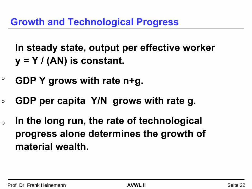
In steady state, output per effective worker y = Y / (AN) is constant.
GDP Y grows with rate n+g.
GDP per capita Y/N grows with rate g.
In the long run, the rate of technological progress alone determines the growth of material wealth.

AVWL II Prof. Dr. Frank Heinemann Seite 23
Growth and Technological Progress
Growth of Output per Capita
Rate of Technological Progress
1950-73
1973-87
Change
1950-73
1973-87
Change (1)
(2)
(3)
(4)
(5)
(6)
France
4.0
1.8
-2.2
4.9
2.3
-2.6
Germany
4.9
2.1
-2.8
5.6
1.9
-3.7
Japan
8.0
3.1
-4.9
6.4
1.7
-4.7
United Kingdom
2.5
1.8
-0.7
2.3
1.7
-0.6
United States
2.2
1.6
-0.6
2.6
0.6
-2.0
Average
4.3
2.1
-2.2
4.4
1.6
-2.8
AVWL II Prof. Dr. Frank Heinemann Seite 24
Growth and Technological Progress
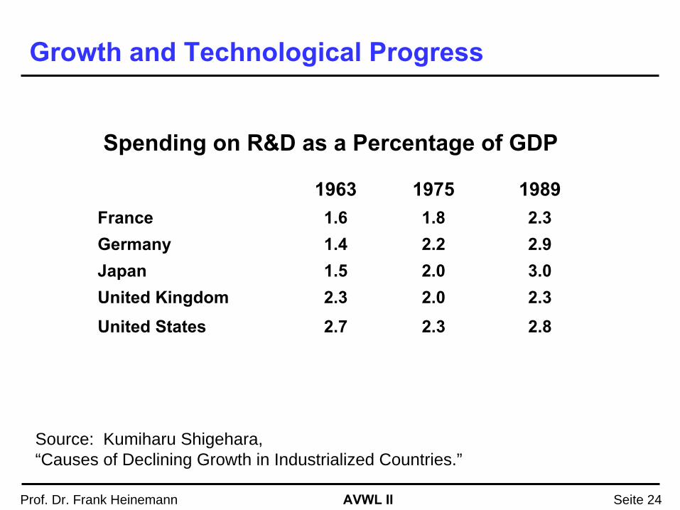
1963 1975
1989
France
1.6
1.8
2.3Germany
1.4
2.2
2.9
Japan
1.5
2.0
3.0United Kingdom
2.3
2.0
2.3
United States
2.7
2.3
2.8
Source: Kumiharu Shigehara, “Causes of Declining Growth in Industrialized Countries.”
Spending on R&D as a Percentage of GDP
AVWL II Prof. Dr. Frank Heinemann Seite 25
Growth and Technological Progress
Evidence:Rate of technological progress has declined.However, the fraction of expenditure on research
and development has not declined. Has the research process become inefficient?
AVWL II Prof. Dr. Frank Heinemann Seite 26
Growth and Technological Progress
Errors in measurement:Product quality and variety need findings from research and development that do not necessarily increase GDP with competitive prices.
Example: electronic equipmentsImprovement in capacity with constant price.
Capacity characteristics do not agree with price comparison. Consequences: Overestimation of inflation, underestimation
of technological progress.
AVWL II Prof. Dr. Frank Heinemann Seite 27
Growth and
Technological Progress
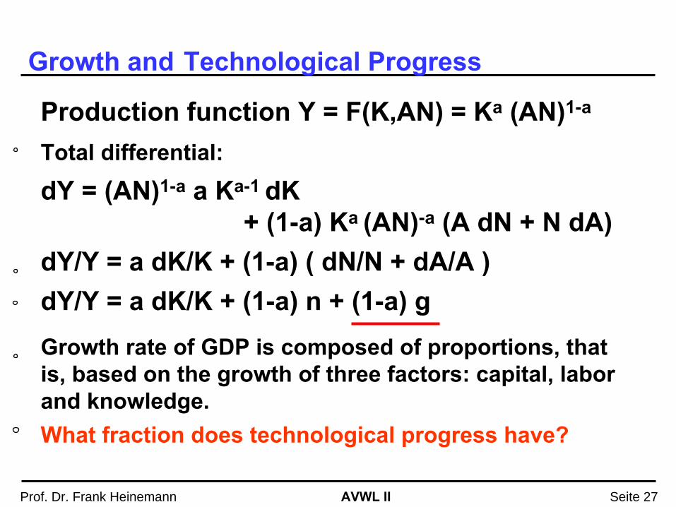
Production function Y = F(K,AN) = Ka
(AN)1-a
Total differential:
dY
= (AN)1-a
a Ka-1 dK + (1-a) Ka (AN)-a
(A dN
+ N dA)
dY/Y = a dK/K + (1-a) ( dN/N + dA/A )dY/Y = a dK/K + (1-a) n + (1-a) gGrowth rate of GDP is composed of proportions, that is, based on the growth of three factors: capital, labor and knowledge.What fraction does technological progress have?
AVWL II Prof. Dr. Frank Heinemann Seite 28
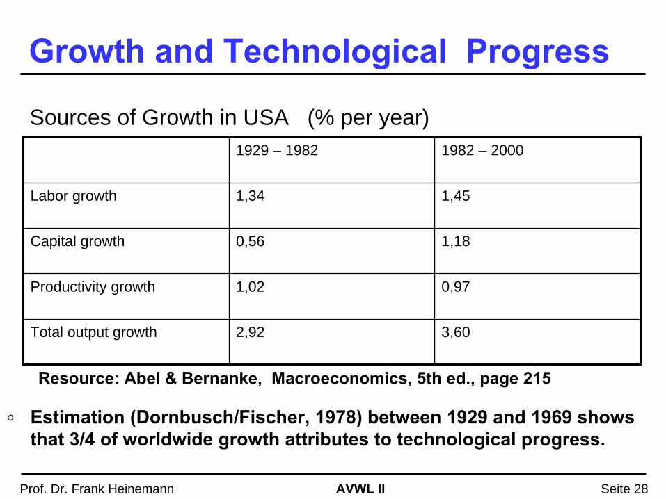
Growth and Technological Progress
Sources of Growth in USA (% per year)1929 – 1982 1982 – 2000
Labor growth 1,34 1,45
Capital growth 0,56 1,18
Productivity growth 1,02 0,97
Total output growth 2,92 3,60
Resource: Abel & Bernanke, Macroeconomics, 5th ed., page 215
Estimation (Dornbusch/Fischer, 1978) between 1929 and 1969 shows that 3/4 of worldwide growth attributes to technological progress.
AVWL II Prof. Dr. Frank Heinemann Seite 29
Growth and Technological Progress
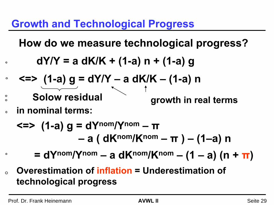
How do we measure technological progress?dY/Y = a dK/K + (1-a) n + (1-a) g
<=> (1-a) g = dY/Y –
a dK/K –
(1-a) nSolow residual
in nominal terms:<=> (1-a) g = dYnom/Ynom
–
π
– a ( dKnom/Knom
–
π
) –
(1–a) n= dYnom/Ynom
– a dKnom/Knom
– (1 – a) (n + π)
Overestimation of inflation
= Underestimation of technological progress
growth in real terms
AVWL II Prof. Dr. Frank Heinemann Seite 30
3.6 Determinants of Technological Progress
Technological progress is not exogenous.
Where does technological progress arise from?
How is the cost-benefit analysis of the decision maker?
Is the level of research and development efficient?
AVWL II Prof. Dr. Frank Heinemann Seite 31
Determinants of Technological Progress
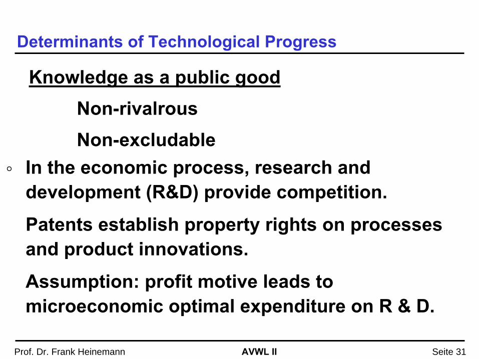
Knowledge as a public goodNon-rivalrousNon-excludable
In the economic process, research and development (R&D) provide competition.
Patents establish property rights on processes and product innovations.
Assumption: profit motive leads to microeconomic optimal expenditure on R & D.
AVWL II Prof. Dr. Frank Heinemann Seite 32
Determinants of Technological Progress
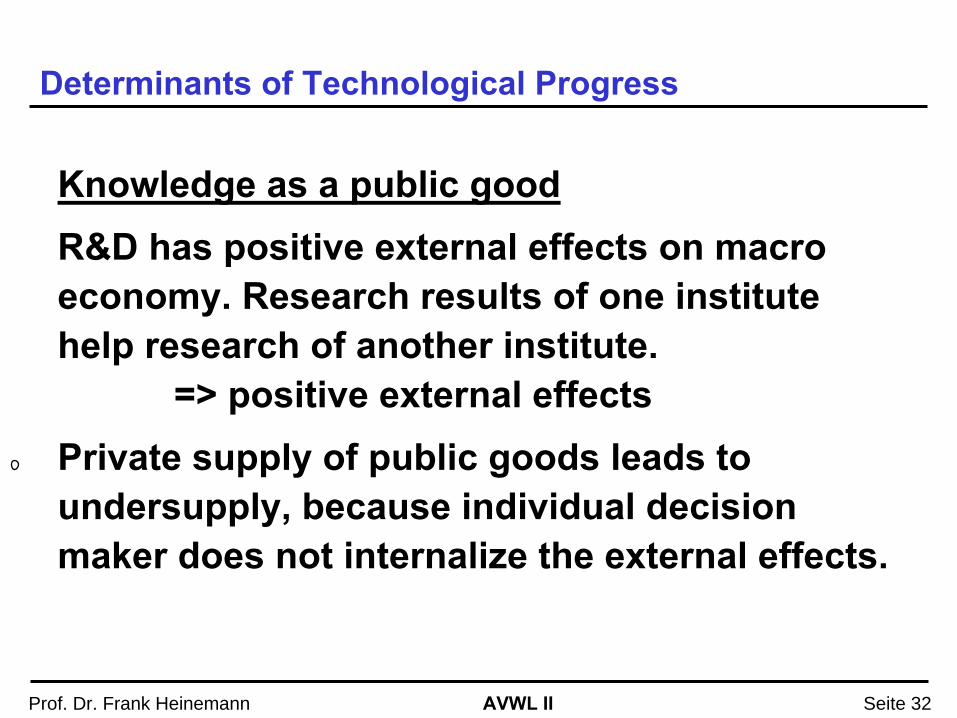
Knowledge as a public goodR&D has positive external effects on macro economy. Research results of one institute help research of another institute.
=> positive external effectsPrivate supply of public goods leads to undersupply, because individual decision maker does not internalize the external effects.
AVWL II Prof. Dr. Frank Heinemann Seite 33
Determinants of Technological Progress
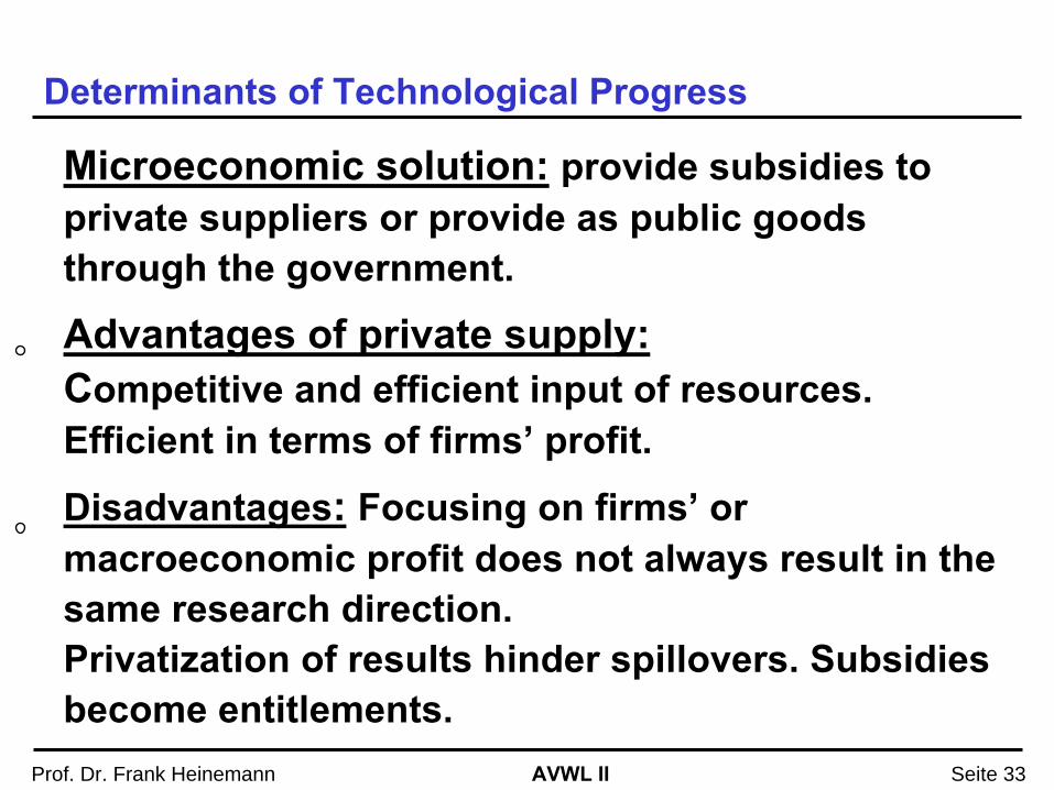
Microeconomic solution:
provide subsidies to private suppliers or provide as public goods through the government.
Advantages of private supply: Competitive and efficient input of resources.
Efficient in terms of firms’
profit.
Disadvantages:
Focusing on firms’
or macroeconomic profit does not always result in the same research direction. Privatization of results hinder spillovers. Subsidies become entitlements.
AVWL II Prof. Dr. Frank Heinemann Seite 34
Determinants of Technological Progress
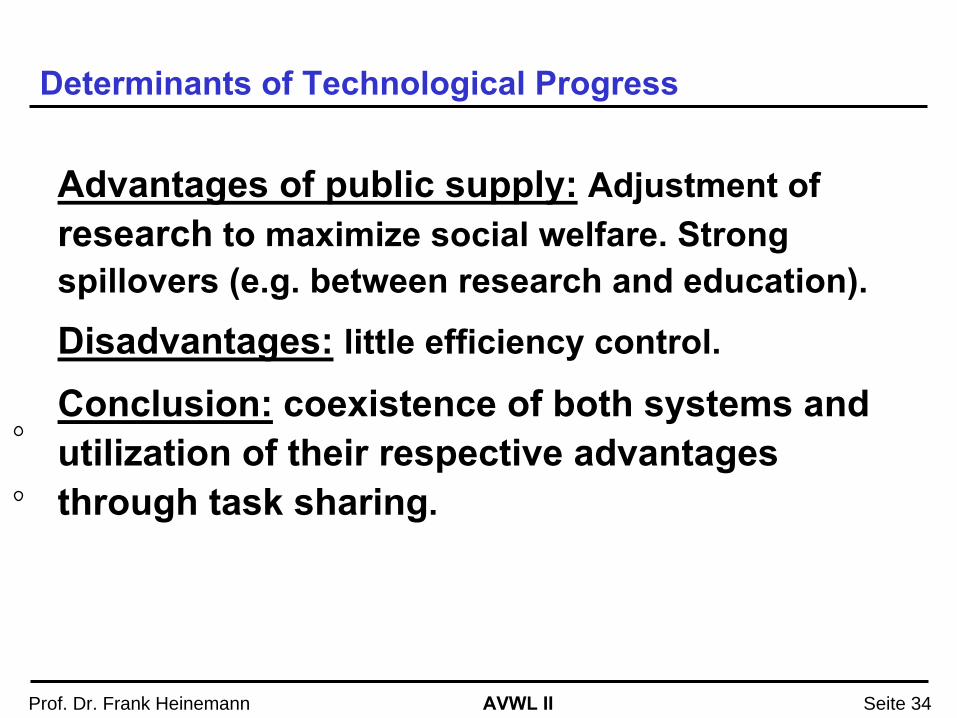
Advantages of public supply:
Adjustment of research
to maximize social welfare. Strong
spillovers (e.g. between research and education).
Disadvantages:
little efficiency control.
Conclusion:
coexistence of both systems and utilization of their respective advantages through task sharing.
AVWL II Prof. Dr. Frank Heinemann Seite 35
3.6.a) Optimal Patent Protection
Product innovations are directly evaluated on the market. Clear measure of value. Patents hinder product competition and lead to higher price, lower consumer surplus, and monopolistic profit of firms. => inefficiencyAn the same time, monopolistic profit stimulates firms to invest in R&D.Optimal patent protection must balance the trade-
off between positive effects on stimulation of R&D, and welfare gains from spillover effects.
AVWL II Prof. Dr. Frank Heinemann Seite 36
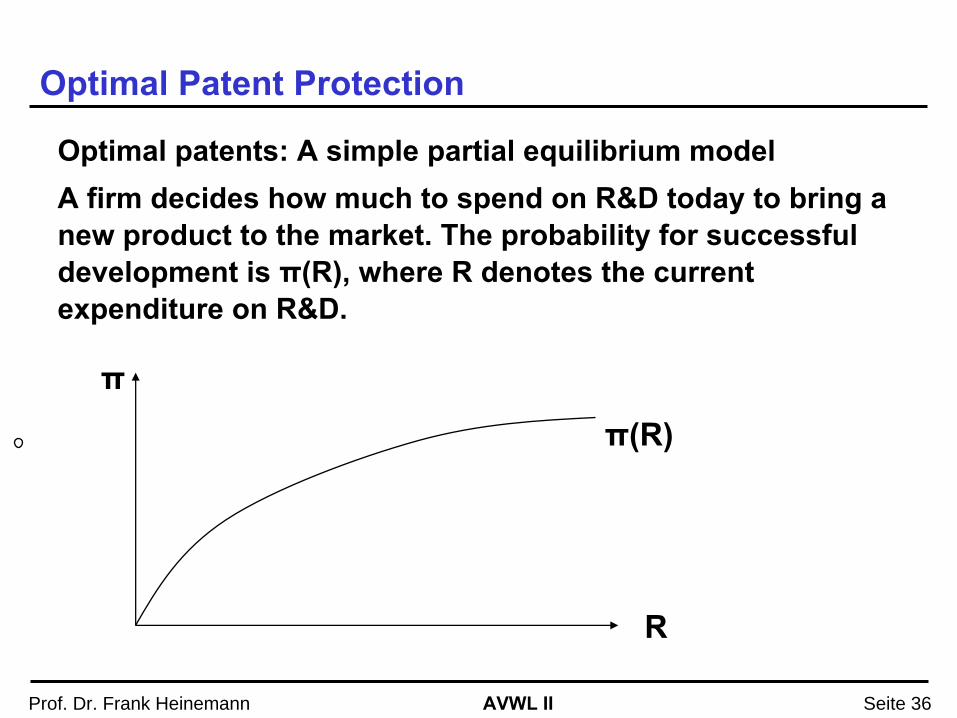
Optimal Patent Protection
Optimal patents: A simple partial equilibrium modelA firm decides how much to spend on R&D today to bring a new product to the market. The probability for successful development is π(R), where R denotes the current expenditure on R&D.
π
R
π(R)
AVWL II Prof. Dr. Frank Heinemann Seite 37
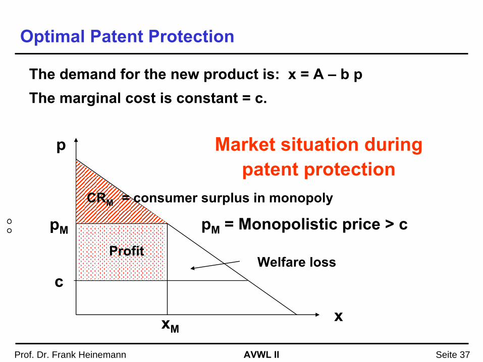
Optimal Patent Protection
The demand for the new product is: x = A –
b pThe marginal cost is constant = c.
p
x
Market situation during patent protection
xM
pM
cWelfare loss
pM
= Monopolistic price > cCRM = consumer surplus in monopoly
Profit
AVWL II Prof. Dr. Frank Heinemann Seite 38
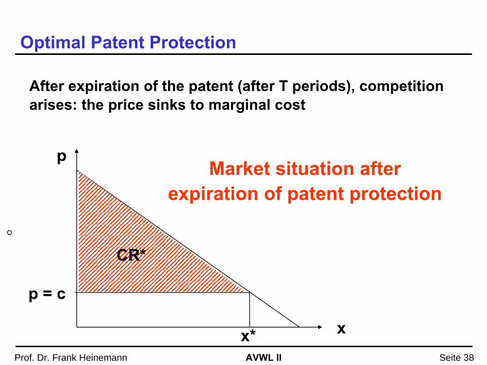
Optimal Patent Protection
p
x
Market situation after expiration of patent protection
x*
p = c
After expiration of the patent (after T periods), competition arises: the price sinks to marginal cost
CR*
AVWL II Prof. Dr. Frank Heinemann Seite 39
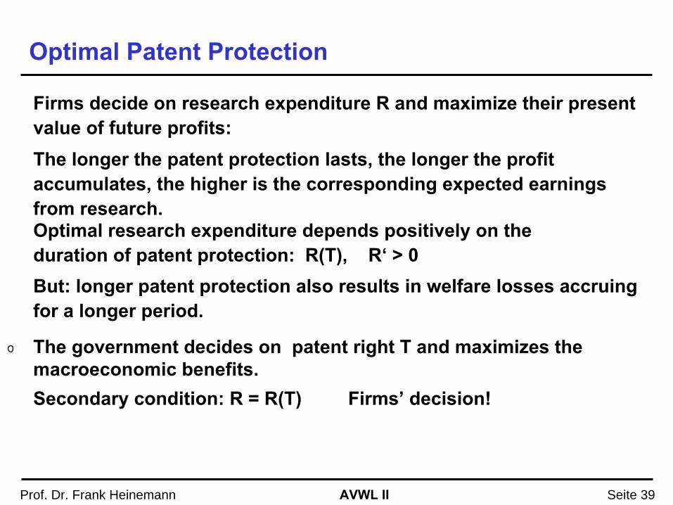
Optimal Patent Protection
Optimal research expenditure depends positively on the duration of patent protection: R(T), R‘
> 0
Firms decide on research expenditure R and maximize their present value of future profits:The longer the patent protection lasts, the longer the profit accumulates, the higher is the corresponding expected earnings from research.
But: longer patent protection also results in welfare losses accruing for a longer period.
The government decides on patent right T and maximizes the macroeconomic benefits.Secondary condition: R = R(T) Firms’
decision!
AVWL II Prof. Dr. Frank Heinemann Seite 40
Optimal Patent Protection
Notice: The optimal patent protection balances the trade-off between:
- Welfare loss that is caused by the monopolistic market: The longer the patent protection, the higher the loss.
- Welfare gain that arises as expected monopolistic profits stimulate innovations. Under short-term patent protection private R&D are not attractive. Innovations don’t occur!
AVWL II Prof. Dr. Frank Heinemann Seite 41
3.7 Technological Progress and Income Distribution
Two perceptions:Technological progress enhances output and thereby salaries.Process innovations set work force free and therefore degrade the wage rate in market equilibrium.Different types of technological progress
AVWL II Prof. Dr. Frank Heinemann Seite 42
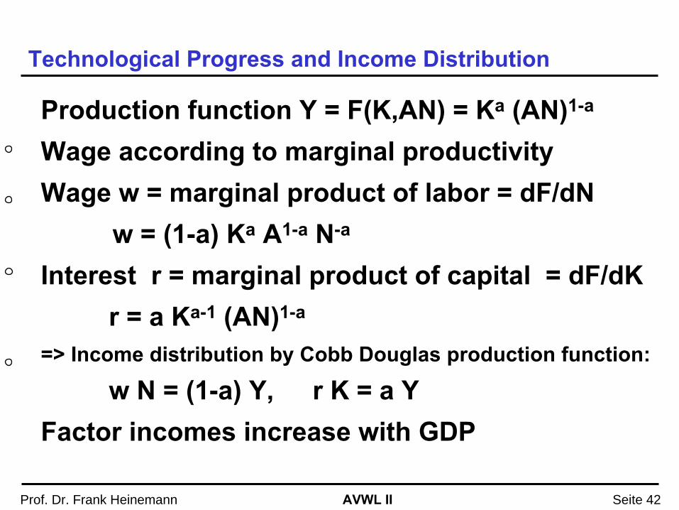
Technological Progress and Income Distribution
Production function Y = F(K,AN) = Ka
(AN)1-a
Wage according to marginal productivityWage w = marginal product of labor = dF/dN
w = (1-a) Ka
A1-a
N-a
Interest r = marginal product of capital = dF/dKr = a Ka-1
(AN)1-a
=> Income distribution by Cobb Douglas production function:
w N = (1-a) Y, r K = a YFactor incomes increase with GDP
AVWL II Prof. Dr. Frank Heinemann Seite 43
Technological Progress and Income Distribution
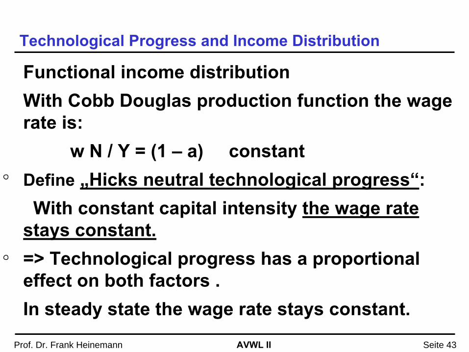
Functional income distributionWith Cobb Douglas production function the wage rate is:
w N / Y = (1 –
a) constant Define
„Hicks neutral technological progress“:
With constant capital intensity the wage rate stays constant. => Technological progress has a proportional effect on both factors .In steady state the wage rate stays constant.
AVWL II Prof. Dr. Frank Heinemann Seite 44
Technological Progress and Income Distribution
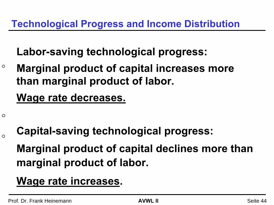
Labor-saving technological progress:Marginal product of capital increases more than marginal product of labor.Wage rate decreases.
Capital-saving technological progress:Marginal product of capital declines more than marginal product of labor.
Wage rate increases.
AVWL II Prof. Dr. Frank Heinemann Seite 45
Technological Progress and Income Distribution
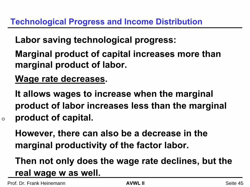
Labor saving technological progress:Marginal product of capital increases more than marginal product of labor.Wage rate decreases.It allows wages to increase when the marginal product of labor increases less than the marginal product of capital.
However, there can also be a decrease in the marginal productivity of the factor labor.
Then not only does the wage rate declines, but the real wage w as well.
AVWL II Prof. Dr. Frank Heinemann Seite 46
Technological Progress and Income Distribution
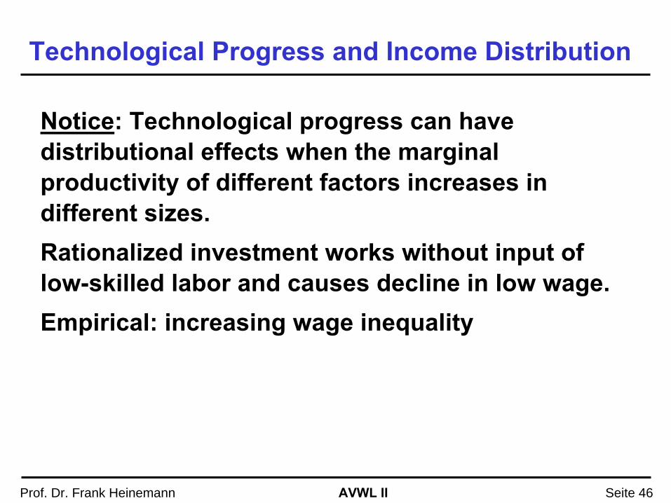
Notice: Technological progress can have distributional effects when the marginal productivity of different factors increases in different sizes.Rationalized investment works without input of low-skilled labor and causes decline in low wage. Empirical: increasing wage inequality
AVWL II Prof. Dr. Frank Heinemann Seite 47
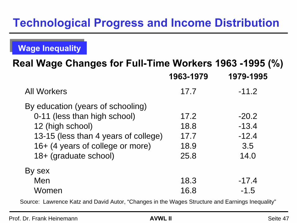
Technological Progress and Income Distribution
Wage InequalityWage Inequality
1963-1979
1979-1995
All Workers 17.7 -11.2
By education (years of schooling) 0-11 (less than high school) 17.2 -20.2 12 (high school) 18.8 -13.4 13-15 (less than 4 years of college) 17.7 -12.4 16+ (4 years of college or more) 18.9 3.5 18+ (graduate school) 25.8 14.0
By sex Men 18.3 -17.4 Women 16.8 -1.5
Source: Lawrence Katz and David Autor, “Changes in the Wages Structure and Earnings Inequality”
Real Wage Changes for Full-Time Workers 1963 -1995 (%)
AVWL II Prof. Dr. Frank Heinemann Seite 48
Technological Progress and Income Distribution
Reasons for increasing wage inequality:1. Globalization (Heckscher
Ohlin Samuelson theorem):
The wages of qualified labor become equal with free capital flow.In emerging markets, the fraction of low-skilled labor is larger than in developed countries.International competition squeezes the wages, particularly those of low-skilled workers.
Lecture in international economics, recession studies
AVWL II Prof. Dr. Frank Heinemann Seite 49
Technological Progress and Income Distribution
Reasons for increasing wage inequality:2. Skill-biased technological progressNew production technologies require a high fraction of skilled labor. When demand for skilled labor increases, demand for low-skilled labor declines. When the education system can not make the fraction of skilled labor increase to meet demand, there is a relative shortage skilled labor.
AVWL II Prof. Dr. Frank Heinemann Seite 50
Technological Progress
Summary:
In the long run, growth is determined solely by the rate of technological progress.
Measurement of the rate of technological progress does not calculate productivity improvement correctly and hence underestimate the rate.
Technological progress presumes research and development.
R & D is a public good. In market equilibrium R & D is too low.
AVWL II Prof. Dr. Frank Heinemann Seite 51
Technological Progress
Summary (2):
Patent rights stimulate R&D, however, they hinder the efficient utilization of research results.
Technological progress in general leads to increases in factor incomes.
Globalization and knowledge-based technological progress enhance wage inequality.