3.2.2 LINE SEARCH METHODS: EXTRAS.

3.2.2.1 LINE SEARCH METHODS: USING INTERPOLATION IN LINE SEARCH

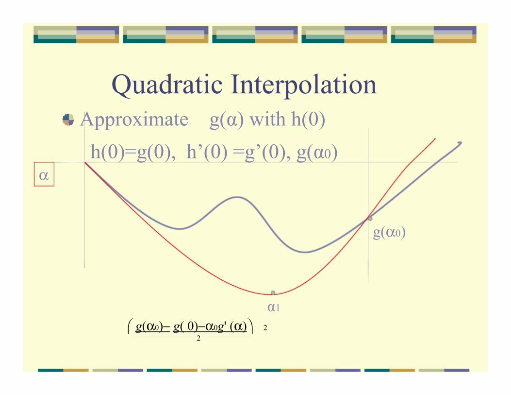
Quadratic Interpolation

Approximate g(α) with h(0)

h(0)=g(0), h’(0) =g’(0), g(α0) α

g(α0)

α1

⎛ g(α0)− g( 0)−α0g' (α)⎞ 2 2

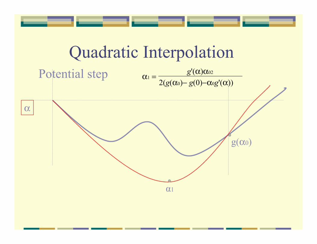
Quadratic Interpolation Potential step

α

α1 = g'(α)α02

2(g(α0)− g(0)−α0g'(α))

g(α0)

α1

⎢b⎥ = α α 2(α −α )⎜ −α03 ⎣ ⎦ ⎝ α1 ⎠⎝g(α0)− g(0)− g'(0)α0 ⎠

2

2 0 1 1 0

Cubic Interpolation

h(α) = aα 3 +bα 2 +αg'(0)+ g(0)

⎡a⎤ 1 ⎛ α0 −α12 ⎞⎛g(α1 )− g(0)− g'(0)α1 ⎞ 3 ⎟⎜ ⎟

−b+ b2 −3ag'(0) 3a α2 =

Cubic Interpolation

3.2.2.2 LINE SEARCH METHODS: OTHER LINE SEARCH PRINCIPLES

Unconstrained optimization methods

xk+1 = xk +! k dk

! k : dk :Step length Search direction

1) Line search

2) Trust-Region algorithms

Quadratic approximation

Influences

Step length computation:

1) Armijo rule:

2) Goldstein rule:

!1" k gkT dk # f (xk +" k dk ) $ f (xk ) # !2" k gk

T dk

0 < !2 <12 < !1 <1

f (xk ) ! f (xk + "m# k dk ) $ !%"m# k&f (xk )T dk

! "(0,1) ! "(0,1/ 2)

! k = "(#f (xk )T dk ) / dk

2

3) Wolfe conditions:

f (xk +! k dk ) " f (xk ) # $! k gkT dk

!f (xk +" k dk )T dk # $gkT dk

0 < ! " # <1

Implementations:

Shanno (1978)

Moré - Thuente (1992-1994)

3.2.2.3 LINE SEARCH METHODS: TAXONOMY OF METHODS

Methods for Unconstrained Optimization

1) Steepest descent (Cauchy, 1847)

dk = !"f (xk )

dk = !"2 f (xk )!1"f (xk )

2) Newton

3) Quasi-Newton (Broyden, 1965; and many others)

dk = Hk!f (xk ) 2 1( )k kH f x −≅ ∇

4) Conjugate Gradient Methods (1952)

dk+1 = !gk+1 + "ksk

sk = xk+1 ! xk

dk ! "#2 f (xk )"1 gk rk = !2 f (xk )dk + gk

!k is known as the conjugate gradient parameter

5) Truncated Newton method (Dembo, et al, 1982)

6) Trust Region methods

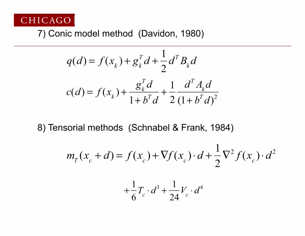
7) Conic model method (Davidon, 1980)

c(d) = f (xk ) +

gkT d

1+ bT d+ 1

2dT Ak d

(1+ bT d)2

q(d) = f (xk ) + gk

T d + 12

dT Bk d

8) Tensorial methods (Schnabel & Frank, 1984)

mT (xc + d) = f (xc ) +!f (xc ) "d + 1

2!2 f (xc ) "d 2

+ 1

6Tc !d

3 + 124

Vc !d4

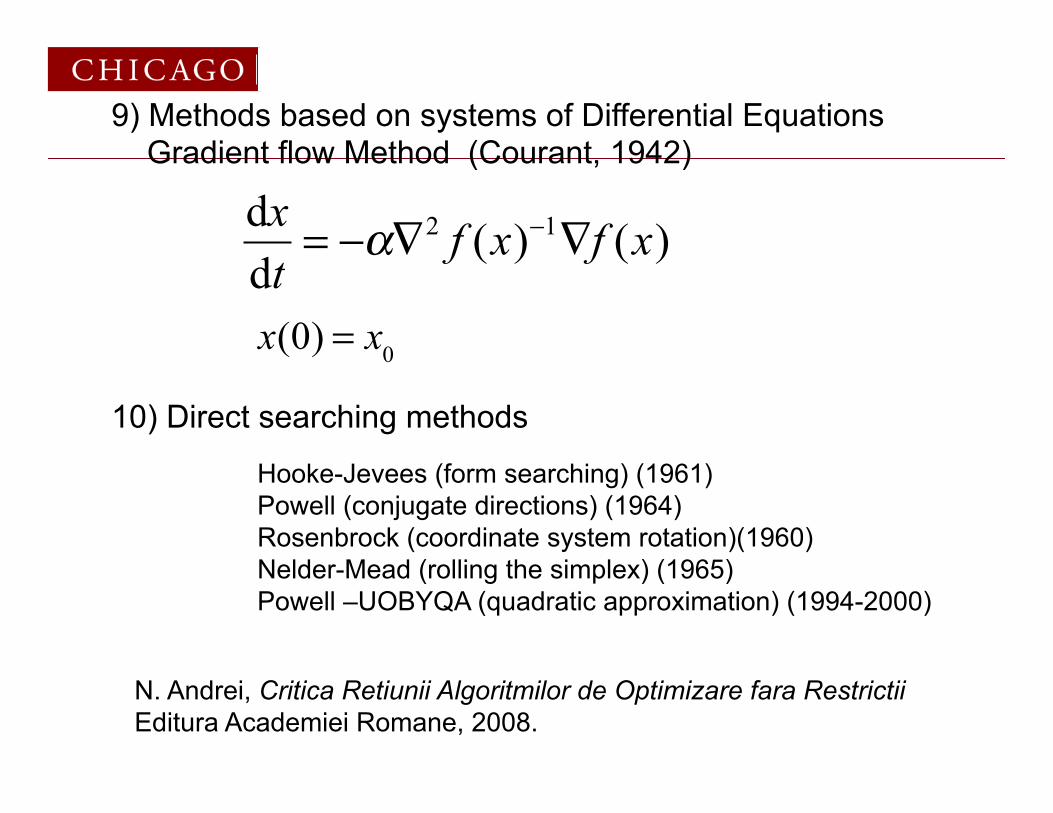
10) Direct searching methods

9) Methods based on systems of Differential Equations Gradient flow Method (Courant, 1942)

dxdt

= !"#2 f (x)!1#f (x)

x(0) = x0

Hooke-Jevees (form searching) (1961) Powell (conjugate directions) (1964) Rosenbrock (coordinate system rotation)(1960) Nelder-Mead (rolling the simplex) (1965) Powell –UOBYQA (quadratic approximation) (1994-2000)

N. Andrei, Critica Retiunii Algoritmilor de Optimizare fara Restrictii Editura Academiei Romane, 2008.

3.3 DEALING WITH INDEFINITE HESSIANS MATRICES

Closest Positive Definite Matrix

•  But Hessian is positive definite (maybe) ONLY at solution!! What do we do?

•  Answer: Perturb the matrix. •  Frobenius NORM •  Closest Positive Definite

Matrix (symmetric A)

A F = aij2

i, j=1

n

! = tr(A*A) = " i2

i=1

n

!

A = AT ! A F = aij2

i, j=1

n

" = tr(A2 ) = #i2

i=1

n

"

Q1TQ1 =Q2

TQ2 ! Q1AQ2 F = A F

A =QDQT A1 =QBQT

B =!i !i " # > 0# !i < #

$%&

'&

Modifying Hessian

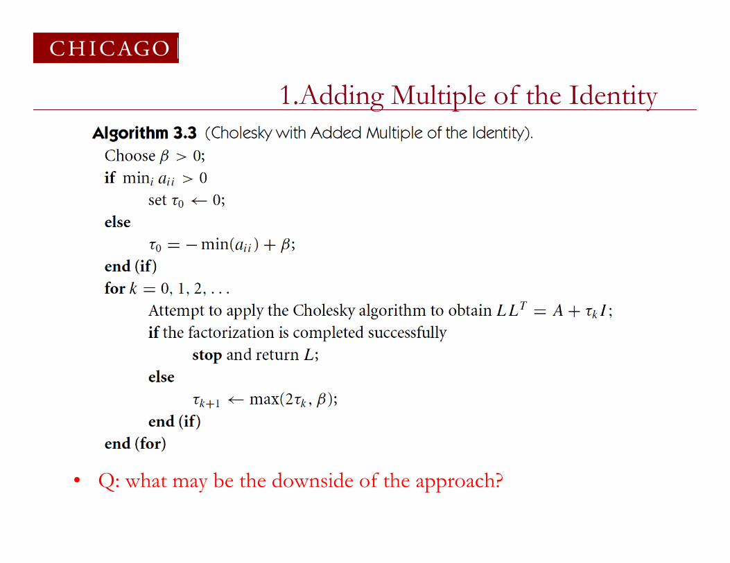
1.Adding Multiple of the Identity

•  Q: what may be the downside of the approach?

2. Modified Cholesky • Ensuring Quality of the Modified Factorization (i.e. entries do not blow up by division to smal l elelments) • AIM:

• Solution: Once a “too small d” is encountered Replace its value by : • Then:

•  Q: Cholesky does not need pivoting. But does it make sense here to NOT pivot?

Bkd = !"f xk( ) # LDLTd = "f xk( )Bk = "xx

2 f xk( ) + Ek

LDL factorization WITH permutation (why?)

•  EXPAND

3. Modified LDLT (maybe most practical to implement ?)

•  What seems to be a practical perturbation to PD that makes it have smallest eigenvalue Delta?

•  Solution: Keep same L,P, modify only the B!

I will ask you to code it with Armijo

3.4 QUASI-NEWTON METHODS

169

3.4 QUASI-NEWTON METHODS: ESSENTIALS

170

Secant Method – Derivation (NLE)

)(xf)f(x - = xx

i

iii ′+1

f(x)

f(xi)

f(xi-1)

xi+2 xi+1 xi X θ

( )[ ]ii xfx ,

1

1)()()(

−

−

−−

=′ii

iii xx

xfxfxf

)()())((

1

11

−

−+ −

−−=

ii

iiiii xfxf

xxxfxx

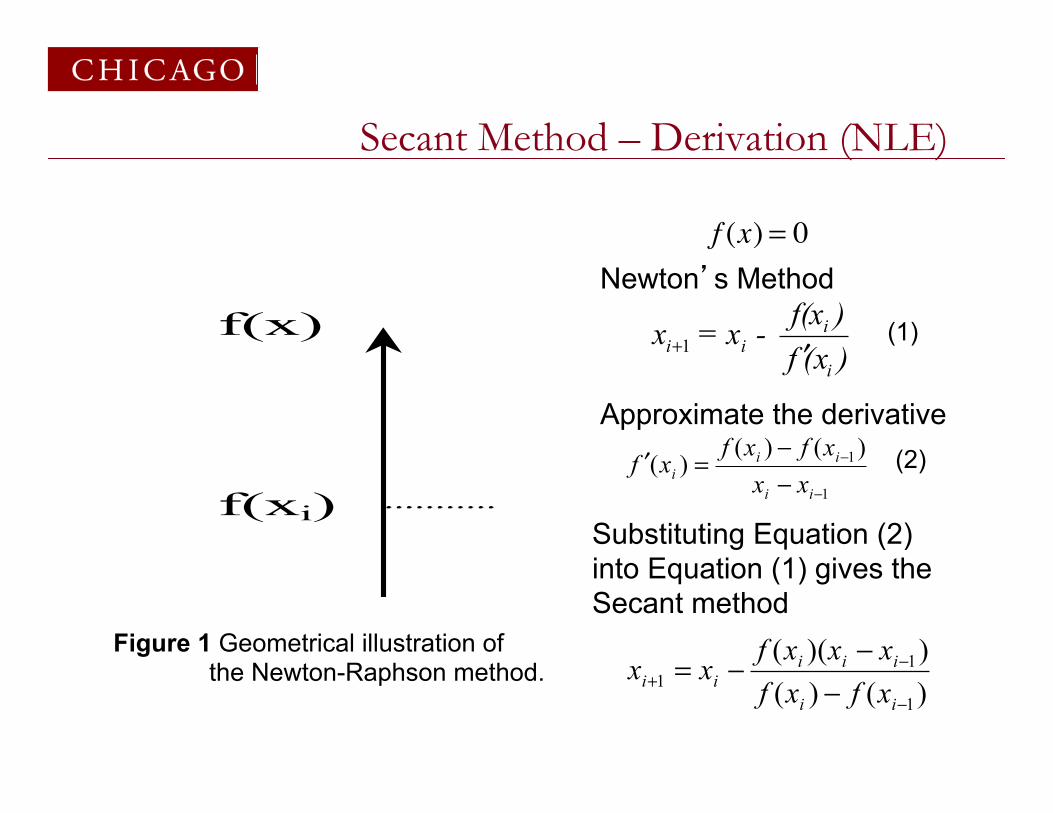
Newton’s Method

Approximate the derivative

Substituting Equation (2) into Equation (1) gives the Secant method

(1)

(2)

Figure 1 Geometrical illustration of the Newton-Raphson method.

f (x) = 0

Secant Method – Derivation

172 )()())((

1

11

−

−+ −

−−=

ii

iiiii xfxf

xxxfxx

The Geometric Similar Triangles

f(x)

f(xi)

f(xi-1)

xi+1 xi-1 xi X

B

C

E D A

11

1

1

)()(

+−

−

+ −=

− ii

i

ii

i

xxxf

xxxf

DEDC

AEAB =

Figure 2 Geometrical representation of the Secant method.

The secant method can also be derived from geometry:

can be written as

On rearranging, the secant method is given as

Multidimensional Secant Condtions.

173

Given two points xk and xk+1 , we define (for an optimization problem) and Further, let pk = xk+1 - xk , then

gk+1 - gk ≈ H(xk) pk If the Hessian is constant, then

gk+1 - gk = H pk which can be rewritten as qk = H pk If the Hessian is constant, then the following condition would hold as well

H-1k+1 qi = pi 0 ≤ i ≤ k

This is called the quasi-Newton condition.

gk = !f xk( ) gk+1 = !f xk+1( )

The Secant Condition

Broyden–Fletcher–Goldfarb–Shanno

174

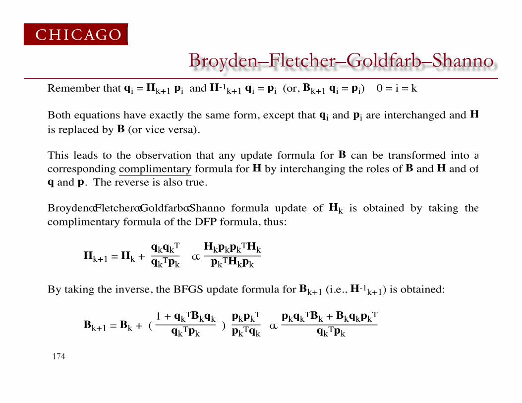
Remember that qi = Hk+1 pi and H-1k+1 qi = pi (or, Bk+1 qi = pi) 0 = i = k

Both equations have exactly the same form, except that qi and pi are interchanged and His replaced by B (or vice versa).

This leads to the observation that any update formula for B can be transformed into acorresponding complimentary formula for H by interchanging the roles of B and H and ofq and p. The reverse is also true.

BroydenœFletcherœGoldfarbœShanno formula update of Hk is obtained by taking thecomplimentary formula of the DFP formula, thus:

Hk+1 = Hk + qkqkT

qkTpk œ

HkpkpkTHkpkTHkpk

By taking the inverse, the BFGS update formula for Bk+1 (i.e., H-1k+1) is obtained:

Bk+1 = Bk + ( 1 + qkTBkqk

qkTpk )

pkpkT

pkTqk œ

pkqkTBk + BkqkpkT

qkTpk

How do BFGS methods work?

Advantage of quasi-Newton

•  Matrix is ALWAYS positive definite, so line search works fine. •  It needs ONLY gradient information. •  It behaves *almost* like Newton in the limit (convergence is

superlinear). •  Optimality is nice, but what you really need is that (1) it needs

only derivatives and (2) it satisfies the secant property and (3) if the original matrix is PSD so is the update. I will ask you to prove them.

•  In its L-BFGS variant it is the workhorse of weather forecast and operational data assimilation in general (a max likelihood procedure, really).

4.1 TRUST REGION FUNDAMENTALS

Trust Region Idea

•  Notations

•  Quadratic Model

•  Order of Quadratic Model (Taylor)

f k = f xk( ) !f k = !f xk( )

mk p( ) = f k + pT gk + 12pT Bk p

f xk + p( ) = f k + pT gk + 12pT!xx

2 f xk + tp( ) p t "[0,1]

mk p( )! f xk + p( ) =O p 2( )O p 2( ) Bk = "xx

2 f xk( )

#

$%

&%

Trust Region Subproblem

minp!Rn

mk p( )subject to p " #k

Called Trust Region Constraint

•  If where then is the solution of the TR subproblem.

•  But the interesting case lies in the opposite situation (since not, why would you need the TR in first place )?

Bk ! 0 and p*k = Bk( )!1

gk ; p*k ! "k pk

Trust Region Geometric Intuition

Example

minx x2 !1( )2

•  Line search started at 0 cannot progress. •  How about the trust-region?

•  Either solution will escape the saddle point --

that is the principle of trust-region.

mind! 2d2; d " #

General approach

•  How do we solve the TR subproblem? •  If (or if we are not obsessed with

stopping at saddle points) we use “dogleg” method. (LS, NLE). Most linear algebra is in computing

•  If fear saddle points, we have to mess around

with eigenvalues and eigenvectors – much harder problem.

Bk ! 0

Bkdk ,U = !gk

Trust Region Management: Parameters

•  The quality of the reduction.

•  Define the acceptance ratio

•  Define the maximum TR size

!k =f xk( )" f xk + pk( )mk 0( )" mk pk( )

Actual Reduction

Predicted Reduction

! " 0, 14

#$%

&'(

!̂; ! " 0, !̂#$ )

TR management

I will ask you to code It with dogleg

What if I cannot solve the TR exactly ?

•  Since it is a hard problem. •  Will this destroy the “Global” convergence behavior? •  Idea: Accept a “sufficient” reduction. •  But, I have no Armijo (or Wolfe, Goldshtein criterion) … •  What do I do? •  Idea? Solve a simple TR problem that creates the yardstick for

acceptance – the Cauchy point.

4.2 THE CAUCHY POINT

The Cauchy Point •  What is an easy model to solve? Linear model

•  Solve TR linear model

•  The Cauchy point.

•  The reduction becomes my yardstick; if trust region has at

least this decrease, I can guarantee “global” convergence (reduction is )

lk p( ) = f k + gk ,T p

pk ,s = argminp!Rn p "#k lk p( )

! k = argmin!"R ! pk ,s #$k mk ! pk ,s( )

pk ,c = ! k pk ,s; xk ,c = xk + pk ,c

m(0)! m pk ,c( )

O gk2( )

Cauchy Point Solution

•  First, solution of the linear problem is

•  Then, it immediately follows that

pks = ! "k

gkgk

! k =

1 gkT Bkgk " 0

mingk

3

gkT Bkgk( )#k

,1$

%&

'

() otherwise

*

+,,

-,,

Dogleg Methods: Improve CP

•  If Cauchy point is on the boundary I have a lot of decrease and I accept it (e.g if )

•  If Cauchy point is interior,

•  Take now “Newton” step (note, B need not be pd, all I need is nonsingular).

gk ,T Bkgk > 0; pk ,c = !

gk2

gk ,T Bkgk g

k

gk ,T Bkgk ! 0;

pB = !Bk!1gk

Dogleg Method Continued

•  Define dogleg path

•  The dogleg point:

•  It is obtained by solving 2 quadratics. •  Sufficiently close to the solution it allows me to choose the

Newton step, and thus quadratic convergence.

!p !( ) =! pk ,c ! "1

pk ,c + ! #1( ) pB # pk ,c( ) 1" ! " 2

$%&

'&

! = 2

!p !D( ); !D = argmin! ; !p !( ) "#k

mk !p !( )( )

I will ask you to code it with TR

Dogleg Method: Theory

Global Convergence of CP Methods

Numerical comparison between methods

•  What is a fair comparison between methods? •  Probably : starting from same point 1) number of function evaluations

and 2) number of linear systems (the rest depends too much on the hardware and software platform). I will ask you to do this.

•  Trust region tends to use fewer function evaluations (the modern preferred metric; ) than line search .

•  Also dogleg does not force positive definite matrix, so it has fewer chances of stopping at a saddle point, (but it is not guaranteed either).

4.3 GENERAL CASE: SOLVING THE ACTUAL TR PROBLEM (DOGLEG DOES NOT QUITE DO IT)

Trust Region Equation

Theory of Trust Region Problem

Global convergence away from saddle point

Fast Local Convergence

How do we solve the subproblem?

•  Very sophisticated approach based on theorem on structure of TR solution, eigenvalue analysis and/or an “inner” Newton iteration.

•  Foundation: Find Solution for

How do I find such a solution?

TR problem has a solution

!

Practical (INCOMPLETE) algorithm

It generally gives a machine precision solution in 2-3 iterations (Cholesky)

The Hard Case

qjT g = 0

! = "!1 # p =qjT g

! j " !1j:! j $!1% qj

p !( ) = qjT g

" j # "1j:" j $"1% qj + !q1

!" p "( ) = #k

If double root, things continue to be complicated …

Summary and Comparisons

•  Line search problems have easier subproblems (if we modify Cholesky).

•  But they cannot be guaranteed to converge to a point with positive semidefinite Hessian.

•  Trust-region problems can, at the cost of solving a complicated subproblem.

•  Dogleg methods leave “between” these two situations.