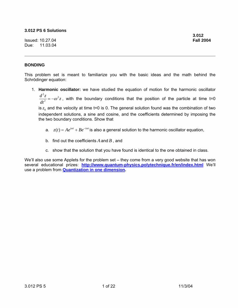
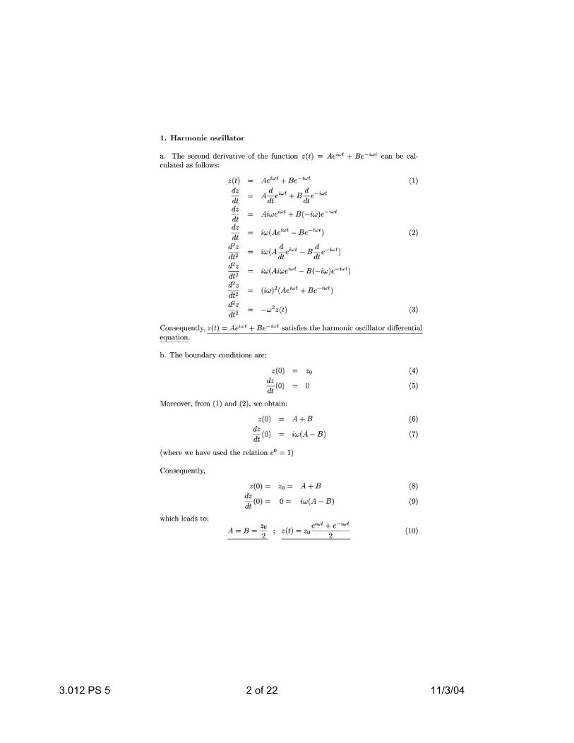
3.012 PS 5 1 of 22 11/3/04

3.012 PS 6 Solutions 3.012 Issued: 10.27.04 Fall 2004 Due: 11.03.04

BONDING This problem set is meant to familiarize you with the basic ideas and the math behind the Schrödinger equation:

1. Harmonic oscillator: we have studied the equation of motion for the harmonic oscillator 2

22

d z zdt

ω= − , with the boundary conditions that the position of the particle at time t=0

is 0z and the velocity at time t=0 is 0. The general solution found was the combination of two independent solutions, a sine and cosine, and the coefficients determined by imposing the the two boundary conditions. Show that

a. ( ) i t i tz t Ae Beω ω−= + is also a general solution to the harmonic oscillator equation,

b. find out the coefficients A and B , and

c. show that the solution that you have found is identical to the one obtained in class.

We’ll also use some Applets for the problem set – they come from a very good website that has won several educational prizes: http://www.quantum-physics.polytechnique.fr/en/index.html We’ll use a problem from Quantization in one dimension.

3.012 PS 5 2 of 22 11/3/04

3.012 PS 5 3 of 22 11/3/04

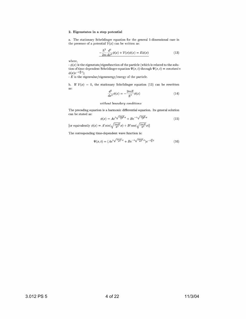
2. Eigenstates in a step potential: Here our potential is represented by a green line, and it is 0 on the right side of the picture, and it is constant and positive (=V0) on the left side of the picture. With the mouse, you can slide the trial value of the energy E (in red) that appears in the Schrödinger equation from below zero to above V0. The applet instantaneously tries to calculate a function (in yellow/white) that solves the Schrödinger equation for the chosen energy E. It turns out that for any energy E greater than 0 the applet finds a well-behaved eigenfunction – so we have a continuous spectrum of eigenvalues (i.e. set of solutions), each of them with its corresponding eigenfunction.

• Write the Schrödinger equation for the general 1-dimensional case in the presence of a potential.

• Discuss its solutions in the case of the potential being zero everywhere – is there a continuous or discrete spectrum of eigenvalues ?

• Discuss the eigenfunctions of the problem in the applet, where the potential V(x) is 0 for x > 0, and is equal to V0 for x < 0. What happens when we look for a solution corresponding to an eigenvalue above V0 ? What if we choose an energy below V0, but above 0 ?

3.012 PS 5 4 of 22 11/3/04

3.012 PS 5 5 of 22 11/3/04

3.012 PS 5 6 of 22 11/3/04

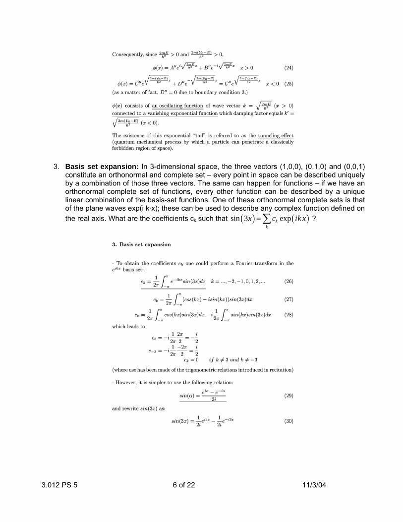
3. Basis set expansion: In 3-dimensional space, the three vectors (1,0,0), (0,1,0) and (0,0,1) constitute an orthonormal and complete set – every point in space can be described uniquely by a combination of those three vectors. The same can happen for functions – if we have an orthonormal complete set of functions, every other function can be described by a unique linear combination of the basis-set functions. One of these orthonormal complete sets is that of the plane waves exp(i k·x); these can be used to describe any complex function defined on the real axis. What are the coefficients ck such that ( ) ( )sin 3 expk

kx c ik x= ∑ ?

3.012 PS 5 7 of 22 11/3/04

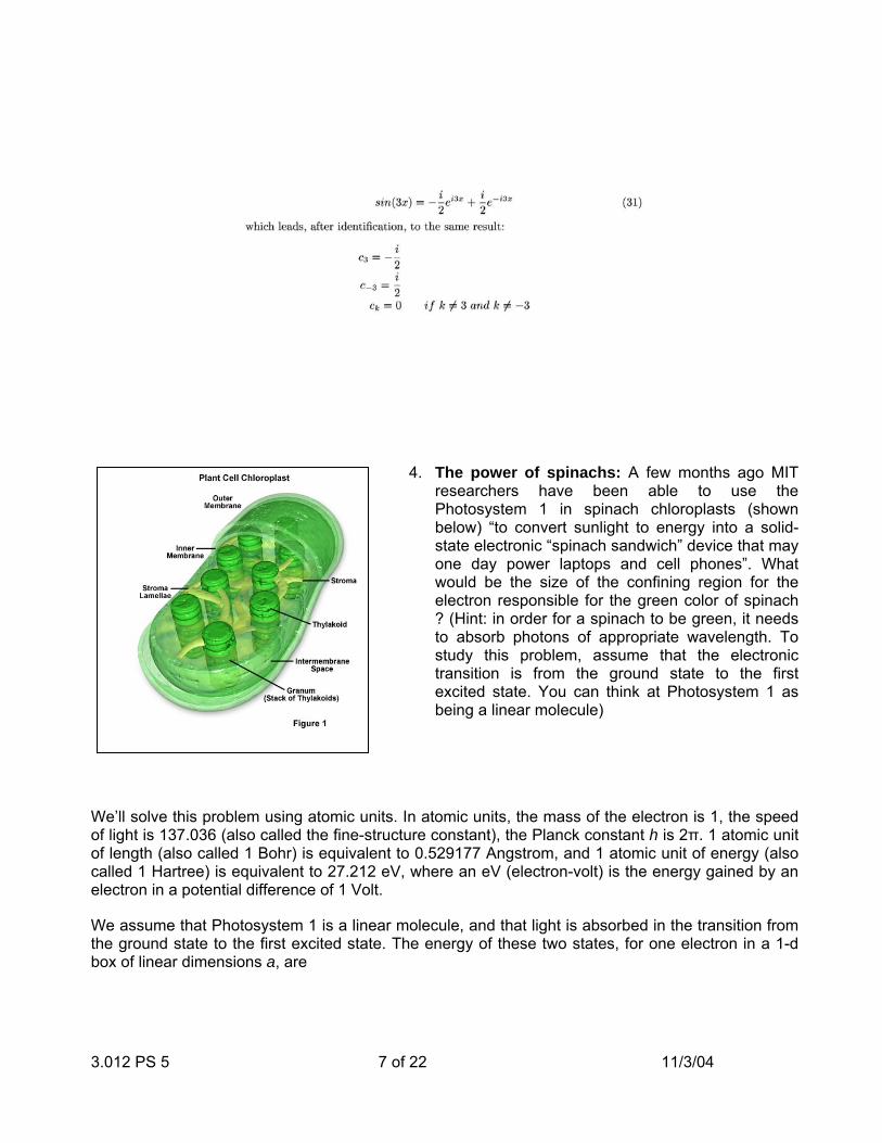
4. The power of spinachs: A few months ago MIT researchers have been able to use the Photosystem 1 in spinach chloroplasts (shown below) “to convert sunlight to energy into a solid-state electronic “spinach sandwich” device that may one day power laptops and cell phones”. What would be the size of the confining region for the electron responsible for the green color of spinach ? (Hint: in order for a spinach to be green, it needs to absorb photons of appropriate wavelength. To study this problem, assume that the electronic transition is from the ground state to the first excited state. You can think at Photosystem 1 as being a linear molecule)

We’ll solve this problem using atomic units. In atomic units, the mass of the electron is 1, the speed of light is 137.036 (also called the fine-structure constant), the Planck constant h is 2π. 1 atomic unit of length (also called 1 Bohr) is equivalent to 0.529177 Angstrom, and 1 atomic unit of energy (also called 1 Hartree) is equivalent to 27.212 eV, where an eV (electron-volt) is the energy gained by an electron in a potential difference of 1 Volt.

We assume that Photosystem 1 is a linear molecule, and that light is absorbed in the transition from the ground state to the first excited state. The energy of these two states, for one electron in a 1-d box of linear dimensions a, are

3.012 PS 5 8 of 22 11/3/04

( )22 2 2

2 2

2 (in atomic units)

8 8h n nEm a a

π= = , where a in the last term is meant to be expressed in Bohr.

The energy difference between the ground (n=1) and the first excited state (n=2) need to be equal to

the energy of the absorbed electromagnetic radiation 2(in atomic units) hcE π

λ λ= = . Thus, we

obtain the relation( ) ( )2 2

2 2

2 24 1 2 (137.036) -8 8a aπ π π

λ= , or

34(137.036)

a π λ= . For a typical

wavelength in the blue region (400 nm, or roughly 7500 Bohr) we obtain a box of dimension 11.35 Bohr, or ~ 6 Å (Angstrom, 1 Å=10-10 m).

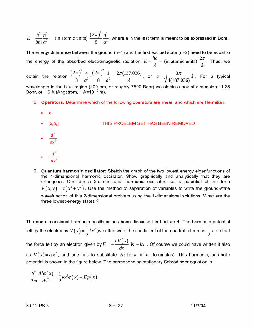
5. Operators: Determine which of the following operators are linear, and which are Hermitian:

• x

• [x,px] THIS PROBLEM SET HAS BEEN REMOVED

• 2

2

ddx

• i2

2

ddx

6. Quantum harmonic oscillator: Sketch the graph of the two lowest energy eigenfunctions of the 1-dimensional harmonic oscillator. Show graphically and analytically that they are orthogonal. Consider a 2-dimensional harmonic oscillator, i.e. a potential of the form

( ) ( )2 2,V x y x yα= + . Use the method of separation of variables to write the ground-state wavefunction of this 2-dimensional problem using the 1-dimensional solutions. What are the three lowest-energy states ?

The one-dimensional harmonic oscillator has been discussed in Lecture 4. The harmonic potential

felt by the electron is ( ) 212

V x kx= (we often write the coefficient of the quadratic term as 12

k so that

the force felt by an electron given by( ) is

dV xF kx

dx= − − . Of course we could have written it also

as ( ) 2V x xα= , and one has to substitute 2 for kα in all forumulas). This harmonic, parabolic potential is shown in the figure below. The corresponding stationary Schrödinger equation is

( ) ( ) ( )22

22

12 2

d xkx x E x

m dxϕ

ϕ ϕ− + =h

3.012 PS 5 9 of 22 11/3/04

The only allowed “eigenvalues” of the energy E for which the above equation has a proper solution

are given by 12

E nω ⎛ ⎞= +⎜ ⎟⎝ ⎠

h , where the quantum number n can take any integer value 0, 1, 2, …. .

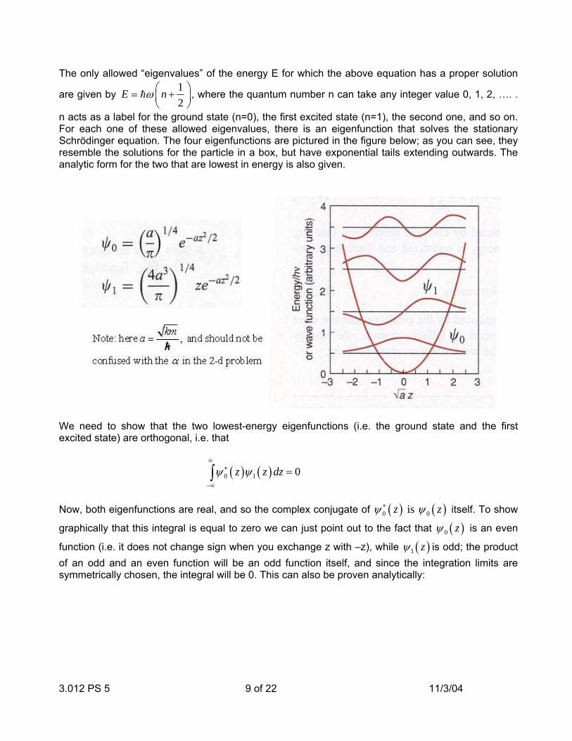
n acts as a label for the ground state (n=0), the first excited state (n=1), the second one, and so on. For each one of these allowed eigenvalues, there is an eigenfunction that solves the stationary Schrödinger equation. The four eigenfunctions are pictured in the figure below; as you can see, they resemble the solutions for the particle in a box, but have exponential tails extending outwards. The analytic form for the two that are lowest in energy is also given.

We need to show that the two lowest-energy eigenfunctions (i.e. the ground state and the first excited state) are orthogonal, i.e. that

( ) ( )0 1 0z z dzψ ψ∞

∗

−∞

=∫

Now, both eigenfunctions are real, and so the complex conjugate of ( ) ( )0 0 is z zψ ψ∗ itself. To show

graphically that this integral is equal to zero we can just point out to the fact that ( )0 zψ is an even

function (i.e. it does not change sign when you exchange z with –z), while ( )1 zψ is odd; the product of an odd and an even function will be an odd function itself, and since the integration limits are symmetrically chosen, the integral will be 0. This can also be proven analytically:

3.012 PS 5 10 of 22 11/3/04

( ) ( ) ( ) ( ) ( ) ( ) ( ) ( ) ( ) ( )

( ) ( ) ( ) ( ) ( ) ( ) ( ) ( )

0 0

0 1 0 1 0 1 0 1 0 10 0

0

0 1 0 0 1 00 0 0

( )

( ) 0

z z dz z z dz z z dz t t d t z z dz

t t dt z z dz t t d t z z dz

ψ ψ ψ ψ ψ ψ ψ ψ ψ ψ

ψ ψ ψ ψ ψ ψ ψ ψ

∞ ∞ ∞∗

−∞ −∞ −∞

∞ ∞ ∞

−∞

= + = − − − + =

+ = − + =

∫ ∫ ∫ ∫ ∫

∫ ∫ ∫ ∫

(we have removed the complex-conjugate symbol, since the functions are real, and we have exploited the fact that ( ) ( ) ( ) ( )0 0 1 1 and t t t tψ ψ ψ ψ= − = − − ).

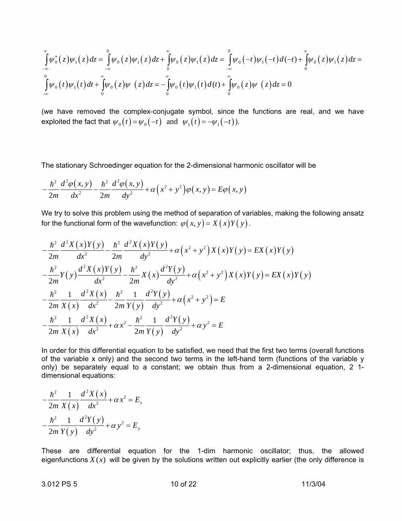
The stationary Schroedinger equation for the 2-dimensional harmonic oscillator will be

( ) ( ) ( ) ( ) ( )2 22 2

2 22 2

, ,, ,

2 2d x y d x y

x y x y E x ym dx m dy

ϕ ϕα ϕ ϕ− − + + =

h h

We try to solve this problem using the method of separation of variables, making the following ansatz for the functional form of the wavefunction: ( ) ( ) ( ),x y X x Y yϕ = .

( ) ( ) ( ) ( ) ( ) ( ) ( ) ( ) ( )

( ) ( ) ( ) ( ) ( ) ( ) ( ) ( ) ( ) ( )

( )( )

( )( ) ( )

( )( )

( )( )

2 22 22 2

2 2

2 22 22 2

2 2

2 22 22 2

2 2

2 22 22 2

2 2

2 2

2 2

1 12 2

1 12 2

d X x Y y d X x Y yx y X x Y y EX x Y y

m dx m dyd X x Y y d Y y

Y y X x x y X x Y y EX x Y ym dx m dy

d X x d Y yx y E

m X x dx m Y y dy

d X x d Y yx y E

m X x dx m Y y dy

α

α

α

α α

− − + + =

− − + + =

− − + + =

− + − + =

h h

h h

h h

h h

In order for this differential equation to be satisfied, we need that the first two terms (overall functions of the variable x only) and the second two terms in the left-hand term (functions of the variable y only) be separately equal to a constant; we obtain thus from a 2-dimensional equation, 2 1-dimensional equations:

( )( )

( )( )

222

2

222

2

12

12

x

y

d X xx E

m X x dx

d Y yy E

m Y y dy

α

α

− + =

− + =

h

h

These are differential equation for the 1-dim harmonic oscillator; thus, the allowed eigenfunctions ( )X x will be given by the solutions written out explicitly earlier (the only difference is

3.012 PS 5 11 of 22 11/3/04

that they will be functions of x, not functions of z…); same for ( )Y y .

( ) ( )Given that x,y is ( )X x Y yϕ , the ground-state wavefunction for the two-dimensional problem will

be given by ( )2 2

x,y exp2 2x yA a aϕ

⎛ ⎞⎛ ⎞= − −⎜ ⎟⎜ ⎟

⎝ ⎠⎝ ⎠ , where

2 is ma αh

, and so on. The three lowest-

energy eigenvalues will be 1 1 ,2 2

E l mω ⎛ ⎞⎛ ⎞= + +⎜ ⎟⎜ ⎟⎝ ⎠⎝ ⎠

h with l=0 and m=0, and then with l=1, m=0 or l=0

and m=1.

3.012 PS 5 12 of 22 11/3/04

THERMODYNAMICS

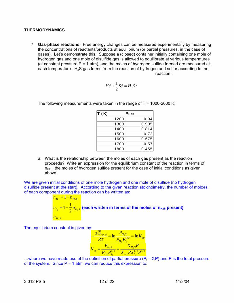
7. Gas-phase reactions. Free energy changes can be measured experimentally by measuring the concentrations of reactants/products at equilibrium (or partial pressures, in the case of gases). Let’s demonstrate this. Suppose a (closed) container initially containing one mole of hydrogen gas and one mole of disulfide gas is allowed to equilibrate at various temperatures (at constant pressure P = 1 atm), and the moles of hydrogen sulfide formed are measured at each temperature. H2S gas forms from the reaction of hydrogen and sulfur according to the

reaction:

The following measurements were taken in the range of T = 1000-2000 K:

T (K) nH2S

1200 0.941300 0.9051400 0.8141500 0.721600 0.6751700 0.571800 0.455

a. What is the relationship between the moles of each gas present as the reaction proceeds? Write an expression for the equilibrium constant of the reaction in terms of nH2S, the moles of hydrogen sulfide present for the case of initial conditions as given above.

We are given initial conditions of one mole hydrogen and one mole of disulfide (no hydrogen disulfide present at the start). According to the given reaction stoichoimetry, the number of moloes of each component during the reaction can be written as:

nH2=1− nH2S

nS2=1−

12

nH2S

nH2S

(each written in terms of the moles of nH2S present)

The equilibrium constant is given by:

−∆G rxn,o

RT= ln

PH2S

PH2PS2

1/ 2 = lnKeq

Keq =PH2S

PH2PS2

1/ 2 =X H2SP

X H2PXS2

1/ 2P1/ 2

…where we have made use of the definition of partial pressure (Pi = XiP) and P is the total pressure of the system. Since P = 1 atm, we can reduce this expression to:

ggg SHSH 222 21

=+

3.012 PS 5 13 of 22 11/3/04

Keq =X H2S

X H2XS2

1/ 2 =nH2Sntotal

1/ 2

nH2nS2

1/ 2 =nH2S( )1− nH2S +1−

12

nH2S + nH2S

⎛ ⎝ ⎜

⎞ ⎠ ⎟

1/ 2

1− nH2S( )1−12

nH2S

⎛ ⎝ ⎜

⎞ ⎠ ⎟

1/ 2 =nH2S( ) 2 −

12

nH2S

⎛ ⎝ ⎜

⎞ ⎠ ⎟

1/ 2

1− nH2S( )1−12

nH2S

⎛ ⎝ ⎜

⎞ ⎠ ⎟

1/ 2

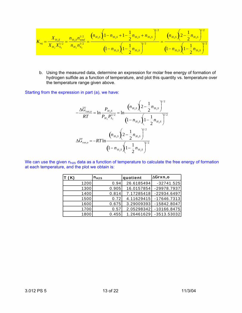
b. Using the measured data, determine an expression for molar free energy of formation of hydrogen sulfide as a function of temperature, and plot this quantity vs. temperature over the temperature range given above.

Starting from the expression in part (a), we have:

−∆G rxn,o

RT= ln

PH2S

PH2PS2

1/ 2 = lnnH2S( ) 2 −

12

nH2S

⎛ ⎝ ⎜

⎞ ⎠ ⎟

1/ 2

1− nH2S( )1−12

nH2S⎛ ⎝ ⎜

⎞ ⎠ ⎟

1/ 2

∆G rxn,o = −RT lnnH2S( ) 2 −

12

nH2S

⎛ ⎝ ⎜

⎞ ⎠ ⎟

1/ 2

1− nH2S( )1−12

nH2S

⎛ ⎝ ⎜

⎞ ⎠ ⎟

1/ 2

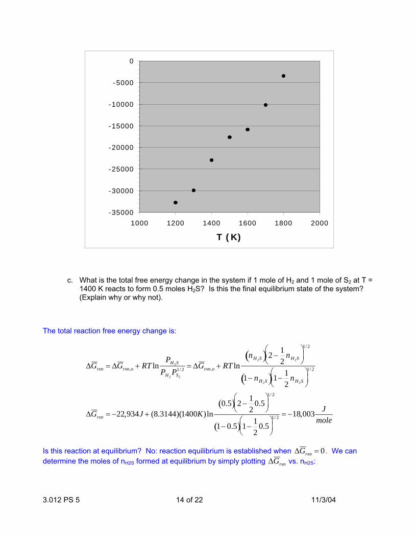
We can use the given nH2S data as a function of temperature to calculate the free energy of formation at each temperature, and the plot we obtain is:

T (K) nH2S quotient ∆Grxn,o

1200 0.94 26.6185494 -32741.5251300 0.905 16.0157854 -29978.79371400 0.814 7.17285418 -22934.64971500 0.72 4.11629415 -17646.73131600 0.675 3.29009393 -15842.80471700 0.57 2.05298342 -10166.84751800 0.455 1.26461629 -3513.53032

3.012 PS 5 14 of 22 11/3/04

-35000

-30000

-25000

-20000

-15000

-10000

-5000

0

1000 1200 1400 1600 1800 2000

T (K)

c. What is the total free energy change in the system if 1 mole of H2 and 1 mole of S2 at T = 1400 K reacts to form 0.5 moles H2S? Is this the final equilibrium state of the system? (Explain why or why not).

The total reaction free energy change is:

∆G rxn = ∆G rxn,o + RT lnPH2S

PH2PS2

1/ 2 = ∆G rxn,o + RT lnnH2S( ) 2 −

12

nH2S

⎛ ⎝ ⎜

⎞ ⎠ ⎟

1/ 2

1− nH2S( )1−12

nH2S⎛ ⎝ ⎜

⎞ ⎠ ⎟

1/ 2

∆G rxn = −22,934J + (8.3144)(1400K)ln0.5( ) 2 −

12

0.5⎛ ⎝ ⎜

⎞ ⎠ ⎟

1/ 2

1− 0.5( ) 1−12

0.5⎛ ⎝ ⎜

⎞ ⎠ ⎟

1/ 2 = −18,003 Jmole

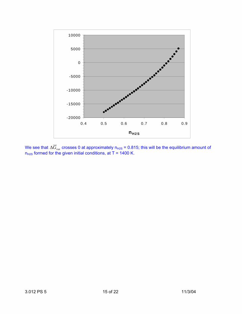
Is this reaction at equilibrium? No: reaction equilibrium is established when ∆G rxn = 0 . We can determine the moles of nH2S formed at equilibrium by simply plotting ∆G rxn vs. nH2S:

3.012 PS 5 15 of 22 11/3/04

-20000

-15000

-10000

-5000

0

5000

10000

0.4 0.5 0.6 0.7 0.8 0.9

nH2S

We see that ∆G rxn crosses 0 at approximately nH2S = 0.815; this will be the equilibrium amount of nH2S formed for the given initial conditions, at T = 1400 K.

3.012 PS 5 16 of 22 11/3/04

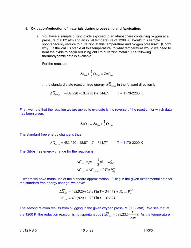
8. Oxidation/reduction of materials during processing and fabrication.

a. You have a sample of zinc oxide exposed to an atmosphere containing oxygen at a pressure of 0.02 atm and an initial temperature of 1200 K. Would this sample spontaneously reduce to pure zinc at this temperature and oxygen pressure? (Show why). If the ZnO is stable at this temperature, to what temperature would we need to heat the oxide to begin reducing ZnO to pure zinc metal? The following thermodynamic data is available:

For the reaction:

Zn(s) +12

O2(g ) = ZnO(s)

…the standard state reaction free energy ∆G rxn,o in the forward direction is:

∆G rxn,o = −482,920 −18.8T lnT + 344.7T T = 1170-2200 K

First, we note that the reaction we are asked to evaluate is the reverse of the reaction for which data has been given:

ZnO(s) = Zn(s) +12

O2(g )

The standard free energy change is thus:

∆G rxn,o = 482,920 +18.8T lnT − 344.7T T = 1170-2200 K The Gibbs free energy change for the reaction is:

∆G rxn = µZng +

12

µO2

g − µZnOg

∆G rxn = ∆G rxn,o + RT lnPO2

1/ 2

…where we have made use of the standard approximation. Filling in the given experimental data for the standard free energy change, we have:

∆G rxn = 482,920 +18.8T lnT − 344.7T + RT ln PO2

1/ 2

∆G rxn = 482,920 +18.8T lnT − 377.2T

The second relation results from plugging in the given oxygen pressure (0.02 atm). We see that at

the 1200 K, the reduction reaction is not spontaneous (∆G rxn = 598,232 Jmole

). As the temperature

3.012 PS 5 17 of 22 11/3/04

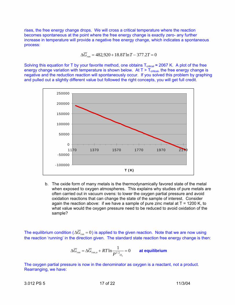
rises, the free energy change drops. We will cross a critical temperature where the reaction becomes spontaneous at the point where the free energy change is exactly zero- any further increase in temperature will provide a negative free energy change, which indicates a spontaneous process:

∆G rxn = 482,920 +18.8T lnT − 377.2T = 0 Solving this equation for T by your favorite method, one obtains Tcritical ≈ 2067 K. A plot of the free energy change variation with temperature is shown below. At T > Tcritical, the free energy change is negative and the reduction reaction will spontaneously occur. If you solved this problem by graphing and pulled out a slightly different value but followed the right concepts, you will get full credit.

-100000

-50000

0

50000

100000

150000

200000

250000

1170 1370 1570 1770 1970 2170

T (K)

b. The oxide form of many metals is the thermodynamically favored state of the metal when exposed to oxygen atmospheres. This explains why studies of pure metals are often carried out in vacuum ovens: to lower the oxygen partial pressure and avoid oxidation reactions that can change the state of the sample of interest. Consider again the reaction above: if we have a sample of pure zinc metal at T = 1200 K, to what value would the oxygen pressure need to be reduced to avoid oxidation of the sample?

The equilibrium condition ( ∆G rxn = 0 ) is applied to the given reaction. Note that we are now using the reaction ‘running’ in the direction given. The standard state reaction free energy change is then:

∆G rxn = ∆G rxn,o + RT ln 1P1/ 2

O2

= 0 at equilibrium

The oxygen partial pressure is now in the denominator as oxygen is a reactant, not a product. Rearranging, we have:

3.012 PS 5 18 of 22 11/3/04

∆G rxn,o = −RT ln 1P1/ 2

O2

We can fill in the given standard state free energy change data and back out the partial pressure of oxygen present at equilibrium for the oxidation reaction:

∆G rxn,o = −482,920 −18.8T lnT + 344.7T = −RT ln 1P1/ 2

O2

∆G rxn,o = −229,232 Jmole

@T =1200K

Thus PO2 = 1.0255x10-5 atm at equilibrium, and we must have a pressure smaller than this to avoid oxidation of the Zinc. Recall that oxygen makes up ~20% of the natural atmosphere, which will

strongly favor the reaction ( RT ln 1P1/ 2

O2

=16,057 Jmole

, much smaller than the standard state

reaction free energy change).

3.012 PS 5 19 of 22 11/3/04

9. Electrochemical cells. A Daniell electrochemical cell is prepared with the structure:

PbI PbCl2(aq )II Hg2Cl2(aq )

III HgIV

…where the vertical lines designate separations between the phases I-IV of the cell; the double line represents the membrane separating the two aqueous electrolyte solutions (phases II and III). The EMF of the cell is 0.5357 volts at 25°C.

a. What are the half-cell reactions for this battery?

This battery is very similar to the example discussed in lecture. At the anode, we have:

Pb(s)I = Pb(aq )

++( )II+ 2 e −( )I

At the opposite electrode:

2 Hg(aq )+( )III

+ 2 e −( )IV = 2Hg(s)IV

b. What is the maximum amount of work that can be extracted from this battery at 25°C?

The maximum work is related to the free energy change per mole of reaction in the battery:

dwmax = −dGwmax = −∆G rxn

The reaction free energy change is in turn related to the battery’s EMF by the Nernst equation:

∆φ = ε = −∆G rxn

2F=

wmax

2F

wmax = 2Fε = 2 96,485 Cmole

⎛ ⎝ ⎜

⎞ ⎠ ⎟ 0.5357volts( )=103,374 J

mole

Note that capital ‘F’ throughout this problem solution refers to the Faraday constant, not the Helmholtz free energy.

c. The mercury electrode in the cell is replaced by an Hg-X alloy in which XHg = 0.3 and X is an inert component that does not participate in the cell reactions. The EMF of the cell is found to increase by 0.0089 volts. Calculate the activity and activity coefficient of Hg in the alloy at 25°C.

3.012 PS 5 20 of 22 11/3/04

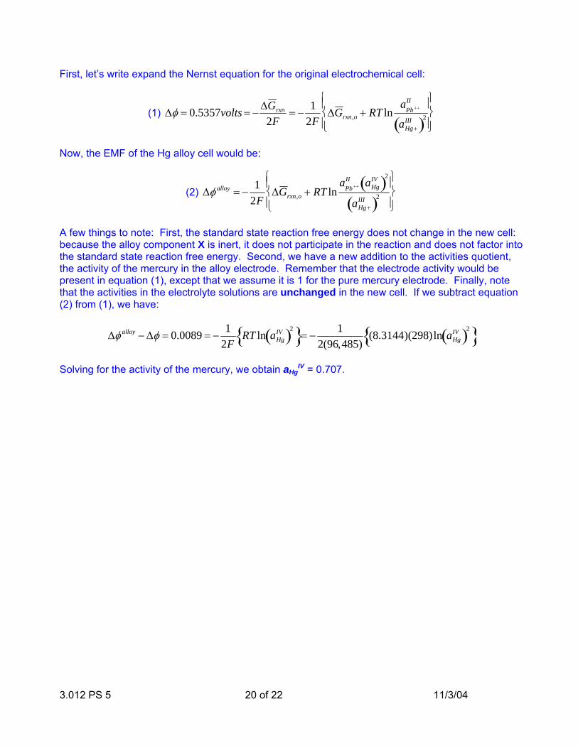
First, let’s write expand the Nernst equation for the original electrochemical cell:

(1) ∆φ = 0.5357volts = −∆G rxn

2F= −

12F

∆G rxn,o + RT lna

Pb ++II

aHg +III( )2

⎧ ⎨ ⎪

⎩ ⎪

⎫ ⎬ ⎪

⎭ ⎪

Now, the EMF of the Hg alloy cell would be:

(2) ∆φ alloy = −1

2F∆G rxn,o + RT ln

aPb ++II aHg

IV( )2

aHg +III( )2

⎧ ⎨ ⎪

⎩ ⎪

⎫ ⎬ ⎪

⎭ ⎪

A few things to note: First, the standard state reaction free energy does not change in the new cell: because the alloy component X is inert, it does not participate in the reaction and does not factor into the standard state reaction free energy. Second, we have a new addition to the activities quotient, the activity of the mercury in the alloy electrode. Remember that the electrode activity would be present in equation (1), except that we assume it is 1 for the pure mercury electrode. Finally, note that the activities in the electrolyte solutions are unchanged in the new cell. If we subtract equation (2) from (1), we have:

∆φ alloy − ∆φ = 0.0089 = −1

2FRT ln aHg

IV( )2{ }= −1

2(96,485)(8.3144)(298)ln aHg

IV( )2{ }

Solving for the activity of the mercury, we obtain aHg

IV = 0.707.

3.012 PS 5 21 of 22 11/3/04

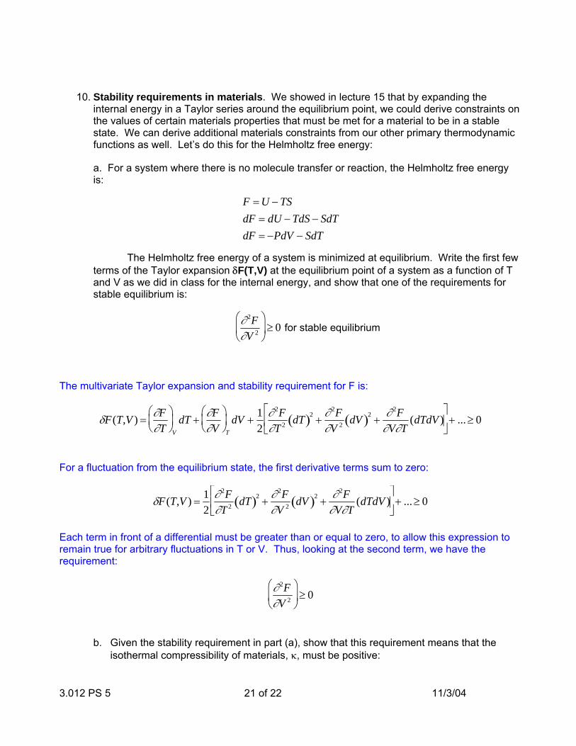
10. Stability requirements in materials. We showed in lecture 15 that by expanding the internal energy in a Taylor series around the equilibrium point, we could derive constraints on the values of certain materials properties that must be met for a material to be in a stable state. We can derive additional materials constraints from our other primary thermodynamic functions as well. Let’s do this for the Helmholtz free energy:

a. For a system where there is no molecule transfer or reaction, the Helmholtz free energy is:

F = U − TSdF = dU − TdS − SdTdF = −PdV − SdT

The Helmholtz free energy of a system is minimized at equilibrium. Write the first few terms of the Taylor expansion δF(T,V) at the equilibrium point of a system as a function of T and V as we did in class for the internal energy, and show that one of the requirements for stable equilibrium is:

∂ 2F∂V 2

⎛

⎝ ⎜

⎞

⎠ ⎟ ≥ 0 for stable equilibrium

The multivariate Taylor expansion and stability requirement for F is:

δF(T,V ) =∂F∂T

⎛ ⎝ ⎜

⎞ ⎠ ⎟

V

dT +∂F∂V

⎛ ⎝ ⎜

⎞ ⎠ ⎟

T

dV +12

∂ 2F∂T 2 dT( )2 +

∂ 2F∂V 2 dV( )2 +

∂ 2F∂V∂T

(dTdV )⎡

⎣ ⎢

⎤

⎦ ⎥ + ...≥ 0

For a fluctuation from the equilibrium state, the first derivative terms sum to zero:

δF(T,V ) =12

∂ 2F∂T 2 dT( )2 +

∂ 2F∂V 2 dV( )2 +

∂ 2F∂V∂T

(dTdV )⎡

⎣ ⎢

⎤

⎦ ⎥ + ...≥ 0

Each term in front of a differential must be greater than or equal to zero, to allow this expression to remain true for arbitrary fluctuations in T or V. Thus, looking at the second term, we have the requirement:

∂ 2F∂V 2

⎛

⎝ ⎜

⎞

⎠ ⎟ ≥ 0

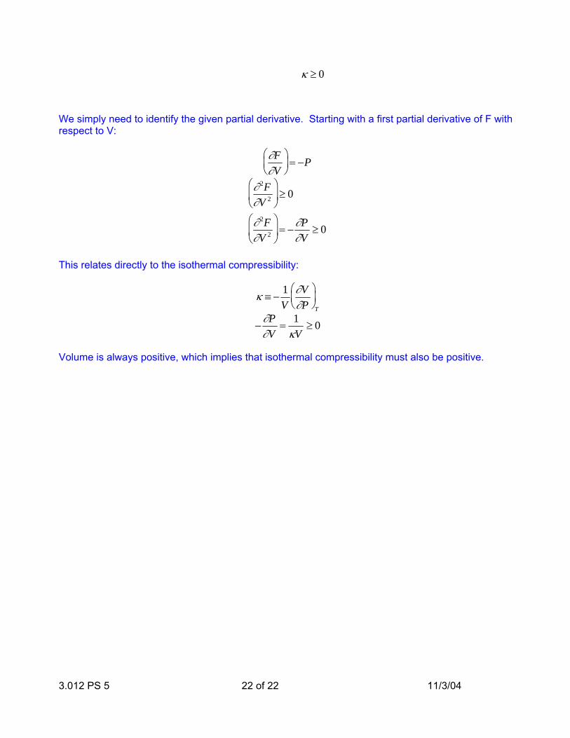
b. Given the stability requirement in part (a), show that this requirement means that the isothermal compressibility of materials, κ, must be positive:

3.012 PS 5 22 of 22 11/3/04

κ ≥ 0

We simply need to identify the given partial derivative. Starting with a first partial derivative of F with respect to V:

∂F∂V

⎛ ⎝ ⎜

⎞ ⎠ ⎟ = −P

∂ 2F∂V 2

⎛

⎝ ⎜

⎞

⎠ ⎟ ≥ 0

∂ 2F∂V 2

⎛

⎝ ⎜

⎞

⎠ ⎟ = −

∂P∂V

≥ 0

This relates directly to the isothermal compressibility:

κ ≡ −1V

∂V∂P

⎛ ⎝ ⎜

⎞ ⎠ ⎟

T

−∂P∂V

=1

κV≥ 0

Volume is always positive, which implies that isothermal compressibility must also be positive.