3 Approach to Equilibrium : Worked Examples

(3.1) Consider the matrix

M =

(4 4−1 9

).

(a) Find the characteristic polynomial P (λ) = det (λI −M) and the eigenvalues.

(b) For each eigenvalue λα, find the associated right eigenvector Rαi and left eigenvector Lα

i . Normalize youreigenvectors so that 〈Lα |Rβ 〉 = δαβ .

(c) Show explicitly that Mij =∑

α λαRαi L

αj .

Solution :

(a) The characteristic polynomial is

P (λ) = det

(λ− 4 −41 λ− 9

)= λ2 − 13λ+ 40 = (λ− 5)(λ− 8) ,

so the two eigenvalues are λ1 = 5 and λ2 = 8.

(b) Let us write the right eigenvectors as ~Rα =

(Rα

1

Rα2

)and the left eigenvectors as ~Lα =

(Lα1 Lα

2

). Having found

the eigenvalues, we only need to solve four equations:

4R11 + 4R1

2 = 5R11 , 4R2

1 + 4R22 = 8R2

1 , 4L11 − L1

2 = 5L11 , 4L2

1 − L22 = 8L2

1 .

We are free to choose Rα1 = 1 when possible. We must also satisfy the normalizations 〈Lα |Rβ 〉 = Lα

i Rβi = δαβ .

We then find

~R1 =

(114

), ~R2 =

(11

), ~L1 =

(43 − 4

3

), ~L2 =

(− 1

343

).

(c) The projectors onto the two eigendirections are

P1 = |R1 〉〈L1 | =

43 − 4

3

13 − 1

3

, P2 = |R2 〉〈L2 | =

− 1

343

− 13

43

.

Note that P1 + P2 = I. Now construct

λ1 P1 + λ2 P2 =

(4 4−1 9

),

as expected.

1

(3.2) Consider a three-state system with the following transition rates:

W12 = 0 , W21 = γ , W23 = 0 , W32 = 3γ , W13 = γ , W31 = γ .

(a) Find the matrix Γ such that Pi = −ΓijPj .

(b) Find the equilibrium distribution P eqi .

(c) Does this system satisfy detailed balance? Why or why not?

Solution :

(a) Following the prescription in Eq. 3.3 of the Lecture Notes, we have

Γ = γ

2 0 −1−1 3 0−1 −3 1

.

(b) Note that summing on the row index yields∑

i Γij = 0 for any j, hence (1, 1, 1) is a left eigenvector of Γ with

eigenvalue zero. It is quite simple to find the corresponding right eigenvector. Writing ~ψ t = (a, b, c), we obtainthe equations c = 2a, a = 3b, and a+ 3b = c, the solution of which, with a+ b+ c = 1 for normalization, is a = 3

10 ,b = 1

10 , and c = 610 . Thus,

P eq =

0.30.10.6

.

(c) The equilibrium distribution does not satisfy detailed balance. Consider for example the ratio P eq1 /P eq

2 = 3.According to detailed balance, this should be the same as W12/W21, which is zero for the given set of transitionrates.

2

(3.3) A Markov chain is a process which describes transitions of a discrete stochastic variable occurring at discretetimes. Let Pi(t) be the probability that the system is in state i at time t. The evolution equation is

Pi(t+ 1) =∑

j

Qij Pj(t) .

The transition matrix Qij satisfies∑

iQij = 1 so that the total probability∑

i Pi(t) is conserved. The element Qij isthe conditional probability that for the system to evolve to state i given that it is in state j. Now consider a group ofPhysics graduate students consisting of three theorists and four experimentalists. Within each group, the studentsare to be regarded as indistinguishable. Together, the students rent two apartments, A and B. Initially the threetheorists live in A and the four experimentalists live in B. Each month, a random occupant of A and a randomoccupant of B exchange domiciles. Compute the transition matrix Qij for this Markov chain, and compute theaverage fraction of the time that B contains two theorists and two experimentalists, averaged over the effectivelyinfinite time it takes the students to get their degrees. Hint: Q is a 4× 4 matrix.

Solution:

There are four states available, and they are listed together with their degeneracies in Table 2.

| j 〉 room A room B gA

j gB

j gTOT

j

| 1 〉 TTT EEEE 1 1 1| 2 〉 TTE EEET 3 4 12| 3 〉 TEE EETT 3 6 18| 4 〉 EEE ETTT 1 4 4

Table 1: States and their degeneracies.

Let’s compute the transition probabilities. First, we compute the transition probabilities out of state | 1 〉, i.e. thematrix elements Qj1. Clearly Q21 = 1 since we must exchange a theorist (T) for an experimentalist (E). All theother probabilities are zero: Q11 = Q31 = Q41 = 0. For transitions out of state | 2 〉, the nonzero elements are

Q12 = 14 × 1

3 = 112 , Q22 = 3

4 × 13 + 1

4 × 23 = 5

12 , Q32 = 12 .

To compute Q12, we must choose the experimentalist from room A (probability 13 ) with the theorist from room B

(probability 14 ). For Q22, we can either choose E from A and one of the E’s from B, or one of the T’s from A and the

T from B. This explains the intermediate steps written above. For transitions out of state | 3 〉, the nonzero elementsare then

Q23 = 13 , Q33 = 1

2 , Q43 = 16 .

Finally, for transitions out of state | 4 〉, the nonzero elements are

Q34 = 34 , Q44 = 1

4 .

The full transition matrix is then

Q =

0 112 0 0

1 512

13 0

0 12

12

34

0 0 16

14

.

Note that∑

iQij = 1 for all j = 1, 2, 3, 4. This guarantees that φ(1) = (1 , 1 , 1 , 1) is a left eigenvector of Q with

eigenvalue 1. The corresponding right eigenvector is obtained by setting Qij ψ(1)j = ψ

(1)i . Simultaneously solving

3

these four equations and normalizing so that∑

j ψ(1)j = 1, we easily obtain

ψ(1) =1

35

112184

.

This is the state we converge to after repeated application of the transition matrix Q. If we decompose Q =∑4α=1 λα |ψ(α) 〉〈φ(α) |, then in the limit t → ∞ we have Qt ≈ |ψ(1) 〉〈φ(1) |, where λ1 = 1, since the remaining

eigenvalues are all less than 1 in magnitude1. Thus, Qt acts as a projector onto the state |ψ(1) 〉. Whatever the initial

set of probabilities Pj(t = 0), we must have 〈φ(1) |P (0) 〉 =∑

j Pj(0) = 1. Therefore, limt→∞ Pj(t) = ψ(1)j , and we

find P3(∞) = 1835 . Note that the equilibrium distribution satisfies detailed balance:

ψ(1)j =

gTOT

j∑l g

TOT

l

.

1One can check that λ1= 1, λ

2=

5

12, λ

3= −

1

4. and λ

4= 0.

4

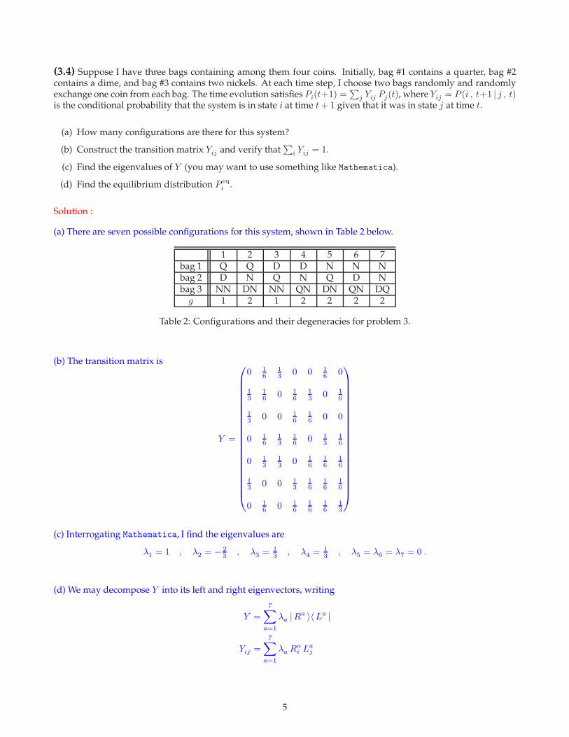
(3.4) Suppose I have three bags containing among them four coins. Initially, bag #1 contains a quarter, bag #2contains a dime, and bag #3 contains two nickels. At each time step, I choose two bags randomly and randomlyexchange one coin from each bag. The time evolution satisfies Pi(t+1) =

∑j Yij Pj(t), where Yij = P (i , t+1 | j , t)

is the conditional probability that the system is in state i at time t+ 1 given that it was in state j at time t.

(a) How many configurations are there for this system?

(b) Construct the transition matrix Yij and verify that∑

i Yij = 1.

(c) Find the eigenvalues of Y (you may want to use something like Mathematica).

(d) Find the equilibrium distribution P eqi .

Solution :

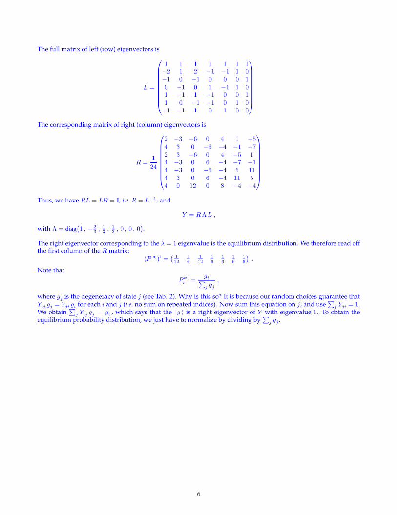
(a) There are seven possible configurations for this system, shown in Table 2 below.

1 2 3 4 5 6 7bag 1 Q Q D D N N Nbag 2 D N Q N Q D Nbag 3 NN DN NN QN DN QN DQg 1 2 1 2 2 2 2

Table 2: Configurations and their degeneracies for problem 3.

(b) The transition matrix is

Y =

0 16

13 0 0 1

6 0

13

16 0 1

613 0 1

6

13 0 0 1

616 0 0

0 16

13

16 0 1

316

0 13

13 0 1

616

16

13 0 0 1

316

16

16

0 16 0 1

616

16

13

(c) Interrogating Mathematica, I find the eigenvalues are

λ1 = 1 , λ2 = − 23 , λ3 = 1

3 , λ4 = 13 , λ5 = λ6 = λ7 = 0 .

(d) We may decompose Y into its left and right eigenvectors, writing

Y =

7∑

a=1

λa |Ra 〉〈La |

Yij =

7∑

a=1

λa Rai L

aj

5

The full matrix of left (row) eigenvectors is

L =

1 1 1 1 1 1 1−2 1 2 −1 −1 1 0−1 0 −1 0 0 0 10 −1 0 1 −1 1 01 −1 1 −1 0 0 11 0 −1 −1 0 1 0−1 −1 1 0 1 0 0

The corresponding matrix of right (column) eigenvectors is

R =1

24

2 −3 −6 0 4 1 −54 3 0 −6 −4 −1 −72 3 −6 0 4 −5 14 −3 0 6 −4 −7 −14 −3 0 −6 −4 5 114 3 0 6 −4 11 54 0 12 0 8 −4 −4

Thus, we have RL = LR = I, i.e. R = L−1, and

Y = RΛL ,

with Λ = diag(1 , − 2

3 ,13 ,

13 , 0 , 0 , 0

).

The right eigenvector corresponding to the λ = 1 eigenvalue is the equilibrium distribution. We therefore read offthe first column of the R matrix:

(P eq)t =(

112

16

112

16

16

16

16

).

Note that

P eqi =

gi∑j gj

,

where gj is the degeneracy of state j (see Tab. 2). Why is this so? It is because our random choices guarantee thatYij gj = Yji gi for each i and j (i.e. no sum on repeated indices). Now sum this equation on j, and use

∑j Yji = 1.

We obtain∑

j Yij gj = gi , which says that the | g 〉 is a right eigenvector of Y with eigenvalue 1. To obtain theequilibrium probability distribution, we just have to normalize by dividing by

∑j gj .

6

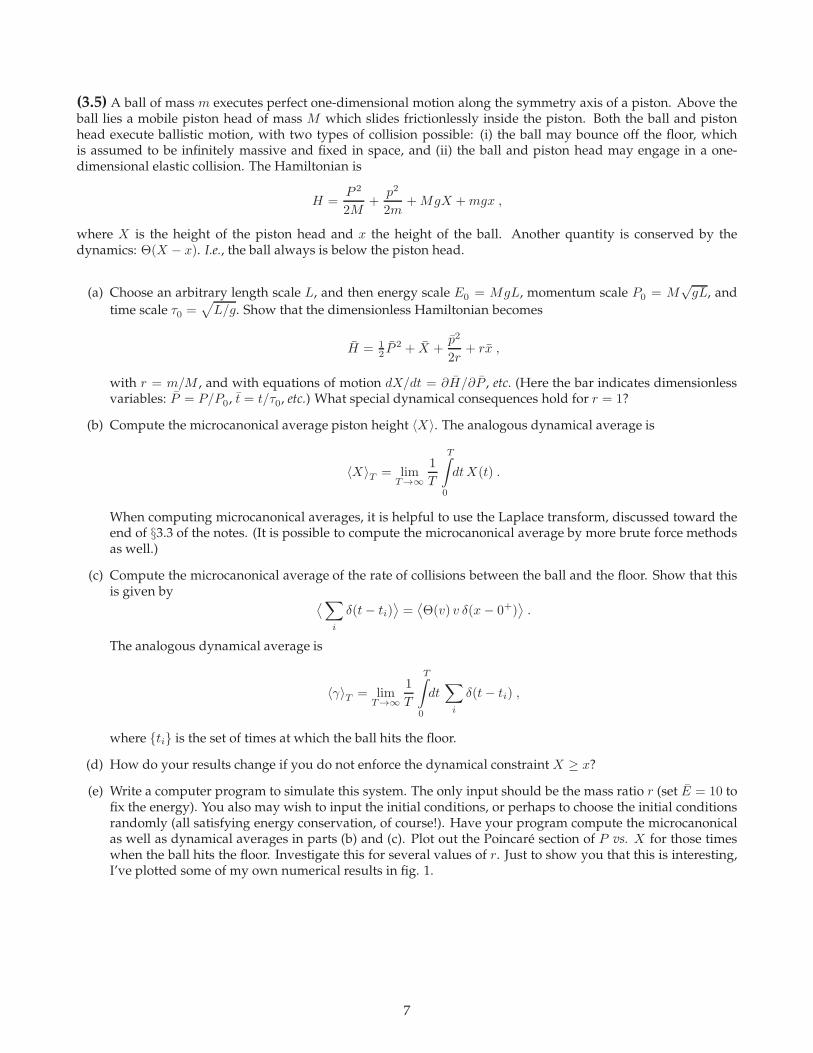
(3.5) A ball of mass m executes perfect one-dimensional motion along the symmetry axis of a piston. Above theball lies a mobile piston head of mass M which slides frictionlessly inside the piston. Both the ball and pistonhead execute ballistic motion, with two types of collision possible: (i) the ball may bounce off the floor, whichis assumed to be infinitely massive and fixed in space, and (ii) the ball and piston head may engage in a one-dimensional elastic collision. The Hamiltonian is

H =P 2

2M+

p2

2m+MgX +mgx ,

where X is the height of the piston head and x the height of the ball. Another quantity is conserved by thedynamics: Θ(X − x). I.e., the ball always is below the piston head.

(a) Choose an arbitrary length scale L, and then energy scale E0 = MgL, momentum scale P0 = M√gL, and

time scale τ0 =√L/g. Show that the dimensionless Hamiltonian becomes

H = 12 P

2 + X +p2

2r+ rx ,

with r = m/M , and with equations of motion dX/dt = ∂H/∂P , etc. (Here the bar indicates dimensionlessvariables: P = P/P0, t = t/τ0, etc.) What special dynamical consequences hold for r = 1?

(b) Compute the microcanonical average piston height 〈X〉. The analogous dynamical average is

〈X〉T = limT→∞

1

T

T∫

0

dtX(t) .

When computing microcanonical averages, it is helpful to use the Laplace transform, discussed toward theend of §3.3 of the notes. (It is possible to compute the microcanonical average by more brute force methodsas well.)

(c) Compute the microcanonical average of the rate of collisions between the ball and the floor. Show that thisis given by ⟨∑

i

δ(t− ti)⟩=

⟨Θ(v) v δ(x− 0+)

⟩.

The analogous dynamical average is

〈γ〉T = limT→∞

1

T

T∫

0

dt∑

i

δ(t− ti) ,

where {ti} is the set of times at which the ball hits the floor.

(d) How do your results change if you do not enforce the dynamical constraint X ≥ x?

(e) Write a computer program to simulate this system. The only input should be the mass ratio r (set E = 10 tofix the energy). You also may wish to input the initial conditions, or perhaps to choose the initial conditionsrandomly (all satisfying energy conservation, of course!). Have your program compute the microcanonicalas well as dynamical averages in parts (b) and (c). Plot out the Poincare section of P vs. X for those timeswhen the ball hits the floor. Investigate this for several values of r. Just to show you that this is interesting,I’ve plotted some of my own numerical results in fig. 1.

7

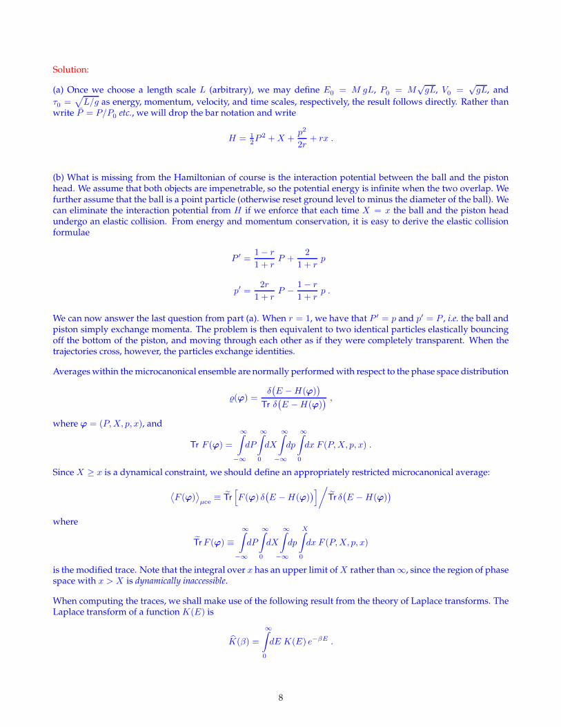
Solution:

(a) Once we choose a length scale L (arbitrary), we may define E0 = M gL, P0 = M√gL, V0 =

√gL, and

τ0 =√L/g as energy, momentum, velocity, and time scales, respectively, the result follows directly. Rather than

write P = P/P0 etc., we will drop the bar notation and write

H = 12P

2 +X +p2

2r+ rx .

(b) What is missing from the Hamiltonian of course is the interaction potential between the ball and the pistonhead. We assume that both objects are impenetrable, so the potential energy is infinite when the two overlap. Wefurther assume that the ball is a point particle (otherwise reset ground level to minus the diameter of the ball). Wecan eliminate the interaction potential from H if we enforce that each time X = x the ball and the piston headundergo an elastic collision. From energy and momentum conservation, it is easy to derive the elastic collisionformulae

P ′ =1− r

1 + rP +

2

1 + rp

p′ =2r

1 + rP − 1− r

1 + rp .

We can now answer the last question from part (a). When r = 1, we have that P ′ = p and p′ = P , i.e. the ball andpiston simply exchange momenta. The problem is then equivalent to two identical particles elastically bouncingoff the bottom of the piston, and moving through each other as if they were completely transparent. When thetrajectories cross, however, the particles exchange identities.

Averages within the microcanonical ensemble are normally performed with respect to the phase space distribution

(ϕ) =δ(E −H(ϕ)

)

Tr δ(E −H(ϕ)

) ,

where ϕ = (P,X, p, x), and

Tr F (ϕ) =

∞∫

−∞

dP

∞∫

0

dX

∞∫

−∞

dp

∞∫

0

dx F (P,X, p, x) .

Since X ≥ x is a dynamical constraint, we should define an appropriately restricted microcanonical average:

⟨F (ϕ)

⟩µce

≡ Tr[F (ϕ) δ

(E −H(ϕ)

)]/Tr δ

(E −H(ϕ)

)

where

TrF (ϕ) ≡∞∫

−∞

dP

∞∫

0

dX

∞∫

−∞

dp

X∫

0

dx F (P,X, p, x)

is the modified trace. Note that the integral over x has an upper limit ofX rather than ∞, since the region of phasespace with x > X is dynamically inaccessible.

When computing the traces, we shall make use of the following result from the theory of Laplace transforms. TheLaplace transform of a function K(E) is

K(β) =

∞∫

0

dE K(E) e−βE .

8

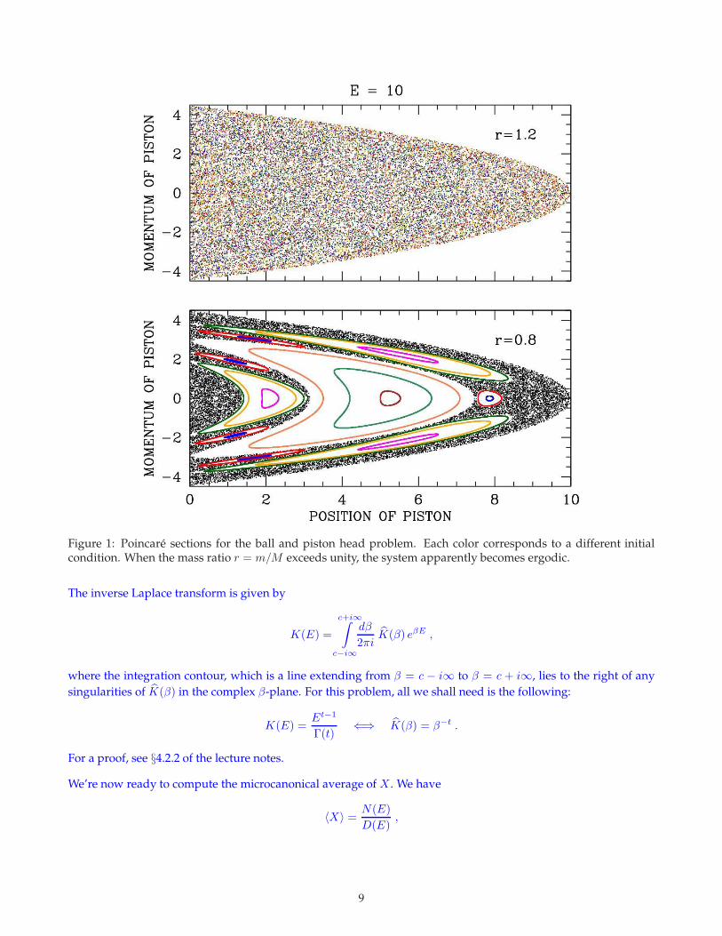
Figure 1: Poincare sections for the ball and piston head problem. Each color corresponds to a different initialcondition. When the mass ratio r = m/M exceeds unity, the system apparently becomes ergodic.

The inverse Laplace transform is given by

K(E) =

c+i∞∫

c−i∞

dβ

2πiK(β) eβE ,

where the integration contour, which is a line extending from β = c − i∞ to β = c + i∞, lies to the right of any

singularities of K(β) in the complex β-plane. For this problem, all we shall need is the following:

K(E) =Et−1

Γ(t)⇐⇒ K(β) = β−t .

For a proof, see §4.2.2 of the lecture notes.

We’re now ready to compute the microcanonical average of X . We have

〈X〉 = N(E)

D(E),

9

where

N(E) = Tr[X δ(E −H)

]

D(E) = Tr δ(E −H) .

Let’s first compute D(E). To do this, we compute the Laplace transform D(β):

D(β) = Tr e−βH

=

∞∫

−∞

dP e−βP 2/2

∞∫

−∞

dp e−βp2/2r

∞∫

0

dX e−βX

X∫

0

dx e−βrx

=2π

√r

β

∞∫

0

dX e−βX

(1− e−βrX

βr

)=

√r

1 + r· 2πβ3

.

Similarly for N(β) we have

N(β) = TrX e−βH

=

∞∫

−∞

dP e−βP 2/2

∞∫

−∞

dp e−βp2/2r

∞∫

0

dX X e−βX

X∫

0

dx e−βrx

=2π

√r

β

∞∫

0

dX X e−βX

(1− e−βrX

βr

)=

(2 + r) r3/2

(1 + r)2· 2πβ4

.

Taking the inverse Laplace transform, we then have

D(E) =

√r

1 + r· πE2 , N(E) =

(2 + r)√r

(1 + r)2· 13πE

3 .

We then have

〈X〉 = N(E)

D(E)=

(2 + r

1 + r

)· 13E .

The ‘brute force’ evaluation of the integrals isn’t so bad either. We have

D(E) =

∞∫

−∞

dP

∞∫

0

dX

∞∫

−∞

dp

X∫

0

dx δ(12P

2 + 12rp

2 +X + rx− E).

To evaluate, define P =√2ux and p =

√2r uy . Then we have dP dp = 2

√r dux duy and 1

2P2 + 1

2r p2 = u2x + u2y.

Now convert to 2D polar coordinates with w ≡ u2x + u2y . Thus,

D(E) = 2π√r

∞∫

0

dw

∞∫

0

dX

X∫

0

dx δ(w +X + rx − E

)

=2π√r

∞∫

0

dw

∞∫

0

dX

X∫

0

dx Θ(E − w −X)Θ(X + rX − E + w)

=2π√r

E∫

0

dw

E−w∫

E−w

1+r

dX =2π

√r

1 + r

E∫

0

dq q =

√r

1 + r· πE2 ,

10

with q = E − w. Similarly,

N(E) = 2π√r

∞∫

0

dw

∞∫

0

dX X

X∫

0

dx δ(w +X + rx − E

)

=2π√r

∞∫

0

dw

∞∫

0

dX X

X∫

0

dx Θ(E − w −X)Θ(X + rX − E + w)

=2π√r

E∫

0

dw

E−w∫

E−w

1+r

dX X =2π√r

E∫

0

dq

(1− 1

(1 + r)2

)· 12q

2 =

(2 + r

1 + r

)·

√r

1 + r· 13πE

3 .

(c) Using the general result

δ(F (x) −A

)=

∑

i

δ(x − xi)∣∣F ′(xi)∣∣ ,

where F (xi) = A, we recover the desired expression. We should be careful not to double count, so to avoid thisdifficulty we can evaluate δ(t− t+i ), where t+i = ti + 0+ is infinitesimally later than ti. The point here is that whent = t+i we have p = r v > 0 (i.e. just after hitting the bottom). Similarly, at times t = t−i we have p < 0 (i.e. just priorto hitting the bottom). Note v = p/r. Again we write γ(E) = N(E)/D(E), this time with

N(E) = Tr[Θ(p) r−1p δ(x− 0+) δ(E −H)

].

The Laplace transform is

N(β) =

∞∫

−∞

dP e−βP 2/2

∞∫

0

dp r−1 p e−βp2/2r

∞∫

0

dX e−βX

=

√2π

β· 1β· 1β

=√2π β−5/2 .

Thus,N(E) = 4

√2

3 E3/2

and

〈γ〉 = N(E)

D(E)= 4

√2

3π

(1 + r√r

)E−1/2 .

(d) When the constraint X ≥ x is removed, we integrate over all phase space. We then have

D(β) = Tr e−βH

=

∞∫

−∞

dP e−βP 2/2

∞∫

−∞

dp e−βp2/2r

∞∫

0

dX e−βX

∞∫

0

dx e−βrx =2π

√r

β3.

For part (b) we would then have

N(β) = Tr X e−βH

=

∞∫

−∞

dP e−βP 2/2

∞∫

−∞

dp e−βp2/2r

∞∫

0

dX X e−βX

∞∫

0

dx e−βrx =2π

√r

β4.

11

The respective inverse Laplace transforms areD(E) = π√rE2 andN(E) = 1

3π√rE3. The microcanonical average

of X would then be〈X〉 = 1

3E .

Using the restricted phase space, we obtained a value which is greater than this by a factor of (2+ r)/(1+ r). Thatthe restricted average gives a larger value makes good sense, since X is not allowed to descend below x in thatcase. For part (c), we would obtain the same result for N(E) since x = 0 in the average. We would then obtain

〈γ〉 = 4√2

3π r−1/2 E−1/2 .

The restricted microcanonical average yields a rate which is larger by a factor 1 + r. Again, it makes good sensethat the restricted average should yield a higher rate, since the ball is not allowed to attain a height greater thanthe instantaneous value of X .

(e) It is straightforward to simulate the dynamics. So long as 0 < x(t) < X(t), we have

X = P , P = −1 , x =p

r, p = −r .

Starting at an arbitrary time t0, these equations are integrated to yield

X(t) = X(t0) + P (t0) (t− t0)− 12 (t− t0)

2

P (t) = P (t0)− (t− t0)

x(t) = x(t0) +p(t0)

r(t− t0)− 1

2 (t− t0)2

p(t) = p(t0)− r(t− t0) .

We must stop the evolution when one of two things happens. The first possibility is a bounce at t = tb, meaningx(tb) = 0. The momentum p(t) changes discontinuously at the bounce, with p(t+b ) = −p(t−b ), and where p(t−b ) < 0necessarily. The second possibility is a collision at t = tc, meaning X(tc) = x(tc). Integrating across the collision,we must conserve both energy and momentum. This means

P (t+c ) =1− r

1 + rP (t−c ) +

2

1 + rp(t−c )

p(t+c ) =2r

1 + rP (t−c )−

1− r

1 + rp(t−c ) .

r X(0) 〈X(t)〉 〈X〉µce 〈γ(t)〉 〈γ〉µce r X(0) 〈X(t)〉 〈X〉µce 〈γ(t)〉 〈γ〉µce0.3 0.1 6.1743 5.8974 0.5283 0.4505 1.2 0.1 4.8509 4.8545 0.3816 0.38120.3 1.0 5.7303 5.8974 0.4170 0.4505 1.2 1.0 4.8479 4.8545 0.3811 0.38120.3 3.0 5.7876 5.8974 0.4217 0.4505 1.2 3.0 4.8493 4.8545 0.3813 0.38120.3 5.0 5.8231 5.8974 0.4228 0.4505 1.2 5.0 4.8482 4.8545 0.3813 0.38120.3 7.0 5.8227 5.8974 0.4228 0.4505 1.2 7.0 4.8472 4.8545 0.3808 0.38120.3 9.0 5.8016 5.8974 0.4234 0.4505 1.2 9.0 4.8466 4.8545 0.3808 0.38120.3 9.9 6.1539 5.8974 0.5249 0.4505 1.2 9.9 4.8444 4.8545 0.3807 0.3812

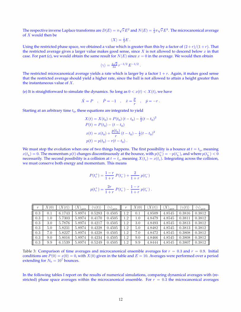
Table 3: Comparison of time averages and microcanonical ensemble averages for r = 0.3 and r = 0.9. Initialconditions are P (0) = x(0) = 0, with X(0) given in the table and E = 10. Averages were performed over a periodextending for Nb = 107 bounces.

In the following tables I report on the results of numerical simulations, comparing dynamical averages with (re-stricted) phase space averages within the microcanonical ensemble. For r = 0.3 the microcanonical averages

12

poorly approximate the dynamical averages, and the dynamical averages are dependent on the initial conditions,indicating that the system is not ergodic. For r = 1.2, the agreement between dynamical and microcanonicalaverages generally improves with averaging time. Indeed, it has been shown by N. I. Chernov, Physica D 53, 233(1991), building on the work of M. P. Wojtkowski, Comm. Math. Phys. 126, 507 (1990) that this system is ergodicfor r > 1. Wojtkowski also showed that this system is equivalent to the wedge billiard, in which a single pointparticle of mass m bounces inside a two-dimensional wedge-shaped region

{(x, y)

∣∣ x ≥ 0 , y ≥ x ctnφ}

for some

fixed angle φ = tan−1√

mM . To see this, pass to relative (X ) and center-of-mass (Y) coordinates,

X = X − x Px =mP −Mp

M +m

Y =MX +mx

M +mPy = P + p .

Then

H =(M +m)P2

x

2Mm+

P2y

2(M +m)+ (M +m) gY .

There are two constraints. One requires X ≥ x, i.e. X ≥ 0. The second requires x > 0, i.e.

x = Y − M

M +mX ≥ 0 .

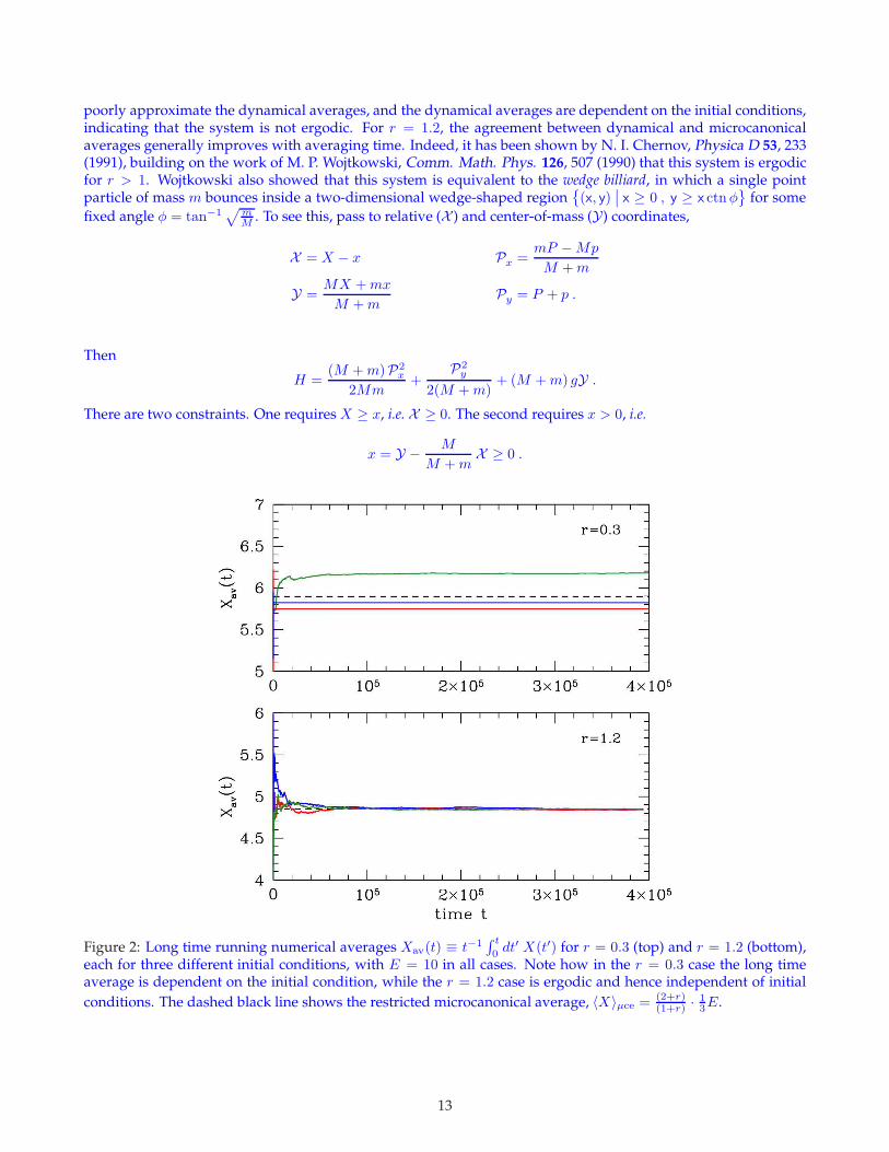
Figure 2: Long time running numerical averages Xav(t) ≡ t−1∫ t

0dt′ X(t′) for r = 0.3 (top) and r = 1.2 (bottom),

each for three different initial conditions, with E = 10 in all cases. Note how in the r = 0.3 case the long timeaverage is dependent on the initial condition, while the r = 1.2 case is ergodic and hence independent of initial

conditions. The dashed black line shows the restricted microcanonical average, 〈X〉µce = (2+r)(1+r) · 1

3E.

13

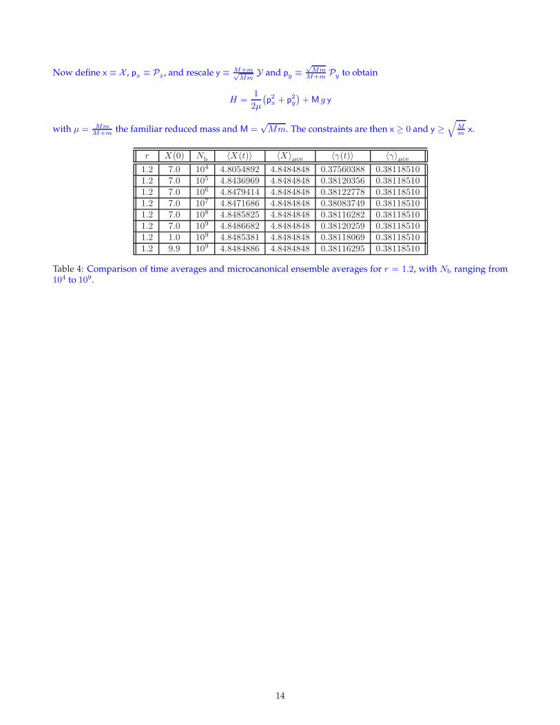
Now define x ≡ X , px ≡ Px, and rescale y ≡ M+m√Mm

Y and py ≡√Mm

M+m Py to obtain

H =1

2µ

(p2x + p2y

)+M g y

with µ = MmM+m the familiar reduced mass and M =

√Mm. The constraints are then x ≥ 0 and y ≥

√Mm x.

r X(0) Nb 〈X(t)〉 〈X〉µce 〈γ(t)〉 〈γ〉µce1.2 7.0 104 4.8054892 4.8484848 0.37560388 0.381185101.2 7.0 105 4.8436969 4.8484848 0.38120356 0.381185101.2 7.0 106 4.8479414 4.8484848 0.38122778 0.381185101.2 7.0 107 4.8471686 4.8484848 0.38083749 0.381185101.2 7.0 108 4.8485825 4.8484848 0.38116282 0.381185101.2 7.0 109 4.8486682 4.8484848 0.38120259 0.381185101.2 1.0 109 4.8485381 4.8484848 0.38118069 0.381185101.2 9.9 109 4.8484886 4.8484848 0.38116295 0.38118510

Table 4: Comparison of time averages and microcanonical ensemble averages for r = 1.2, with Nb ranging from104 to 109.

14

(3.6) Consider a toroidal phase space (x, p) ∈ T2. You can describe the torus as a square [0, 1]× [0, 1] with opposite

sides identified. Design your own modified Arnold cat map acting on this phase space, i.e. a 2 × 2 matrix withinteger coefficients and determinant 1.

(a) Start with an initial distribution localized around the center – say a disc centered at (12 ,12 ). Show how these

initial conditions evolve under your map. Can you tell whether your dynamics are mixing?

(b) Now take a pixelated image. For reasons discussed in the lecture notes, this image should exhibit Poincarerecurrence. Can you see this happening?

Solution :

(a) Any map

(x′

p′

)=

M︷ ︸︸ ︷(a bc d

) (xp

),

will due, provided det M = ad − bc = 1. Arnold’s cat map has M =

(1 11 2

). Consider the generalized cat map

with M =

(1 1p p+ 1

). Starting from an initial square distribution, we iterate the map up to three times and show

the results in Fig. 3. The numerical results are consistent with a mixing flow. (With just a few further interations,almost the entire torus is covered.)

(c) A pixelated image exhibits Poincare recurrence, as we see in Fig. 4.

Figure 3: Zeroth, first, second, and third iterates of the generalized cat map with p = 2, acting on an initial squaredistribution (clockwise from upper left).

15

(3.7) Consider a modified version of the Kac ring model where each spin exists in one of three states: A, B, or C.The flippers rotate the internal states cyclically: A→B→C→A.

(a) What is the Poincare recurrence time for this system? Hint: the answer depends on whether or not the totalnumber of flippers is a multiple of 3.

(b) Simulate the system numerically. Choose a ring size on the order ofN = 10, 000 and investigate a few flipperdensities: x = 0.001, x = 0.01, x = 0.1, x = 0.99. Remember that the flippers are located randomly at thestart, but do not move as the spins evolve. Starting from a configuration where all the spins are in the Astate, plot the probabilities pA(t), pB(t), and pC(t) versus the discrete time coordinate t, with t ranging from 0to the recurrence time. If you can, for each value of x, plot the three probabilities in different colors or linecharacteristics (e.g. solid, dotted, dashed) on the same graph.

(c) Let’s call at = pA(t), etc. Explain in words why the Stosszahlansatz results in the equations

at+1 = (1− x) at + x ct

bt+1 = (1− x) bt + xat

ct+1 = (1− x) ct + x bt .

This describes what is known as a Markov process, which is governed by coupled equations of the formPi(t + 1) =

∑j Qij Pj(t), where Q is the transition matrix. Find the 3 × 3 transition matrix for this Markov

process.

(d) Show that the total probability is conserved by a Markov process if∑

iQij = 1 and verify this is the case forthe equations in (c).

(e) One can then eliminate ct = 1− at − bt and write these as two coupled equations. Show that if we define

at ≡ at − 13 , bt ≡ bt − 1

3 , ct ≡ ct − 13

that we can write (at+1

bt+1

)= R

(atbt

),

and find the 2× 2 matrix R. Note that this is not a Markov process in A and B, since total probability for theA and B states is not itself conserved. Show that the eigenvalues of R form a complex conjugate pair. Findthe amplitude and phase of these eigenvalues. Show that the amplitude never exceeds unity.

(f) The fact that the eigenvalues of R are complex means that the probabilities should oscillate as they decay totheir equilibrium values p

A= p

B= p

C= 1

3 . Can you see this in your simulations?

Solution :

(a) If the number of flippers Nf is a multiple of 3, then each spin will have made an integer number of completecyclic changes A→B→C→A after one complete passage around the ring. The recurrence time is then N , where Nis the number of sites. If the number of flippers Nf is not a multiple of 3, then the recurrence time is simply 3N .

(b) See figs. 5, 6, 7.

(c) According to the Stosszahlansatz, the probability at+1 that a given spin will be in state A at time (t + 1) isthe probability at it was in A at time t times the probability (1 − x) that it did not encounter a flipper, plus theprobability ct it was in state C at time t times the probability x that it did encounter a flipper. This explains thefirst equation. The others follow by cyclic permutation. The transition matrix is

Q =

1− x 0 xx 1− x 00 x 1− x

.

16

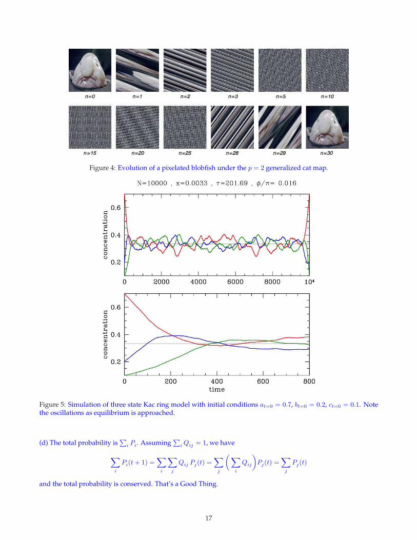
Figure 4: Evolution of a pixelated blobfish under the p = 2 generalized cat map.

Figure 5: Simulation of three state Kac ring model with initial conditions at=0 = 0.7, bt=0 = 0.2, ct=0 = 0.1. Notethe oscillations as equilibrium is approached.

(d) The total probability is∑

i Pi. Assuming∑

iQij = 1, we have

∑

i

Pi(t+ 1) =∑

i

∑

j

Qij Pj(t) =∑

j

(∑

i

Qij

)Pj(t) =

∑

j

Pj(t)

and the total probability is conserved. That’s a Good Thing.

17

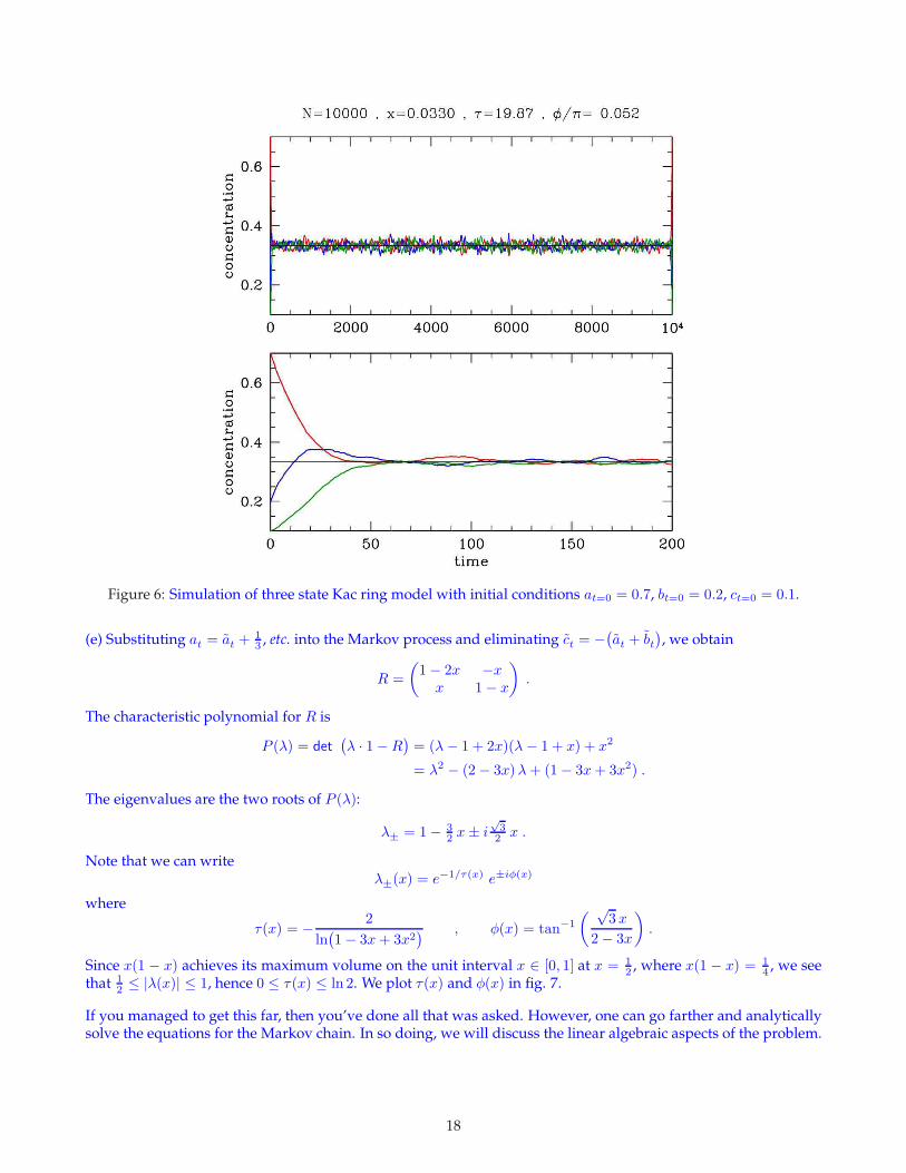
Figure 6: Simulation of three state Kac ring model with initial conditions at=0 = 0.7, bt=0 = 0.2, ct=0 = 0.1.

(e) Substituting at = at +13 , etc. into the Markov process and eliminating ct = −

(at + bt

), we obtain

R =

(1− 2x −xx 1− x

).

The characteristic polynomial for R is

P (λ) = det(λ · 1−R

)= (λ− 1 + 2x)(λ − 1 + x) + x2

= λ2 − (2 − 3x)λ+ (1− 3x+ 3x2) .

The eigenvalues are the two roots of P (λ):

λ± = 1− 32 x± i

√32 x .

Note that we can writeλ±(x) = e−1/τ(x) e±iφ(x)

where

τ(x) = − 2

ln(1− 3x+ 3x2

) , φ(x) = tan−1

( √3 x

2− 3x

).

Since x(1 − x) achieves its maximum volume on the unit interval x ∈ [0, 1] at x = 12 , where x(1 − x) = 1

4 , we seethat 1

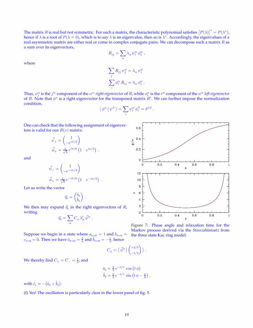
2 ≤ |λ(x)| ≤ 1, hence 0 ≤ τ(x) ≤ ln 2. We plot τ(x) and φ(x) in fig. 7.

If you managed to get this far, then you’ve done all that was asked. However, one can go farther and analyticallysolve the equations for the Markov chain. In so doing, we will discuss the linear algebraic aspects of the problem.

18

The matrixR is real but not symmetric. For such a matrix, the characteristic polynomial satisfies[P (λ)

]∗= P (λ∗),

hence if λ is a root of P (λ = 0), which is to say λ is an eigenvalue, then so is λ∗. Accordingly, the eigenvalues of areal asymmetric matrix are either real or come in complex conjugate pairs. We can decompose such a matrix R asa sum over its eigenvectors,

Rij =∑

α

λα ψαi φ

αj ,

where∑

j

Rij ψαj = λα ψ

αi

∑

i

φαi Rij = λα φαj .

Thus, ψαj is the jth component of the αth right eigenvector ofR, while φαi is the ith component of the αth left eigenvector

of R. Note that φα is a right eigenvector for the transposed matrix Rt. We can further impose the normalizationcondition, ⟨

φα∣∣ψβ

⟩=

∑

i

ψαi φ

βi = δαβ .

Figure 7: Phase angle and relaxation time for theMarkov process derived via the Stosszahlansatz fromthe three state Kac ring model.

One can check that the following assignment of eigenvec-tors is valid for our R(x) matrix:

~ψ+ =

(1

−eiπ/3)

~φ+ = 1√3eiπ/6

(1 eiπ/3

).

and

~ψ− =

(1

−e−iπ/3

)

~φ+ = 1√3e−iπ/6

(1 e−iπ/3

).

Let us write the vector

~ηt =

(atbt

).

We then may expand ~ηt in the right eigenvectors of R,writing

~ηt =∑

α

Cα λtα~ψα .

Suppose we begin in a state where at=0 = 1 and bt=0 =

ct=0 = 0. Then we have at=0 = 23 and bt=0 = − 1

3 , hence

Cα =⟨~φα

∣∣(

+2/3

−1/3

)⟩.

We thereby find C+ = C− = 13 , and

at =23 e

−t/τ cos(t φ

)

bt =23 e

−t/τ sin(t φ− π

6

),

with ct = −(at + bt

).

(f) Yes! The oscillation is particularly clear in the lower panel of fig. 5.

19

(3.8) Consider a spin singlet formed by two S = 12 particles, |Ψ 〉 = 1√

2

(|↑

A↓B〉 − |↓

A↑B〉). Find the reduced

density matrix, ρA= Tr

B|Ψ 〉〈Ψ |.

Solution :

We have|Ψ 〉〈Ψ | = 1

2 |↑A ↓B 〉〈 ↑A ↓B |+ 12 |↓A ↑B 〉〈 ↓A ↑B | − 1

2 |↑A ↓B 〉〈 ↓A ↑B | − 12 |↓A ↑B 〉〈 ↑A ↓B | .

Now take the trace over the spin degrees of freedom on site B. Only the first two terms contribute, resulting in thereduced density matrix

ρA= Tr

B|Ψ 〉〈Ψ | = 1

2 |↑A 〉〈 ↑A |+ 12 |↓A 〉〈 ↓A | .

Note that Tr ρA= 1, but whereas the full density matrix ρ = Tr

B|Ψ 〉〈Ψ | had one eigenvalue of 1, corresponding

to eigenvector |Ψ 〉, and three eigenvalues of 0, corresponding to any state orthogonal to |Ψ 〉, the reduced densitymatrix ρ

Adoes not correspond to a ‘pure state’ in that it is not a projector. It has two degenerate eigenvalues at

λ = 12 . The quantity S

A= −Tr ρ

Aln ρ

A= ln 2 is the quantum entanglement entropy for the spin singlet.

20