Topics

• spatial encoding - part 2

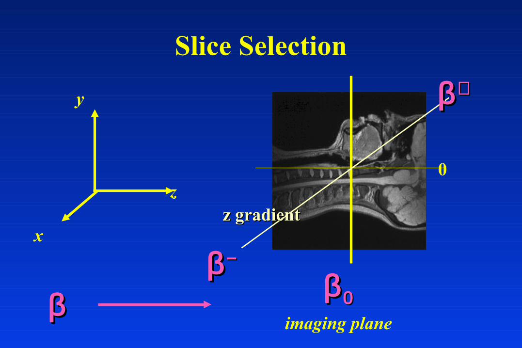
Slice Selection

ββ

z

y

x

0

imaging plane

ββ ++

ββ −−

ββ 00

z gradientz gradient

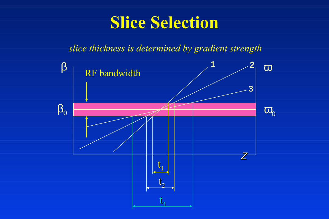
Slice Selectionslice thickness is determined by gradient strength

β

β0

ω

ω0

RF bandwidth1

3

2

ΖΖtt11

tt22

tt33

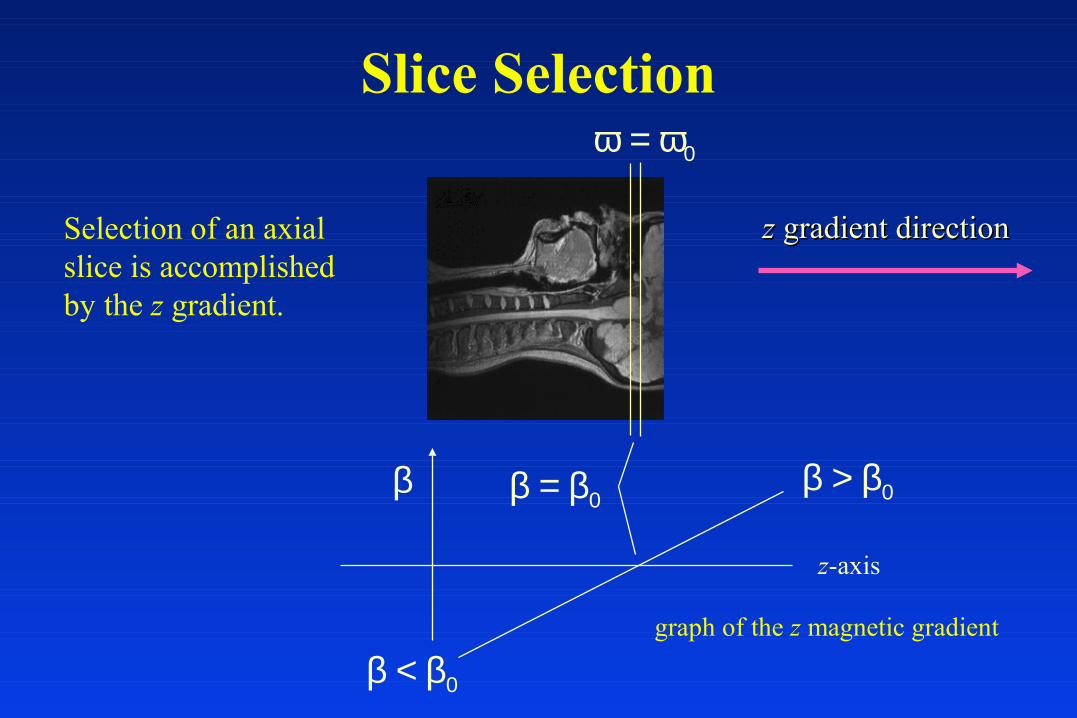
Slice Selection

Selection of an axial slice is accomplished by the z gradient.

zz gradient direction gradient direction

ω = ω0

graph of the z magnetic gradient

z-axis

β β = β0β > β0

β < β0

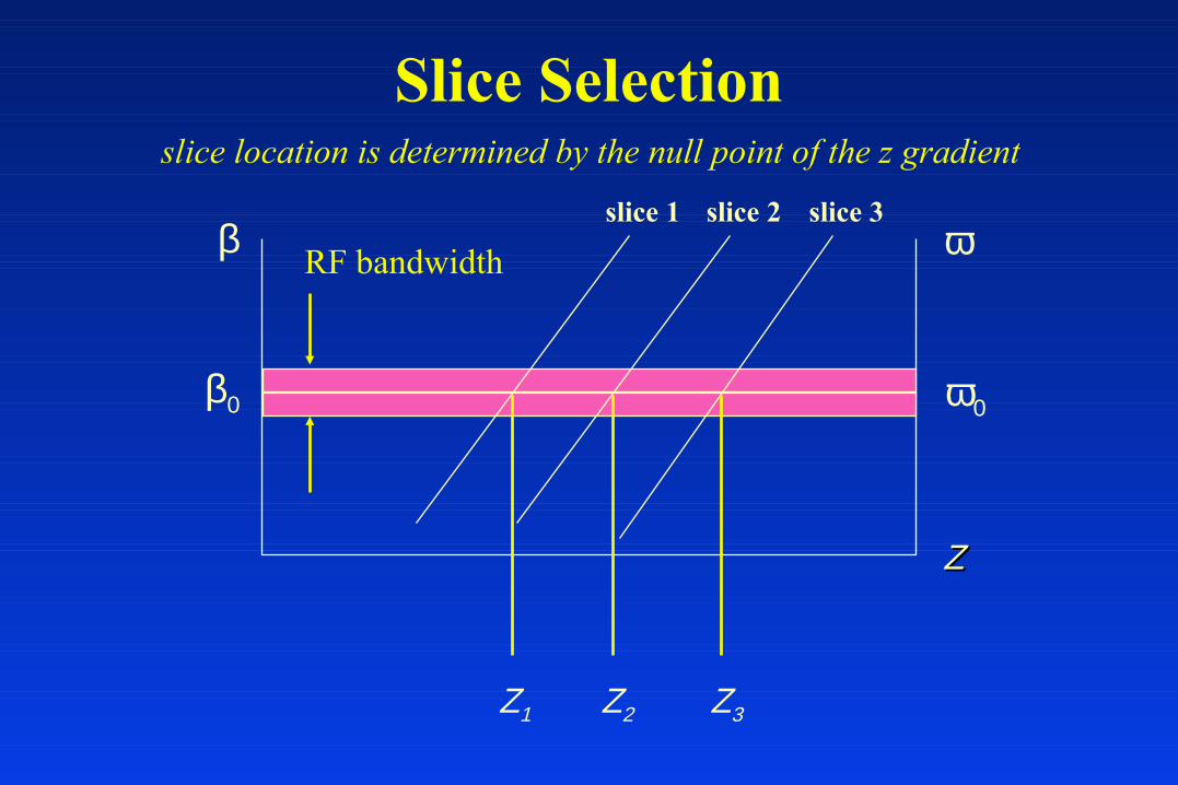
Slice Selectionslice location is determined by the null point of the z gradient

β

β0

ω

ω0

RF bandwidth

slice 1

ΖΖ

slice 2 slice 3

Ζ1 Ζ2 Ζ3

Frequency Encoding

• Within the imaging plane, a small gradient is applied left to right to allow for spatial encoding in the x direction.

• Tissues on the left will have a slightly higher resonance frequency than tissues on the right.

• The superposition of an x gradient on the patient is called frequency encoding.

• Frequency encoding enables spatial localization in the L-R direction only.

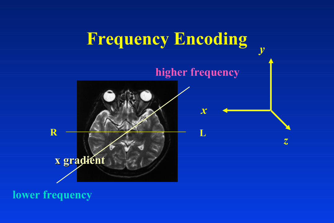
Frequency Encoding

z

y

x

x gradientx gradient

higher frequency

lower frequency

LR

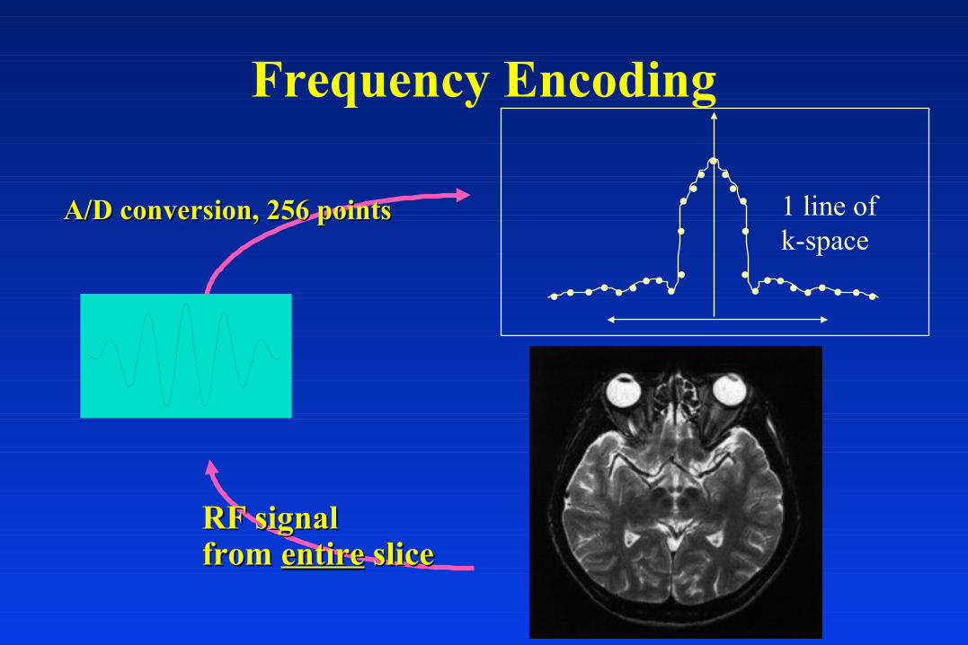
Frequency Encoding

RF signal RF signal from from entireentire slice slice

A/D conversion, 256 pointsA/D conversion, 256 points 1 line ofk-space

Phase Encoding

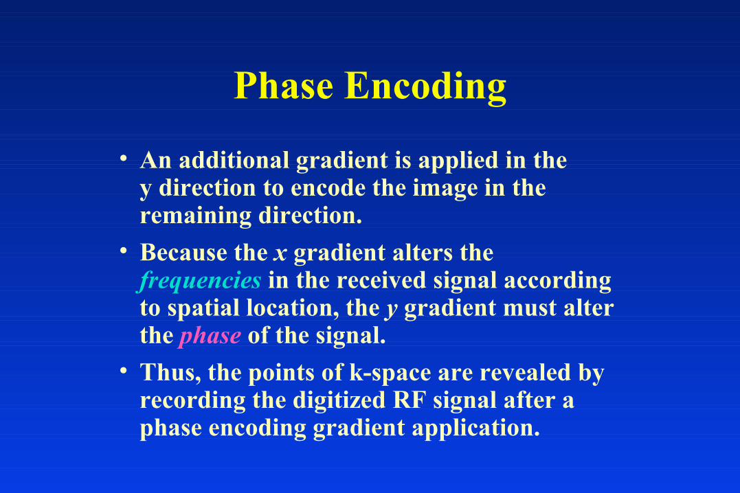
• An additional gradient is applied in the y direction to encode the image in the remaining direction.

• Because the x gradient alters the frequencies in the received signal according to spatial location, the y gradient must alter the phase of the signal.

• Thus, the points of k-space are revealed by recording the digitized RF signal after a phase encoding gradient application.

Phase Encoding

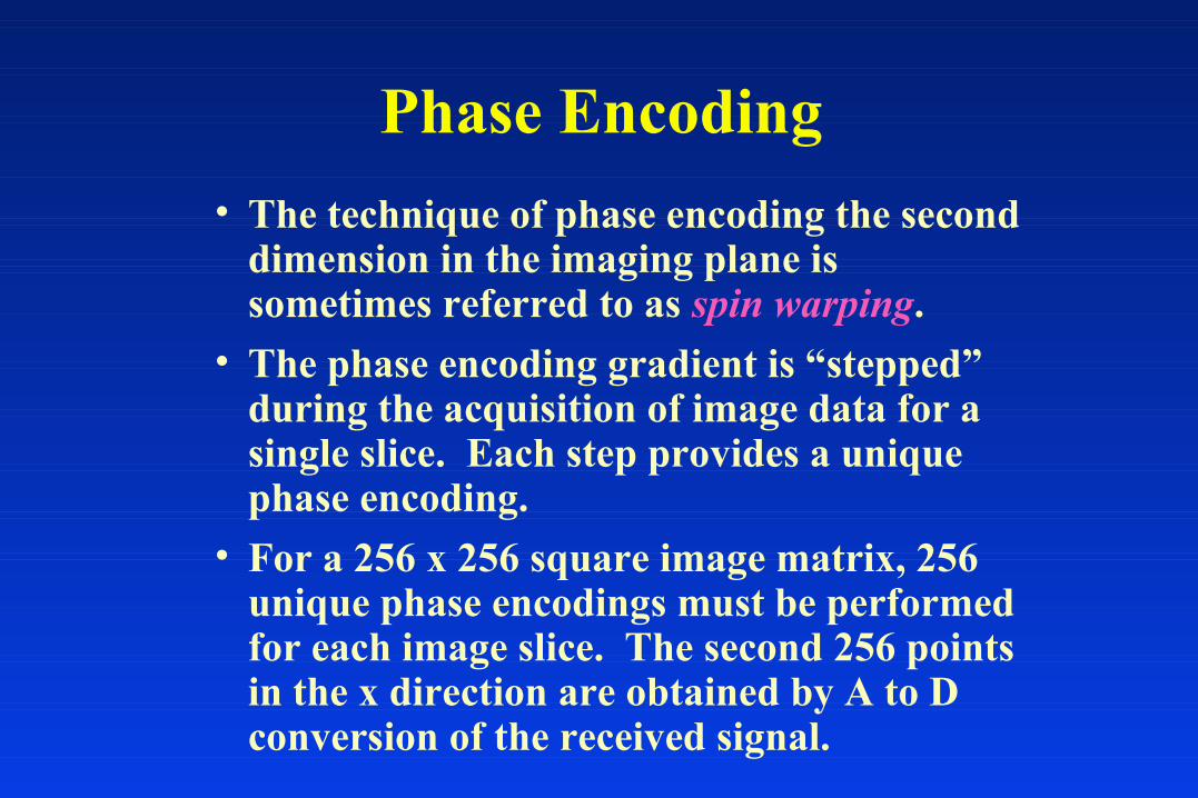
• The technique of phase encoding the second dimension in the imaging plane is sometimes referred to as spin warping.

• The phase encoding gradient is “stepped” during the acquisition of image data for a single slice. Each step provides a unique phase encoding.

• For a 256 x 256 square image matrix, 256 unique phase encodings must be performed for each image slice. The second 256 points in the x direction are obtained by A to D conversion of the received signal.

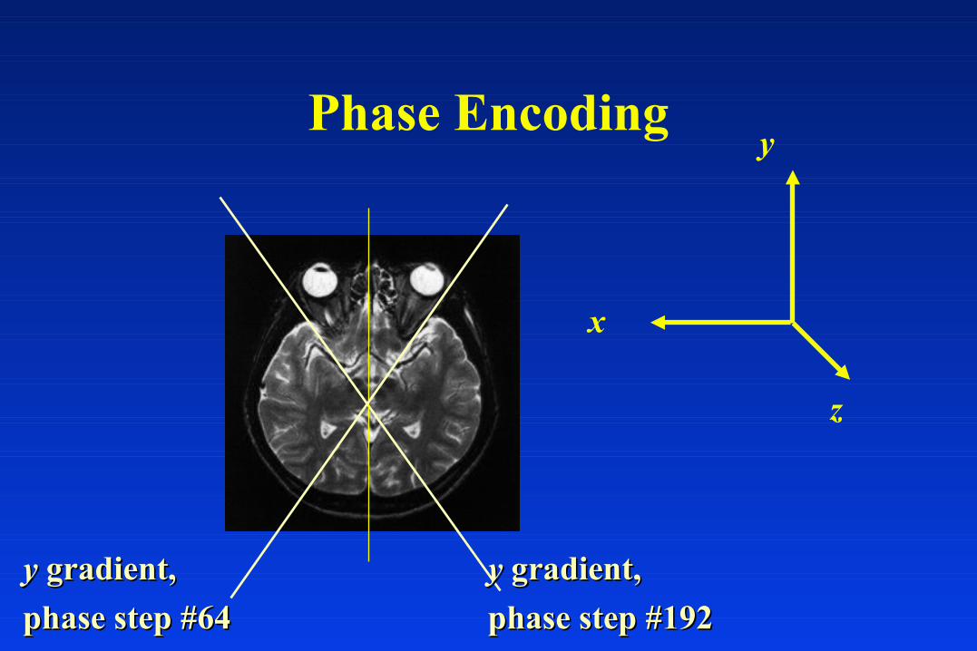
Phase Encoding

z

y

x

yy gradient, gradient,

phase step #192phase step #192

yy gradient, gradient,

phase step #64phase step #64

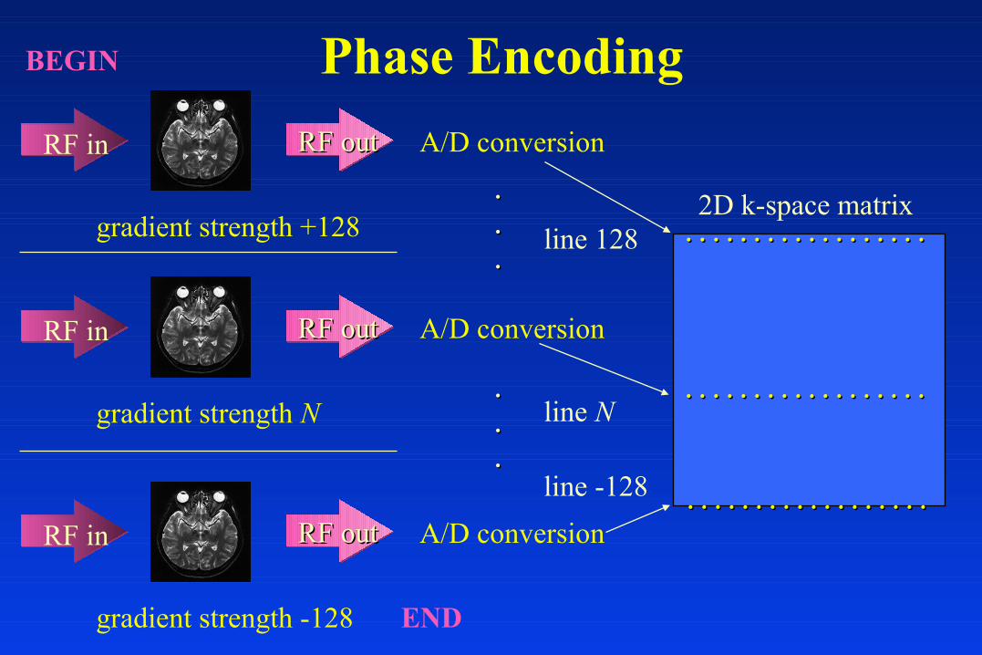
Phase Encoding

2D k-space matrixgradient strength +128

RF in RF outRF out A/D conversion

gradient strength N

RF in RF outRF out A/D conversion

gradient strength -128

RF in RF outRF out A/D conversion

END

BEGIN

line 128

line N

line -128

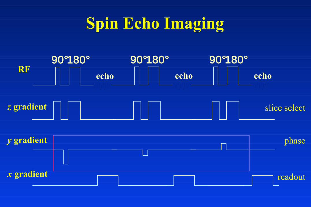
Spin Echo Imaging

RF

z gradient

echo

90°180°echo

90°180°echo

90°180°

y gradient

x gradient

slice select

phase

readout

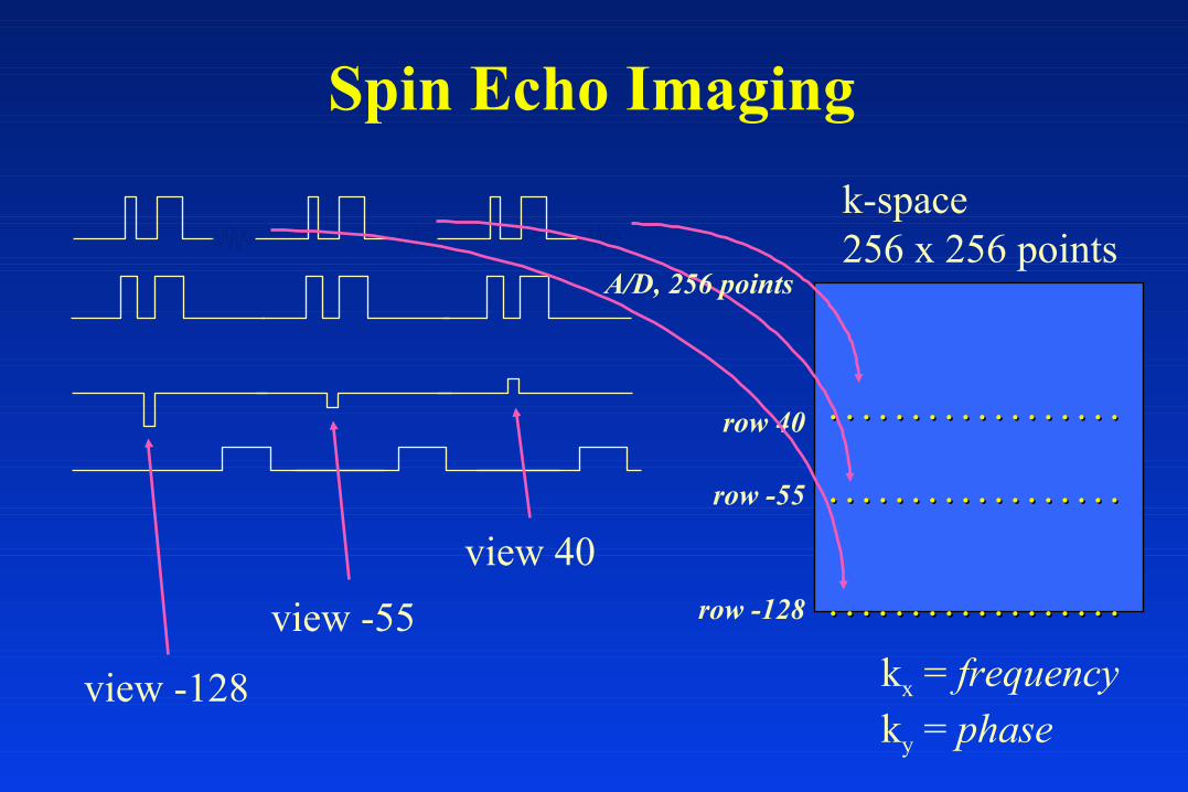
Spin Echo Imaging

view -128

view -55

view 40

k-space256 x 256 points

row 40

row -55

row -128

A/D, 256 points

kx = frequencyky = phase

• Acquisition of spatially encoded data as described allows for reconstruction of the MR image.

• The frequency and phase data are acquired and form points in a 2D array .

• Reconstruction of the image is provided by 2D inverse Fourier transform of the 2D array.

• This method of spatially encoding the MR image is called 2D FT imaging.

MR Image Reconstruction

Discrete Fourier Transform

F(kx,ky) is the 2D discrete Fourier transform of the image f(x,y)

f x yN

F k k exk yk

kkx y

jN

x jN

yNN

yx

( , ) ( , )=+

=

−

=

−

∑∑12

2 2

0

1

0

1 π π

x

y

f(x,y)

kx

ky

ℑ

k-space

F(kx,ky)

MR image

Image Resolution and Phase Encoding• Resolution is always maximum in the

frequency encoding direction because the MR signal is always digitized into 256 points.

• Resolution can vary in the phase encoding direction depending on the number of phase steps used to acquire the image.

• Because each phase encoding requires a separate 90 and 180 degree pulse, image acquisition time is proportional to the number of phase encode steps.

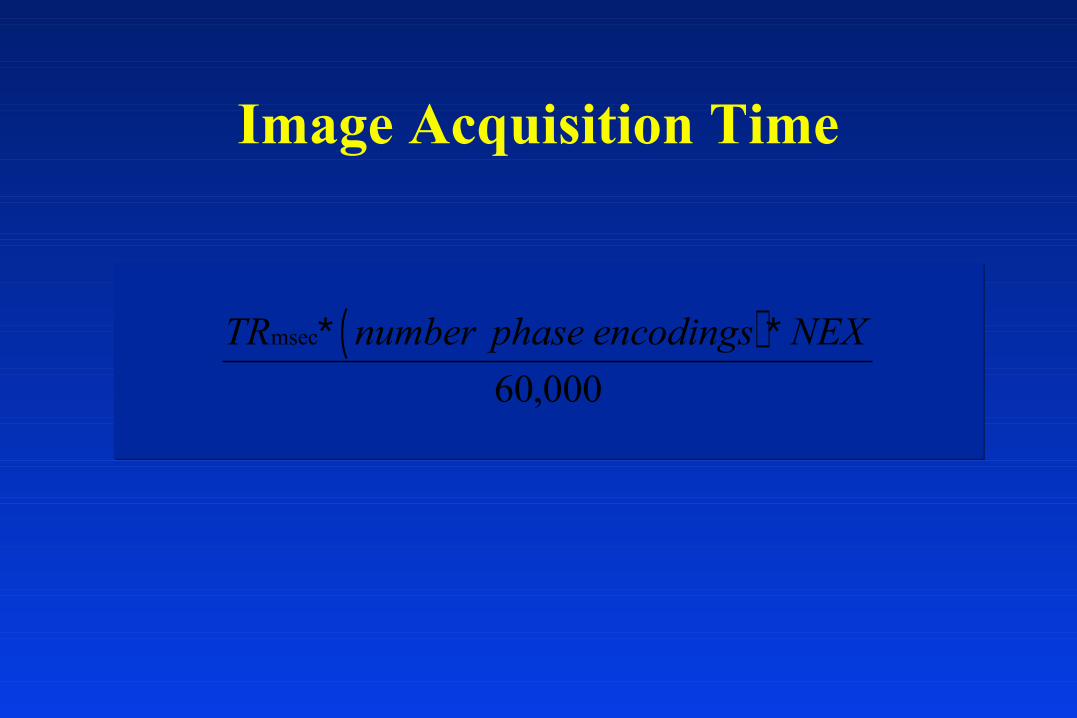
Image Acquisition Time

( )TR number phase encodings NEXmsec∗ ∗60,000

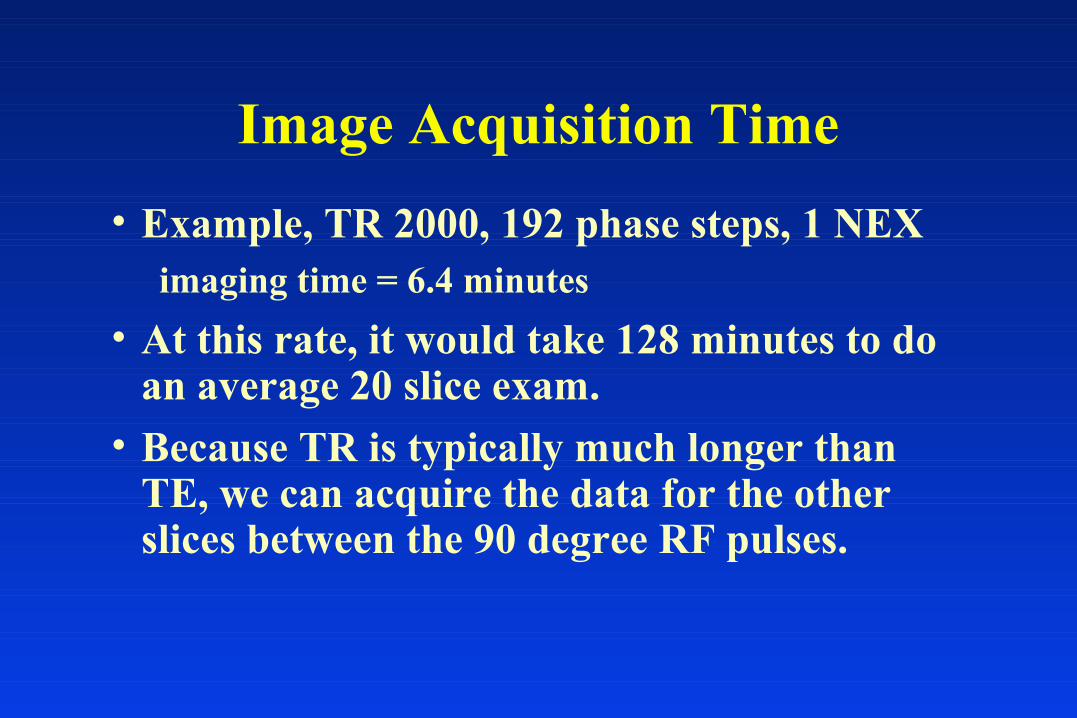
• Example, TR 2000, 192 phase steps, 1 NEXimaging time = 6.4 minutes

• At this rate, it would take 128 minutes to do an average 20 slice exam.

• Because TR is typically much longer than TE, we can acquire the data for the other slices between the 90 degree RF pulses.

Image Acquisition Time

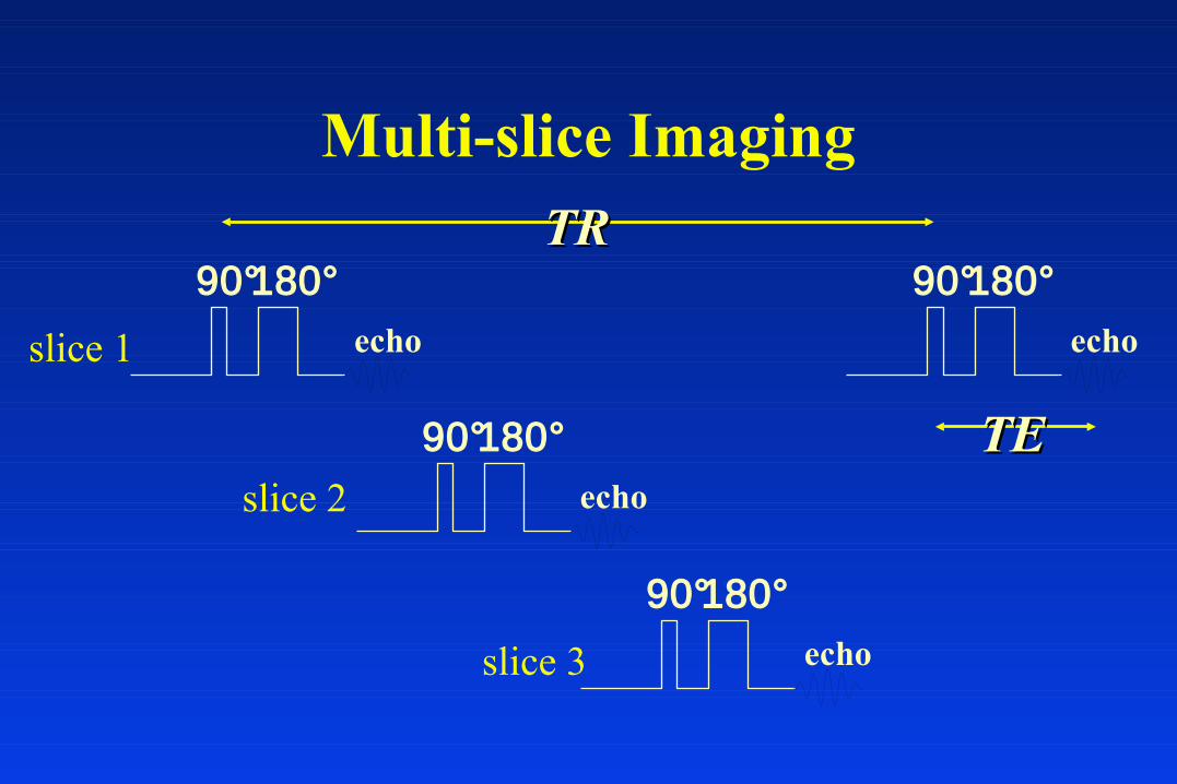
Multi-slice Imaging

echo

90°180°

echo

90°180°

echo

90°180°

echo

90°180°

slice 1

slice 2

slice 3

TRTR

TETE

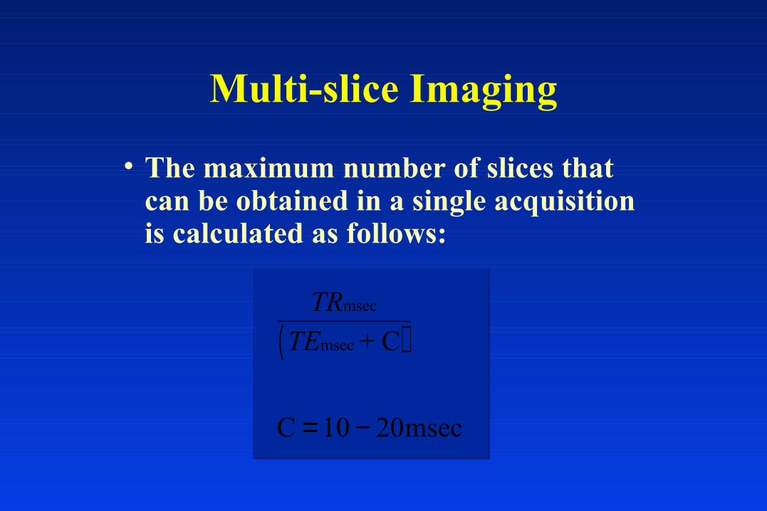
• The maximum number of slices that can be obtained in a single acquisition is calculated as follows:

Multi-slice Imaging

( )TR

TE

msec

msec + C

C msec= −10 20

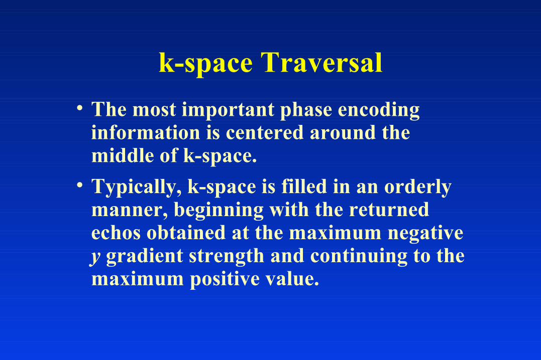
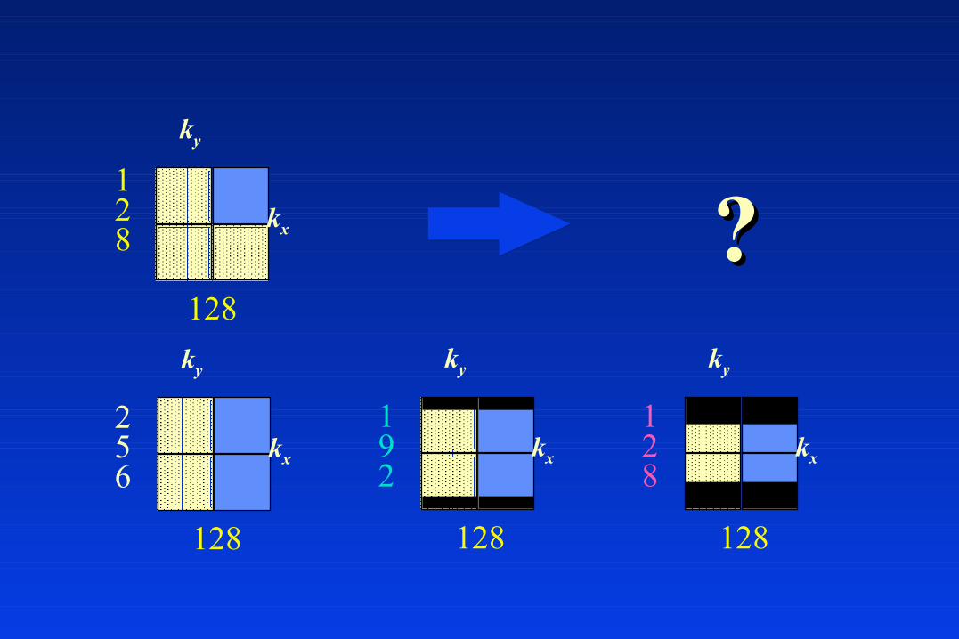
k-space Traversal

• The most important phase encoding information is centered around the middle of k-space.

• Typically, k-space is filled in an orderly manner, beginning with the returned echos obtained at the maximum negative y gradient strength and continuing to the maximum positive value.

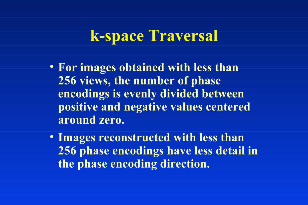
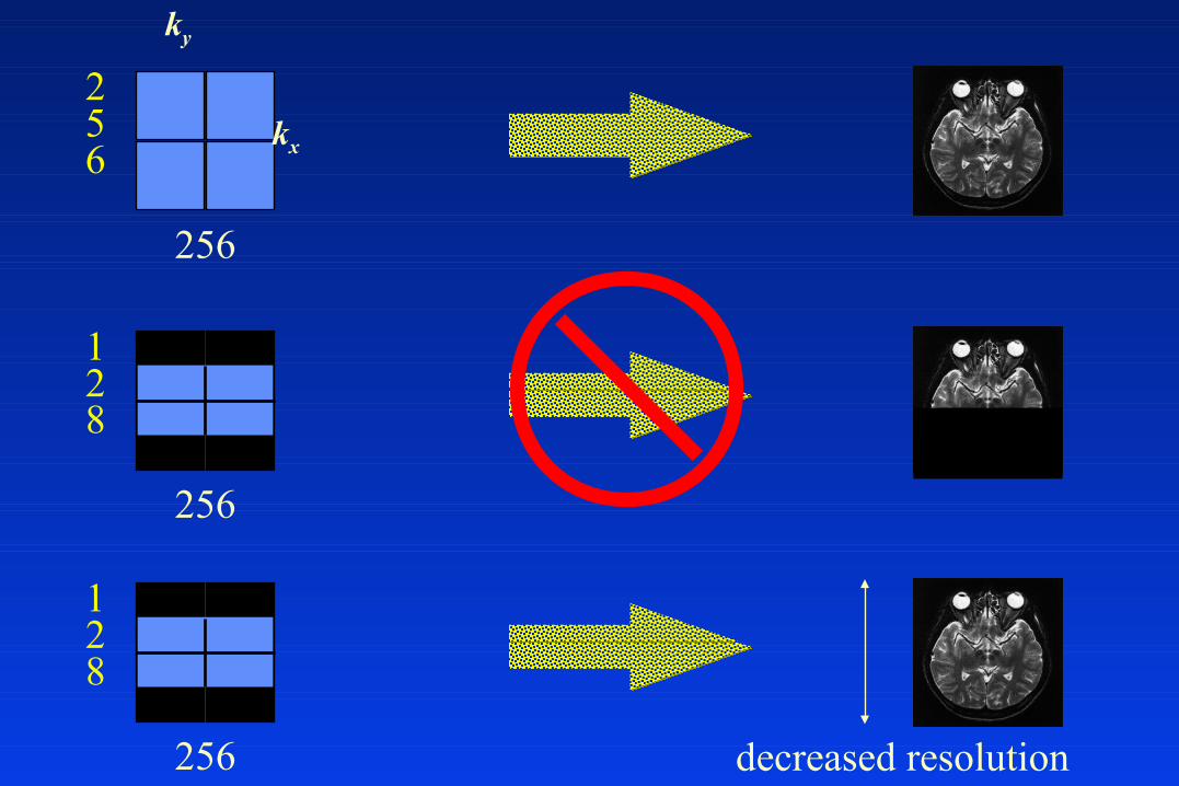
• For images obtained with less than 256 views, the number of phase encodings is evenly divided between positive and negative values centered around zero.

• Images reconstructed with less than 256 phase encodings have less detail in the phase encoding direction.

k-space Traversal

kx

ky

256

256

256

128

256

128

decreased resolution

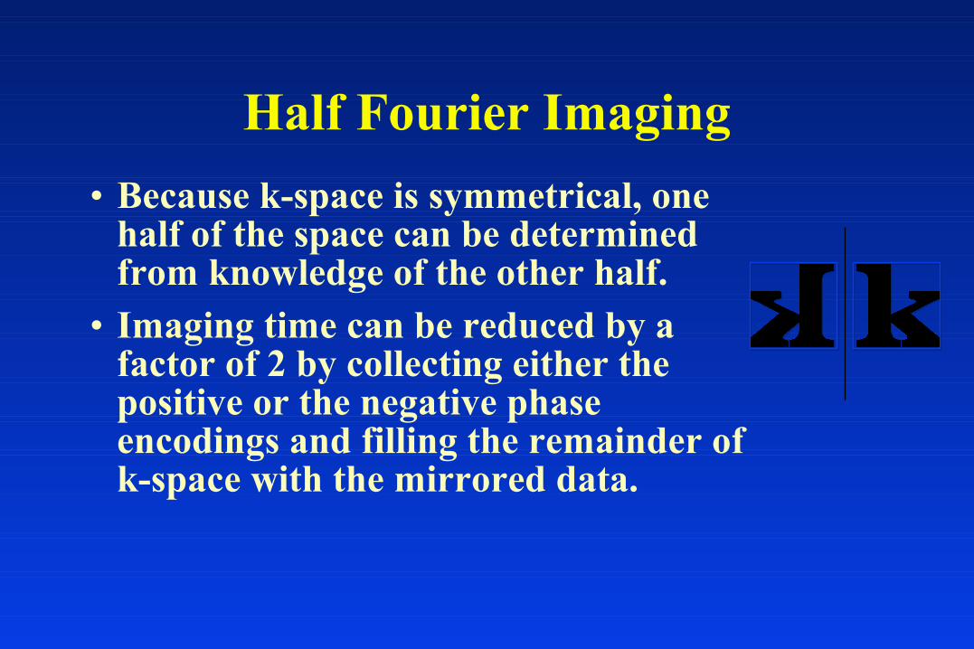
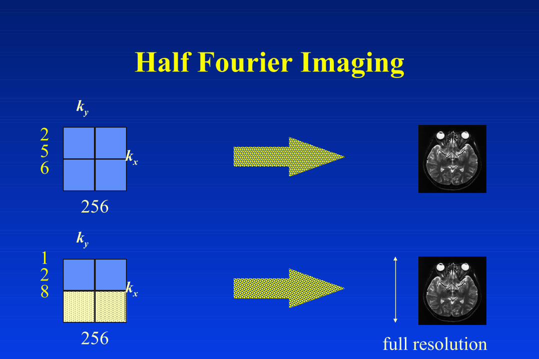
• Because k-space is symmetrical, one half of the space can be determined from knowledge of the other half.

• Imaging time can be reduced by a factor of 2 by collecting either the positive or the negative phase encodings and filling the remainder of k-space with the mirrored data.

Half Fourier Imaging

Half Fourier Imaging

kx

ky

256

256

kx

ky

256

128

full resolution

• This technique is sometimes referred to as ‘half NEX’ imaging or ‘PCS’ (phase conjugate symmetry).

• Penalty: reduced signal decreases the signal to noise ratio, typically by a factor of 0.71.

Half Fourier Imaging

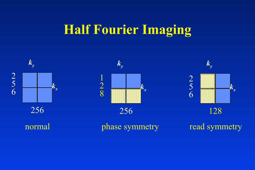
• The frequency half of k-space can also be mirrored.

• This technique is called fractional echo or ‘RCS’ (read conjugate symmetry).

• Decreased read time enables more slices per acquisition at the expense of reduced signal.

Half Fourier Imaging

Half Fourier Imaging

kx

ky

256

256

256

kx

ky

128

normal phase symmetry

kx

ky

128

256

read symmetry

kx

ky

128

128 ??

128

kx

ky

256

128

kx

ky

192

128

kx

ky

128

3D Acquisition

• 3D is an extension of the 2D technique.

advantages:

true contiguous slices

very thin slices (< 1 mm)

no partial volume effects

volume data acquisition

disadvantages:

gradient echo imaging only

(3D FSE now available)

motion sensitive

3D Acquisition

• no slice select gradient

• entire volume of tissue is excited

• second phase encoding gradient replaces the slice select gradient

• after the intial RF pulse (α), both y and z gradients are applied, followed by application of the x gradient during readout (echo)

• the z gradient is changed only after all of the y gradient phase encodes have generated an echo, then the z gradient is stepped and the y gradient phase encodes are repeated

3D Acquisition

( ) ( )TR number phase encodings number phase encodings NEXmsec∗ ° ∗ ° ∗1 2

60,000

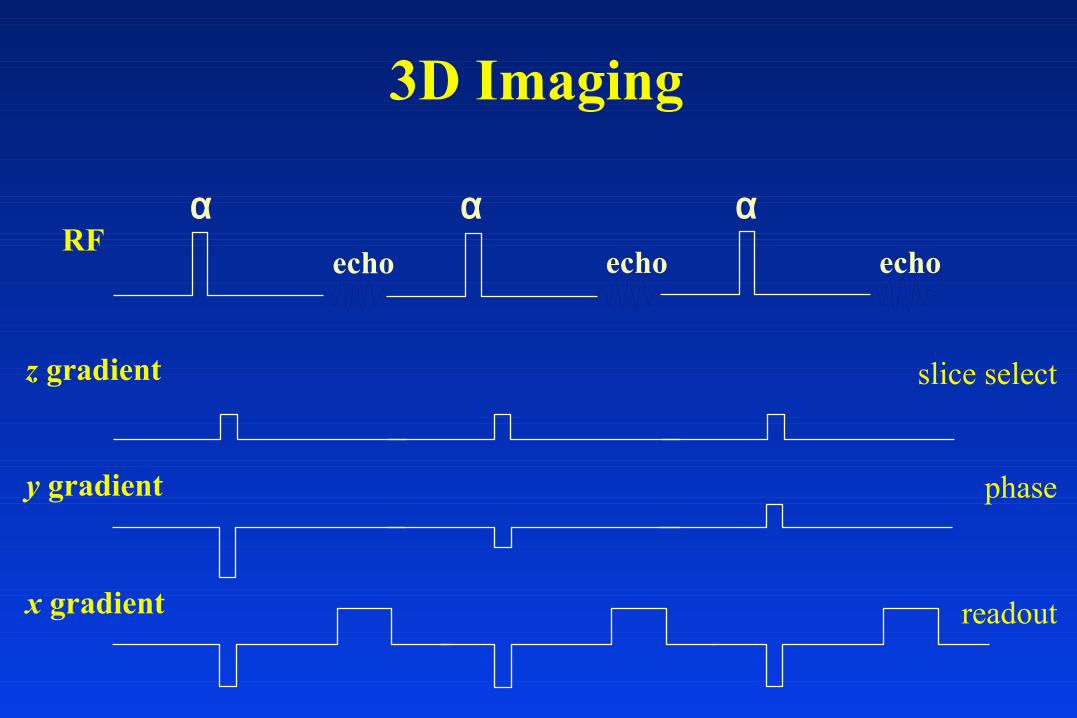
3D Imaging

RF

z gradient

echo

αecho

αecho

α

y gradient

x gradient

slice select

phase

readout

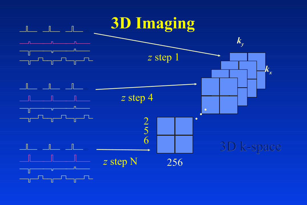
3D Imaging

kx

ky

256

256

z step 1

z step 4

z step N3D k-space3D k-space