2.5 CONTINUUM MECHANICS (FLUIDS)
43
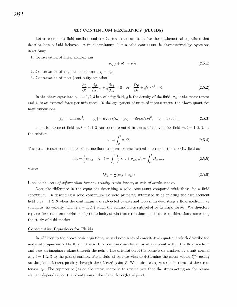
282 §2.5 CONTINUUM MECHANICS (FLUIDS) Let us consider a fluid medium and use Cartesian tensors to derive the mathematical equations that describe how a fluid behaves. A fluid continuum, like a solid continuum, is characterized by equations describing: 1. Conservation of linear momentum σ ij,j + %b i = % ˙ v i (2.5.1) 2. Conservation of angular momentum σ ij = σ ji . 3. Conservation of mass (continuity equation) ∂% ∂t + ∂% ∂x i v i + % ∂v i ∂x i =0 or D% Dt + %∇· ~ V =0. (2.5.2) In the above equations v i ,i =1, 2, 3 is a velocity field, % is the density of the fluid, σ ij is the stress tensor and b j is an external force per unit mass. In the cgs system of units of measurement, the above quantities have dimensions [˙ v j ] = cm/sec 2 , [b j ]= dynes/g, [σ ij ]= dyne/cm 2 , [%]= g/cm 3 . (2.5.3) The displacement field u i ,i =1, 2, 3 can be represented in terms of the velocity field v i ,i =1, 2, 3, by the relation u i = Z t 0 v i dt. (2.5.4) The strain tensor components of the medium can then be represented in terms of the velocity field as e ij = 1 2 (u i,j + u j,i )= Z t 0 1 2 (v i,j + v j,i ) dt = Z t 0 D ij dt, (2.5.5) where D ij = 1 2 (v i,j + v j,i ) (2.5.6) is called the rate of deformation tensor , velocity strain tensor, or rate of strain tensor. Note the difference in the equations describing a solid continuum compared with those for a fluid continuum. In describing a solid continuum we were primarily interested in calculating the displacement field u i ,i =1, 2, 3 when the continuum was subjected to external forces. In describing a fluid medium, we calculate the velocity field v i ,i =1, 2, 3 when the continuum is subjected to external forces. We therefore replace the strain tensor relations by the velocity strain tensor relations in all future considerations concerning the study of fluid motion. Constitutive Equations for Fluids In addition to the above basic equations, we will need a set of constitutive equations which describe the material properties of the fluid. Toward this purpose consider an arbitrary point within the fluid medium and pass an imaginary plane through the point. The orientation of the plane is determined by a unit normal n i , i =1, 2, 3 to the planar surface. For a fluid at rest we wish to determine the stress vector t (n) i acting on the plane element passing through the selected point P. We desire to express t (n) i in terms of the stress tensor σ ij . The superscript (n) on the stress vector is to remind you that the stress acting on the planar element depends upon the orientation of the plane through the point.
Transcript of 2.5 CONTINUUM MECHANICS (FLUIDS)
282
§2.5 CONTINUUM MECHANICS (FLUIDS)
Let us consider a fluid medium and use Cartesian tensors to derive the mathematical equations that
describe how a fluid behaves. A fluid continuum, like a solid continuum, is characterized by equations
describing:
1. Conservation of linear momentum
σij,j + %bi = %vi (2.5.1)
2. Conservation of angular momentum σij = σji.
3. Conservation of mass (continuity equation)
∂%
∂t+
∂%
∂xivi + %
∂vi
∂xi= 0 or
D%
Dt+ %∇ · ~V = 0. (2.5.2)
In the above equations vi, i = 1, 2, 3 is a velocity field, % is the density of the fluid, σij is the stress tensor
and bj is an external force per unit mass. In the cgs system of units of measurement, the above quantities
have dimensions
[vj ] = cm/sec2, [bj ] = dynes/g, [σij ] = dyne/cm2, [%] = g/cm3. (2.5.3)
The displacement field ui, i = 1, 2, 3 can be represented in terms of the velocity field vi, i = 1, 2, 3, by
the relation
ui =∫ t
0
vi dt. (2.5.4)
The strain tensor components of the medium can then be represented in terms of the velocity field as
eij =12(ui,j + uj,i) =
∫ t
0
12(vi,j + vj,i) dt =
∫ t
0
Dij dt, (2.5.5)
where
Dij =12(vi,j + vj,i) (2.5.6)
is called the rate of deformation tensor , velocity strain tensor, or rate of strain tensor.
Note the difference in the equations describing a solid continuum compared with those for a fluid
continuum. In describing a solid continuum we were primarily interested in calculating the displacement
field ui, i = 1, 2, 3 when the continuum was subjected to external forces. In describing a fluid medium, we
calculate the velocity field vi, i = 1, 2, 3 when the continuum is subjected to external forces. We therefore
replace the strain tensor relations by the velocity strain tensor relations in all future considerations concerning
the study of fluid motion.
Constitutive Equations for Fluids
In addition to the above basic equations, we will need a set of constitutive equations which describe the
material properties of the fluid. Toward this purpose consider an arbitrary point within the fluid medium
and pass an imaginary plane through the point. The orientation of the plane is determined by a unit normal
ni , i = 1, 2, 3 to the planar surface. For a fluid at rest we wish to determine the stress vector t(n)i acting
on the plane element passing through the selected point P. We desire to express t(n)i in terms of the stress
tensor σij . The superscript (n) on the stress vector is to remind you that the stress acting on the planar
element depends upon the orientation of the plane through the point.
283
We make the assumption that t(n)i is colinear with the normal vector to the surface passing through
the selected point. It is also assumed that for fluid elements at rest, there are no shear forces acting on the
planar element through an arbitrary point and therefore the stress tensor σij should be independent of the
orientation of the plane. That is, we desire for the stress vector σij to be an isotropic tensor. This requires
σij to have a specific form. To find this specific form we let σij denote the stress components in a general
coordinate system xi, i = 1, 2, 3 and let σij denote the components of stress in a barred coordinate system
xi, i = 1, 2, 3. Since σij is a tensor, it must satisfy the transformation law
σmn = σij∂xi
∂xm
∂xj
∂xn , i, j,m, n = 1, 2, 3. (2.5.7)
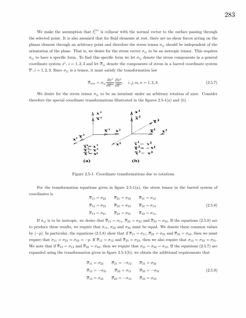
We desire for the stress tensor σij to be an invariant under an arbitrary rotation of axes. Consider
therefore the special coordinate transformations illustrated in the figures 2.5-1(a) and (b).
Figure 2.5-1. Coordinate transformations due to rotations
For the transformation equations given in figure 2.5-1(a), the stress tensor in the barred system of
coordinates isσ11 = σ22 σ21 = σ32 σ31 = σ12
σ12 = σ23 σ22 = σ33 σ32 = σ13
σ13 = σ21 σ23 = σ31 σ33 = σ11.
(2.5.8)
If σij is to be isotropic, we desire that σ11 = σ11, σ22 = σ22 and σ33 = σ33. If the equations (2.5.8) are
to produce these results, we require that σ11, σ22 and σ33 must be equal. We denote these common values
by (−p). In particular, the equations (2.5.8) show that if σ11 = σ11, σ22 = σ22 and σ33 = σ33, then we must
require that σ11 = σ22 = σ33 = −p. If σ12 = σ12 and σ23 = σ23, then we also require that σ12 = σ23 = σ31.
We note that if σ13 = σ13 and σ32 = σ32, then we require that σ21 = σ32 = σ13. If the equations (2.5.7) are
expanded using the transformation given in figure 2.5-1(b), we obtain the additional requirements that
σ11 = σ22 σ21 = −σ12 σ31 = σ32
σ12 = −σ21 σ22 = σ11 σ32 = −σ31
σ13 = σ23 σ23 = −σ13 σ33 = σ33.
(2.5.9)
284
Analysis of these equations implies that if σij is to be isotropic, then σ21 = σ21 = −σ12 = −σ21
or σ21 = 0 which implies σ12 = σ23 = σ31 = σ21 = σ32 = σ13 = 0. (2.5.10)
The above analysis demonstrates that if the stress tensor σij is to be isotropic, it must have the form
σij = −pδij . (2.5.11)
Use the traction condition (2.3.11), and express the stress vector as
t(n)j = σijni = −pnj. (2.5.12)
This equation is interpreted as representing the stress vector at a point on a surface with outward unit
normal ni, where p is the pressure (hydrostatic pressure) stress magnitude assumed to be positive. The
negative sign in equation (2.5.12) denotes a compressive stress.
Imagine a submerged object in a fluid medium. We further imagine the object to be covered with unit
normal vectors emanating from each point on its surface. The equation (2.5.12) shows that the hydrostatic
pressure always acts on the object in a compressive manner. A force results from the stress vector acting on
the object. The direction of the force is opposite to the direction of the unit outward normal vectors. It is
a compressive force at each point on the surface of the object.
The above considerations were for a fluid at rest (hydrostatics). For a fluid in motion (hydrodynamics)
a different set of assumptions must be made. Hydrodynamical experiments show that the shear stress
components are not zero and so we assume a stress tensor having the form
σij = −pδij + τij , i, j = 1, 2, 3, (2.5.13)
where τij is called the viscous stress tensor. Note that all real fluids are both viscous and compressible.
Definition: (Viscous/inviscid fluid) If the viscous stress ten-
sor τij is zero for all i, j, then the fluid is called an inviscid, non-
viscous, ideal or perfect fluid. The fluid is called viscous when τij
is different from zero.
In these notes it is assumed that the equation (2.5.13) represents the basic form for constitutive equations
describing fluid motion.
285
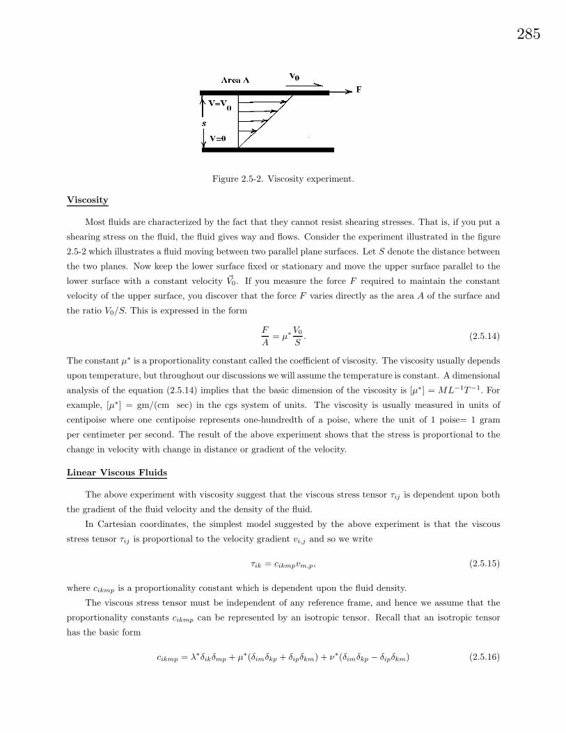
Figure 2.5-2. Viscosity experiment.
Viscosity
Most fluids are characterized by the fact that they cannot resist shearing stresses. That is, if you put a
shearing stress on the fluid, the fluid gives way and flows. Consider the experiment illustrated in the figure
2.5-2 which illustrates a fluid moving between two parallel plane surfaces. Let S denote the distance between
the two planes. Now keep the lower surface fixed or stationary and move the upper surface parallel to the
lower surface with a constant velocity ~V0. If you measure the force F required to maintain the constant
velocity of the upper surface, you discover that the force F varies directly as the area A of the surface and
the ratio V0/S. This is expressed in the form
F
A= µ∗
V0
S. (2.5.14)
The constant µ∗ is a proportionality constant called the coefficient of viscosity. The viscosity usually depends
upon temperature, but throughout our discussions we will assume the temperature is constant. A dimensional
analysis of the equation (2.5.14) implies that the basic dimension of the viscosity is [µ∗] = ML−1T−1. For
example, [µ∗] = gm/(cm sec) in the cgs system of units. The viscosity is usually measured in units of
centipoise where one centipoise represents one-hundredth of a poise, where the unit of 1 poise= 1 gram
per centimeter per second. The result of the above experiment shows that the stress is proportional to the
change in velocity with change in distance or gradient of the velocity.
Linear Viscous Fluids
The above experiment with viscosity suggest that the viscous stress tensor τij is dependent upon both
the gradient of the fluid velocity and the density of the fluid.
In Cartesian coordinates, the simplest model suggested by the above experiment is that the viscous
stress tensor τij is proportional to the velocity gradient vi,j and so we write
τik = cikmpvm,p, (2.5.15)
where cikmp is a proportionality constant which is dependent upon the fluid density.
The viscous stress tensor must be independent of any reference frame, and hence we assume that the
proportionality constants cikmp can be represented by an isotropic tensor. Recall that an isotropic tensor
has the basic form
cikmp = λ∗δikδmp + µ∗(δimδkp + δipδkm) + ν∗(δimδkp − δipδkm) (2.5.16)
286
where λ∗, µ∗ and ν∗ are constants. Examining the results from equations (2.5.11) and (2.5.13) we find that if
the viscous stress is symmetric, then τij = τji. This requires ν∗ be chosen as zero. Consequently, the viscous
stress tensor reduces to the form
τik = λ∗δikvp,p + µ∗(vk,i + vi,k). (2.5.17)
The coefficient µ∗ is called the first coefficient of viscosity and the coefficient λ∗ is called the second coefficient
of viscosity. Sometimes it is convenient to define
ζ = λ∗ +23µ∗ (2.5.18)
as “another second coefficient of viscosity,” or “bulk coefficient of viscosity.” The condition of zero bulk
viscosity is known as Stokes hypothesis. Many fluids problems assume the Stoke’s hypothesis. This requires
that the bulk coefficient be zero or very small. Under these circumstances the second coefficient of viscosity
is related to the first coefficient of viscosity by the relation λ∗ = − 23µ
∗. In the study of shock waves and
acoustic waves the Stoke’s hypothesis is not applicable.
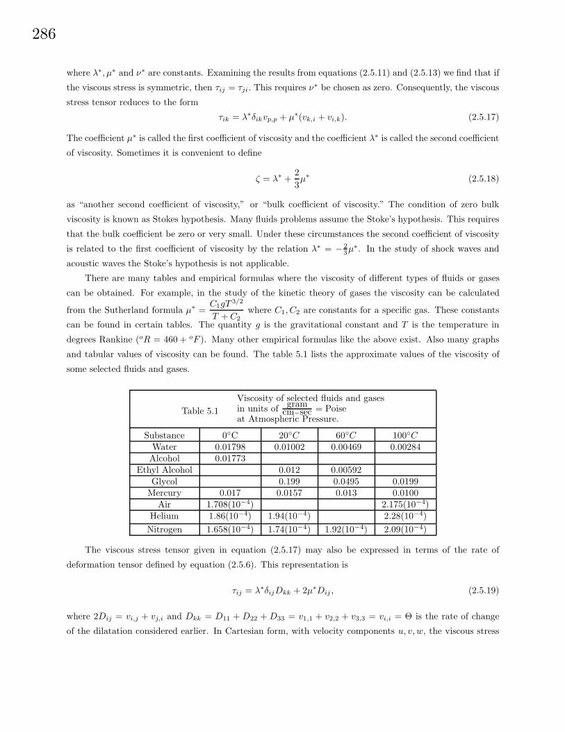
There are many tables and empirical formulas where the viscosity of different types of fluids or gases
can be obtained. For example, in the study of the kinetic theory of gases the viscosity can be calculated
from the Sutherland formula µ∗ =C1gT
3/2
T + C2where C1, C2 are constants for a specific gas. These constants
can be found in certain tables. The quantity g is the gravitational constant and T is the temperature in
degrees Rankine (oR = 460 + oF ). Many other empirical formulas like the above exist. Also many graphs
and tabular values of viscosity can be found. The table 5.1 lists the approximate values of the viscosity of
some selected fluids and gases.
Table 5.1Viscosity of selected fluids and gasesin units of gram
cm−sec = Poiseat Atmospheric Pressure.
Substance 0C 20C 60C 100CWater 0.01798 0.01002 0.00469 0.00284Alcohol 0.01773
Ethyl Alcohol 0.012 0.00592Glycol 0.199 0.0495 0.0199
Mercury 0.017 0.0157 0.013 0.0100Air 1.708(10−4) 2.175(10−4)
Helium 1.86(10−4) 1.94(10−4) 2.28(10−4)Nitrogen 1.658(10−4) 1.74(10−4) 1.92(10−4) 2.09(10−4)
The viscous stress tensor given in equation (2.5.17) may also be expressed in terms of the rate of
deformation tensor defined by equation (2.5.6). This representation is
τij = λ∗δijDkk + 2µ∗Dij , (2.5.19)
where 2Dij = vi,j + vj,i and Dkk = D11 + D22 +D33 = v1,1 + v2,2 + v3,3 = vi,i = Θ is the rate of change
of the dilatation considered earlier. In Cartesian form, with velocity components u, v, w, the viscous stress
287
tensor components are
τxx =(λ∗ + 2µ∗)∂u
∂x+ λ∗
(∂v
∂y+
∂w
∂z
)τyy =(λ∗ + 2µ∗)
∂v
∂y+ λ∗
(∂u
∂x+
∂w
∂z
)τzz =(λ∗ + 2µ∗)
∂w
∂z+ λ∗
(∂u
∂x+
∂v
∂y
)τyx = τxy =µ∗
(∂u
∂y+
∂v
∂x
)τzx = τxz =µ∗
(∂w
∂x+
∂u
∂z
)τzy = τyz =µ∗
(∂v
∂z+
∂w
∂y
)In cylindrical form, with velocity components vr, vθ, vz, the viscous stess tensor components are
τrr =2µ∗ ∂vr
∂r+ λ∗∇ · ~V
τθθ =2µ∗(
1
r
∂vθ
∂θ+
vr
r
)+ λ∗∇ · ~V
τzz =2µ∗ ∂vz
∂z+ λ∗∇ · ~V
where ∇ · ~V =1
r
∂
∂r(rvr) +
1
r
∂vθ
∂θ+
∂vz
∂z
τθr = τrθ =µ∗(
1
r
∂vr
∂θ+
∂vθ
∂r− vθ
r
)τrz = τzr =µ∗
(∂vr
∂z+
∂vz
∂r
)τzθ = τθz =µ∗
(1
r
∂vz
∂θ+
∂vθ
∂z
)In spherical coordinates, with velocity components vρ, vθ, vφ, the viscous stress tensor components have the
form
τρρ =2µ∗ ∂vρ
∂ρ+ λ∗∇ · ~V
τθθ =2µ∗(
1
ρ
∂vθ
∂θ+
vρ
ρ
)+ λ∗∇ · ~V
τφφ =2µ∗(
1
ρ sin θ
∂vφ
∂φ+
vρ
ρ+
vθ cot θ
ρ
)+ λ∗∇ · ~V
where ∇ · ~V =1
ρ2
∂
∂ρ
(ρ2vρ
)+
1
ρ sin θ
∂
∂θ(sin θvθ) +
1
ρ sin θ
∂vφ
∂φ
τρθ = τθρ =µ∗(
ρ∂
∂ρ
(vθ
ρ
)+
1
ρ
∂vρ
∂θ
)τφρ = τρφ =µ∗
(1
ρ sin θ
∂vr
∂φ+ ρ
∂
∂ρ
(vθ
ρ
))τθφ = τφθ =µ∗
(sin θ
ρ
∂
∂θ
(vφ
sin θ
)+
1
ρ sin θ
∂vθ
∂φ
)
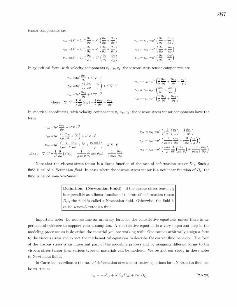
Note that the viscous stress tensor is a linear function of the rate of deformation tensor Dij . Such a
fluid is called a Newtonian fluid. In cases where the viscous stress tensor is a nonlinear function of Dij the
fluid is called non-Newtonian.
Definition: (Newtonian Fluid) If the viscous stress tensor τijis expressible as a linear function of the rate of deformation tensor
Dij , the fluid is called a Newtonian fluid. Otherwise, the fluid is
called a non-Newtonian fluid.
Important note: Do not assume an arbitrary form for the constitutive equations unless there is ex-
perimental evidence to support your assumption. A constitutive equation is a very important step in the
modeling processes as it describes the material you are working with. One cannot arbitrarily assign a form
to the viscous stress and expect the mathematical equations to describe the correct fluid behavior. The form
of the viscous stress is an important part of the modeling process and by assigning different forms to the
viscous stress tensor then various types of materials can be modeled. We restrict our study in these notes
to Newtonian fluids.
In Cartesian coordinates the rate of deformation-stress constitutive equations for a Newtonian fluid can
be written as
σij = −pδij + λ∗δijDkk + 2µ∗Dij (2.5.20)
288
which can also be written in the alternative form
σij = −pδij + λ∗δijvk,k + µ∗(vi,j + vj,i) (2.5.21)
involving the gradient of the velocity.
Upon transforming from a Cartesian coordinate system yi, i = 1, 2, 3 to a more general system of
coordinates xi, i = 1, 2, 3, we write
σmn = σij∂yi
∂xm
∂yj
∂xn . (2.5.22)
Now using the divergence from equation (2.1.3) and substituting equation (2.5.21) into equation (2.5.22) we
obtain a more general expression for the constitutive equation. Performing the indicated substitutions there
results
σmn =[−pδij + λ∗δijvk
,k + µ∗(vi,j + vj,i)] ∂yi
∂xm
∂yj
∂xn
σmn = −pgmn + λ∗gmnvk,k + µ∗(vm,n + vn,m).
Dropping the bar notation, the stress-velocity strain relationships in the general coordinates xi, i = 1, 2, 3, is
σmn = −pgmn + λ∗gmngikvi,k + µ∗(vm,n + vn,m). (2.5.23)
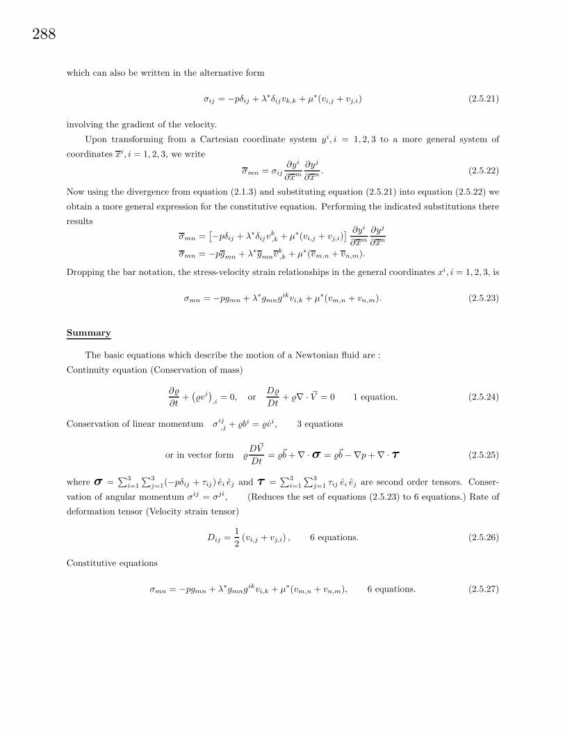
Summary
The basic equations which describe the motion of a Newtonian fluid are :
Continuity equation (Conservation of mass)
∂%
∂t+(%vi),i
= 0, orD%
Dt+ %∇ · ~V = 0 1 equation. (2.5.24)
Conservation of linear momentum σij,j + %bi = %vi, 3 equations
or in vector form %D~V
Dt= %~b+∇ ·σ = %~b−∇p+∇ ·τ (2.5.25)
where σ =∑3
i=1
∑3j=1(−pδij + τij) ei ej and τ =
∑3i=1
∑3j=1 τij ei ej are second order tensors. Conser-
vation of angular momentum σij = σji, (Reduces the set of equations (2.5.23) to 6 equations.) Rate of
deformation tensor (Velocity strain tensor)
Dij =12
(vi,j + vj,i) , 6 equations. (2.5.26)
Constitutive equations
σmn = −pgmn + λ∗gmngikvi,k + µ∗(vm,n + vn,m), 6 equations. (2.5.27)
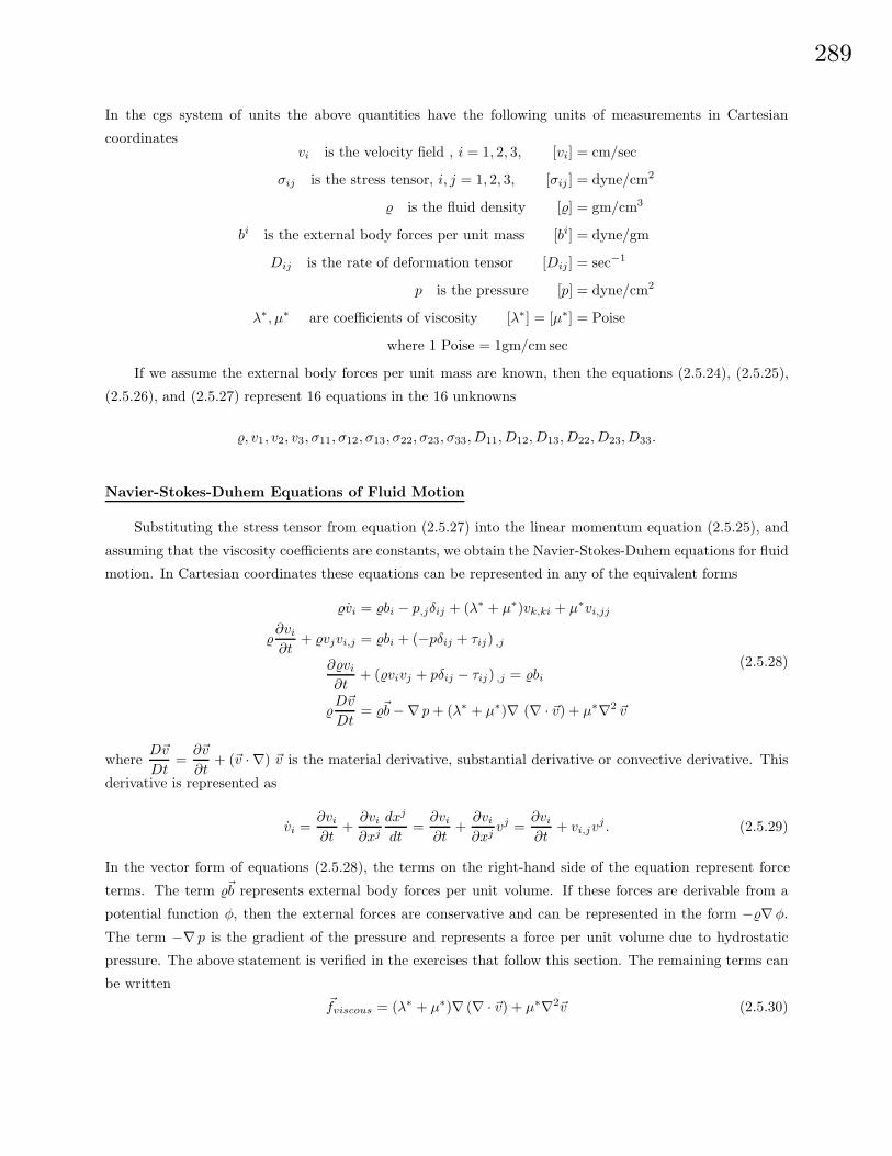
289
In the cgs system of units the above quantities have the following units of measurements in Cartesian
coordinatesvi is the velocity field , i = 1, 2, 3, [vi] = cm/sec
σij is the stress tensor, i, j = 1, 2, 3, [σij ] = dyne/cm2
% is the fluid density [%] = gm/cm3
bi is the external body forces per unit mass [bi] = dyne/gm
Dij is the rate of deformation tensor [Dij ] = sec−1
p is the pressure [p] = dyne/cm2
λ∗, µ∗ are coefficients of viscosity [λ∗] = [µ∗] = Poise
where 1 Poise = 1gm/cmsec
If we assume the external body forces per unit mass are known, then the equations (2.5.24), (2.5.25),
(2.5.26), and (2.5.27) represent 16 equations in the 16 unknowns
%, v1, v2, v3, σ11, σ12, σ13, σ22, σ23, σ33, D11, D12, D13, D22, D23, D33.
Navier-Stokes-Duhem Equations of Fluid Motion
Substituting the stress tensor from equation (2.5.27) into the linear momentum equation (2.5.25), and
assuming that the viscosity coefficients are constants, we obtain the Navier-Stokes-Duhem equations for fluid
motion. In Cartesian coordinates these equations can be represented in any of the equivalent forms
%vi = %bi − p,jδij + (λ∗ + µ∗)vk,ki + µ∗vi,jj
%∂vi
∂t+ %vjvi,j = %bi + (−pδij + τij) ,j
∂%vi
∂t+ (%vivj + pδij − τij) ,j = %bi
%D~v
Dt= %~b−∇ p+ (λ∗ + µ∗)∇ (∇ · ~v) + µ∗∇2 ~v
(2.5.28)
whereD~v
Dt=∂~v
∂t+ (~v · ∇) ~v is the material derivative, substantial derivative or convective derivative. This
derivative is represented as
vi =∂vi
∂t+∂vi
∂xj
dxj
dt=∂vi
∂t+∂vi
∂xjvj =
∂vi
∂t+ vi,jv
j . (2.5.29)
In the vector form of equations (2.5.28), the terms on the right-hand side of the equation represent force
terms. The term %~b represents external body forces per unit volume. If these forces are derivable from a
potential function φ, then the external forces are conservative and can be represented in the form −%∇φ.
The term −∇ p is the gradient of the pressure and represents a force per unit volume due to hydrostatic
pressure. The above statement is verified in the exercises that follow this section. The remaining terms can
be written~fviscous = (λ∗ + µ∗)∇ (∇ · ~v) + µ∗∇2~v (2.5.30)
290
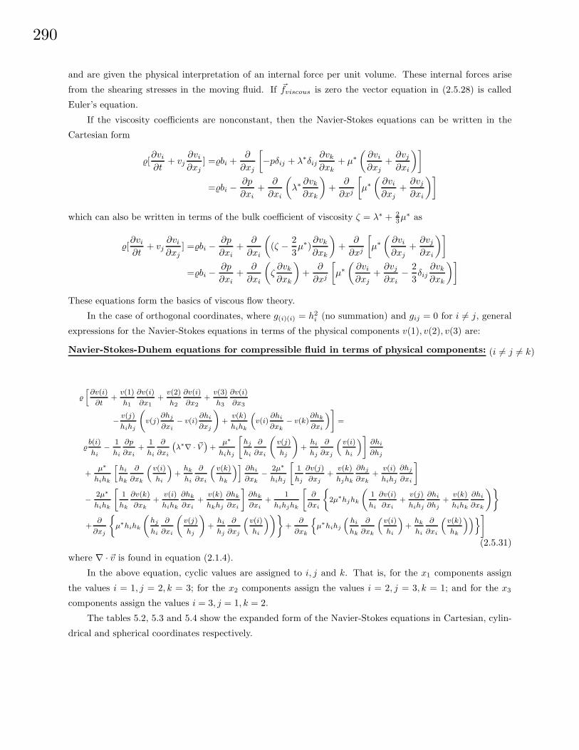
and are given the physical interpretation of an internal force per unit volume. These internal forces arise
from the shearing stresses in the moving fluid. If ~fviscous is zero the vector equation in (2.5.28) is called
Euler’s equation.
If the viscosity coefficients are nonconstant, then the Navier-Stokes equations can be written in the
Cartesian form
%[∂vi
∂t+ vj
∂vi
∂xj] =%bi +
∂
∂xj
[−pδij + λ∗δij
∂vk
∂xk+ µ∗
(∂vi
∂xj+∂vj
∂xi
)]=%bi − ∂p
∂xi+
∂
∂xi
(λ∗∂vk
∂xk
)+
∂
∂xj
[µ∗(∂vi
∂xj+∂vj
∂xi
)]which can also be written in terms of the bulk coefficient of viscosity ζ = λ∗ + 2
3µ∗ as
%[∂vi
∂t+ vj
∂vi
∂xj] =%bi − ∂p
∂xi+
∂
∂xi
((ζ − 2
3µ∗)
∂vk
∂xk
)+
∂
∂xj
[µ∗(∂vi
∂xj+∂vj
∂xi
)]=%bi − ∂p
∂xi+
∂
∂xi
(ζ∂vk
∂xk
)+
∂
∂xj
[µ∗(∂vi
∂xj+∂vj
∂xi− 2
3δij
∂vk
∂xk
)]These equations form the basics of viscous flow theory.
In the case of orthogonal coordinates, where g(i)(i) = h2i (no summation) and gij = 0 for i 6= j, general
expressions for the Navier-Stokes equations in terms of the physical components v(1), v(2), v(3) are:
Navier-Stokes-Duhem equations for compressible fluid in terms of physical components: (i 6= j 6= k)
%
[∂v(i)
∂t+
v(1)
h1
∂v(i)
∂x1+
v(2)
h2
∂v(i)
∂x2+
v(3)
h3
∂v(i)
∂x3
− v(j)
hihj
(v(j)
∂hj
∂xi− v(i)
∂hi
∂xj
)+
v(k)
hihk
(v(i)
∂hi
∂xk− v(k)
∂hk
∂xi
)]=
%b(i)
hi− 1
hi
∂p
∂xi+
1
hi
∂
∂xi
(λ∗∇ · ~V
)+
µ∗
hihj
[hj
hi
∂
∂xi
(v(j)
hj
)+
hi
hj
∂
∂xj
(v(i)
hi
)]∂hi
∂hj
+µ∗
hihk
[hi
hk
∂
∂xk
(v(i)
hi
)+
hk
hi
∂
∂xi
(v(k)
hk
)]∂hi
∂xk− 2µ∗
hihj
[1
hj
∂v(j)
∂xj+
v(k)
hjhk
∂hj
∂xk+
v(i)
hihj
∂hj
∂xi
]− 2µ∗
hihk
[1
hk
∂v(k)
∂xk+
v(i)
hihk
∂hk
∂xi+
v(k)
hkhj
∂hk
∂xi
]∂hk
∂xi+
1
hihjhk
[∂
∂xi
2µ∗hjhk
(1
hi
∂v(i)
∂xi+
v(j)
hihj
∂hi
∂hj+
v(k)
hihk
∂hi
∂xk
)+
∂
∂xj
µ∗hihk
(hj
hi
∂
∂xi
(v(j)
hj
)+
hi
hj
∂
∂xj
(v(i)
hi
))+
∂
∂xk
µ∗hihj
(hi
hk
∂
∂xk
(v(i)
hi
)+
hk
hi
∂
∂xi
(v(k)
hk
))](2.5.31)
where ∇ · ~v is found in equation (2.1.4).
In the above equation, cyclic values are assigned to i, j and k. That is, for the x1 components assign
the values i = 1, j = 2, k = 3; for the x2 components assign the values i = 2, j = 3, k = 1; and for the x3
components assign the values i = 3, j = 1, k = 2.
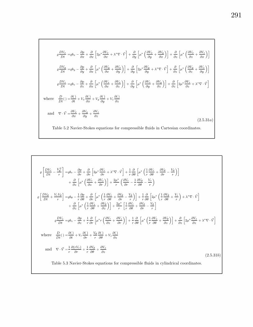
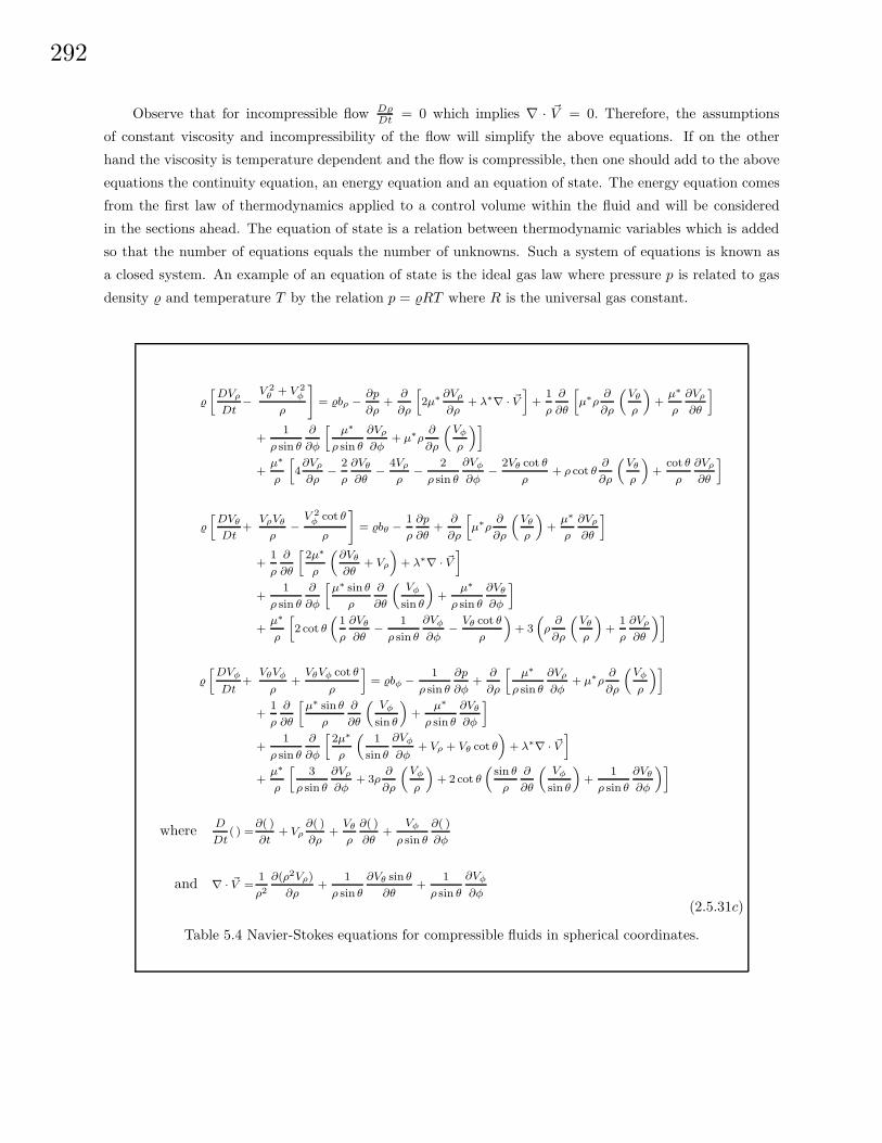
The tables 5.2, 5.3 and 5.4 show the expanded form of the Navier-Stokes equations in Cartesian, cylin-
drical and spherical coordinates respectively.
291
%DVx
Dt=%bx − ∂p
∂x+
∂
∂x
[2µ∗ ∂Vx
∂x+ λ∗∇ · ~V
]+
∂
∂y
[µ∗(
∂Vx
∂y+
∂Vy
∂x
)]+
∂
∂z
[µ∗(
∂Vx
∂z+
∂Vz
∂x
)]
%DVy
Dt=%by − ∂p
∂y+
∂
∂x
[µ∗(
∂Vy
∂x+
∂Vx
∂y
)]+
∂
∂y
[2µ∗ ∂Vy
∂y+ λ∗∇ · ~V
]+
∂
∂z
[µ∗(
∂Vy
∂z+
∂Vz
∂y
)]
%DVz
Dt=%bz − ∂p
∂z+
∂
∂x
[µ∗(
∂Vz
∂x+
∂Vx
∂z
)]+
∂
∂y
[µ∗(
∂Vz
∂y+
∂Vy
∂z
)]+
∂
∂z
[2µ∗ ∂Vz
∂z+ λ∗∇ · ~V
]
where D
Dt( ) =
∂( )
∂t+ Vx
∂( )
∂x+ Vy
∂( )
∂y+ Vz
∂( )
∂z
and ∇ · ~V =∂Vx
∂x+
∂Vy
∂y+
∂Vz
∂z(2.5.31a)
Table 5.2 Navier-Stokes equations for compressible fluids in Cartesian coordinates.
%
[DVr
Dt− V 2
θ
r
]=%br − ∂p
∂r+
∂
∂r
[2µ∗ ∂Vr
∂r+ λ∗∇ · ~V
]+
1
r
∂
∂θ
[µ∗(
1
r
∂Vr
∂θ+
∂Vθ
∂r− Vθ
r
)]+
∂
∂z
[µ∗(
∂Vr
∂z+
∂Vz
∂r
)]+
2µ∗
r
(∂Vr
∂r− 1
r
∂Vθ
∂θ− Vr
r
)%
[DVθ
Dt+
VrVθ
r
]=%bθ −
1
r
∂p
∂θ+
∂
∂r
[µ∗(
1
r
∂Vr
∂θ+
∂Vθ
∂r− Vθ
r
)]+
1
r
∂
∂θ
[2µ∗(
1
r
∂Vθ
∂θ+
Vr
r
)+ λ∗∇ · ~V
]+
∂
∂z
[µ∗(
1
r
∂Vz
∂θ+
∂Vθ
∂z
)]+
2µ∗
r
[1
r
∂Vr
∂θ+
∂Vθ
∂r− Vθ
r
]%
DVz
Dt=%bz − ∂p
∂z+
1
r
∂
∂r
[µ∗r
(∂Vr
∂z+
∂Vz
∂r
)]+
1
r
∂
∂θ
[µ∗(
1
r
∂Vz
∂θ+
∂Vθ
∂z
)]+
∂
∂z
[2µ∗ ∂Vz
∂z+ λ∗∇ · ~V
]
where D
Dt( ) =
∂( )
∂t+ Vr
∂( )
∂r+
Vθ
r
∂( )
∂θ+ Vz
∂( )
∂z
and ∇ · ~V =1
r
∂(rVr)
∂r+
1
r
∂Vθ
∂θ+
∂Vz
∂z(2.5.31b)
Table 5.3 Navier-Stokes equations for compressible fluids in cylindrical coordinates.
292
Observe that for incompressible flow D%Dt = 0 which implies ∇ · ~V = 0. Therefore, the assumptions
of constant viscosity and incompressibility of the flow will simplify the above equations. If on the other
hand the viscosity is temperature dependent and the flow is compressible, then one should add to the above
equations the continuity equation, an energy equation and an equation of state. The energy equation comes
from the first law of thermodynamics applied to a control volume within the fluid and will be considered
in the sections ahead. The equation of state is a relation between thermodynamic variables which is added
so that the number of equations equals the number of unknowns. Such a system of equations is known as
a closed system. An example of an equation of state is the ideal gas law where pressure p is related to gas
density % and temperature T by the relation p = %RT where R is the universal gas constant.
%
[DVρ
Dt−
V 2θ + V 2
φ
ρ
]= %bρ − ∂p
∂ρ+
∂
∂ρ
[2µ∗ ∂Vρ
∂ρ+ λ∗∇ · ~V
]+
1
ρ
∂
∂θ
[µ∗ρ
∂
∂ρ
(Vθ
ρ
)+
µ∗
ρ
∂Vρ
∂θ
]+
1
ρ sin θ
∂
∂φ
[µ∗
ρ sin θ
∂Vρ
∂φ+ µ∗ρ
∂
∂ρ
(Vφ
ρ
)]+
µ∗
ρ
[4
∂Vρ
∂ρ− 2
ρ
∂Vθ
∂θ− 4Vρ
ρ− 2
ρ sin θ
∂Vφ
∂φ− 2Vθ cot θ
ρ+ ρ cot θ
∂
∂ρ
(Vθ
ρ
)+
cot θ
ρ
∂Vρ
∂θ
]
%
[DVθ
Dt+
VρVθ
ρ−
V 2φ cot θ
ρ
]= %bθ −
1
ρ
∂p
∂θ+
∂
∂ρ
[µ∗ρ
∂
∂ρ
(Vθ
ρ
)+
µ∗
ρ
∂Vρ
∂θ
]+
1
ρ
∂
∂θ
[2µ∗
ρ
(∂Vθ
∂θ+ Vρ
)+ λ∗∇ · ~V
]+
1
ρ sin θ
∂
∂φ
[µ∗ sin θ
ρ
∂
∂θ
(Vφ
sin θ
)+
µ∗
ρ sin θ
∂Vθ
∂φ
]+
µ∗
ρ
[2 cot θ
(1
ρ
∂Vθ
∂θ− 1
ρ sin θ
∂Vφ
∂φ− Vθ cot θ
ρ
)+ 3
(ρ
∂
∂ρ
(Vθ
ρ
)+
1
ρ
∂Vρ
∂θ
)]
%
[DVφ
Dt+
VθVφ
ρ+
VθVφ cot θ
ρ
]= %bφ −
1
ρ sin θ
∂p
∂φ+
∂
∂ρ
[µ∗
ρ sin θ
∂Vρ
∂φ+ µ∗ρ
∂
∂ρ
(Vφ
ρ
)]+
1
ρ
∂
∂θ
[µ∗ sin θ
ρ
∂
∂θ
(Vφ
sin θ
)+
µ∗
ρ sin θ
∂Vθ
∂φ
]+
1
ρ sin θ
∂
∂φ
[2µ∗
ρ
(1
sin θ
∂Vφ
∂φ+ Vρ + Vθ cot θ
)+ λ∗∇ · ~V
]+
µ∗
ρ
[3
ρ sin θ
∂Vρ
∂φ+ 3ρ
∂
∂ρ
(Vφ
ρ
)+ 2 cot θ
(sin θ
ρ
∂
∂θ
(Vφ
sin θ
)+
1
ρ sin θ
∂Vθ
∂φ
)]
where D
Dt( ) =
∂( )
∂t+ Vρ
∂( )
∂ρ+
Vθ
ρ
∂( )
∂θ+
Vφ
ρ sin θ
∂( )
∂φ
and ∇ · ~V =1
ρ2
∂(ρ2Vρ)
∂ρ+
1
ρ sin θ
∂Vθ sin θ
∂θ+
1
ρ sin θ
∂Vφ
∂φ(2.5.31c)
Table 5.4 Navier-Stokes equations for compressible fluids in spherical coordinates.
293
We now consider various special cases of the Navier-Stokes-Duhem equations.Special Case 1: Assume that ~b is a conservative force such that ~b = −∇φ. Also assume that the viscous
force terms are zero. Consider steady flow (∂~v∂t = 0) and show that equation (2.5.28) reduces to the equation
(~v · ∇)~v =−1%∇ p−∇φ % is constant. (2.5.32)
Employing the vector identity
(~v · ∇)~v = (∇× ~v)× ~v +12∇(~v · ~v), (2.5.33)
we take the dot product of equation (2.5.32) with the vector ~v. Noting that ~v · [(∇× ~v)× ~v] = ~0 we obtain
~v · ∇[p
%+ φ+
12v2
]= 0. (2.5.34)
This equation shows that for steady flow we will have
p
%+ φ+
12v2 = constant (2.5.35)
along a streamline. This result is known as Bernoulli’s theorem. In the special case where φ = gh is a
force due to gravity, the equation (2.5.35) reduces top
%+v2
2+ gh = constant. This equation is known as
Bernoulli’s equation. It is a conservation of energy statement which has many applications in fluids.
Special Case 2: Assume that ~b = −∇φ is conservative and define the quantity Ω by
~Ω = ∇ × ~v = curl~v ω =12Ω (2.5.36)
as the vorticity vector associated with the fluid flow and observe that its magnitude is equivalent to twice
the angular velocity of a fluid particle. Then using the identity from equation (2.5.33) we can write the
Navier-Stokes-Duhem equations in terms of the vorticity vector. We obtain the hydrodynamic equations
∂~v
∂t+ ~Ω× ~v +
12∇ v2 = −1
%∇ p−∇φ+
1%~fviscous, (2.5.37)
where ~fviscous is defined by equation (2.5.30). In the special case of nonviscous flow this further reduces to
the Euler equation∂~v
∂t+ ~Ω× ~v +
12∇ v2 = −1
%∇ p−∇φ.
If the density % is a function of the pressure only it is customary to introduce the function
P =∫ p
c
dp
%so that ∇P =
dP
dp∇p =
1%∇p
then the Euler equation becomes
∂~v
∂t+ ~Ω× ~v = −∇(P + φ+
12v2).
Some examples of vorticies are smoke rings, hurricanes, tornadoes, and some sun spots. You can create
a vortex by letting water stand in a sink and then remove the plug. Watch the water and you will see that
a rotation or vortex begins to occur. Vortices are associated with circulating motion.
294
Pick an arbitrary simple closed curve C and place it in the fluid flow and define the line integral
K =∮
C
~v · et ds, where ds is an element of arc length along the curve C, ~v is the vector field defining the
velocity, and et is a unit tangent vector to the curve C. The integral K is called the circulation of the fluid
around the closed curve C. The circulation is the summation of the tangential components of the velocity
field along the curve C. The local vorticity at a point is defined as the limit
limArea→0
Circulation around CArea inside C
= circulation per unit area.
By Stokes theorem, if curl~v = ~0, then the fluid is called irrotational and the circulation is zero. Otherwise
the fluid is rotational and possesses vorticity.
If we are only interested in the velocity field we can eliminate the pressure by taking the curl of both
sides of the equation (2.5.37). If we further assume that the fluid is incompressible we obtain the special
equations∇ · ~v = 0 Incompressible fluid, % is constant.
~Ω = curl~v Definition of vorticity vector.
∂~Ω∂t
+∇× (~Ω× ~v) =µ∗
%∇2~Ω Results because curl of gradient is zero.
(2.5.38)
Note that when Ω is identically zero, we have irrotational motion and the above equations reduce to the
Cauchy-Riemann equations. Note also that if the term ∇× (~Ω × ~v) is neglected, then the last equation in
equation (2.5.38) reduces to a diffusion equation. This suggests that the vorticity diffuses through the fluid
once it is created.
Vorticity can be caused by a rigid rotation or by shear flow. For example, in cylindrical coordinates let~V = rω eθ, with r, ω constants, denote a rotational motion, then curl ~V = ∇× ~V = 2ω ez, which shows the
vorticity is twice the rotation vector. Shear can also produce vorticity. For example, consider the velocity
field ~V = y e1 with y ≥ 0. Observe that this type of flow produces shear because |~V | increases as y increases.
For this flow field we have curl ~V = ∇× ~V = − e3. The right-hand rule tells us that if an imaginary paddle
wheel is placed in the flow it would rotate clockwise because of the shear effects.
Scaled Variables
In the Navier-Stokes-Duhem equations for fluid flow we make the assumption that the external body
forces are derivable from a potential function φ and write ~b = −∇φ [dyne/gm] We also want to write the
Navier-Stokes equations in terms of scaled variables
~v =~v
v0
p =p
p0
% =%
%0
t =t
τ
φ =φ
gL,
x =x
L
y =y
L
z =z
L
which can be referred to as the barred system of dimensionless variables. Dimensionless variables are intro-
duced by scaling each variable associated with a set of equations by an appropriate constant term called a
characteristic constant associated with that variable. Usually the characteristic constants are chosen from
various parameters used in the formulation of the set of equations. The characteristic constants assigned to
each variable are not unique and so problems can be scaled in a variety of ways. The characteristic constants
295
assigned to each variable are scales, of the appropriate dimension, which act as reference quantities which
reflect the order of magnitude changes expected of that variable over a certain range or area of interest
associated with the problem. An inappropriate magnitude selected for a characteristic constant can result
in a scaling where significant information concerning the problem can be lost. This is analogous to selecting
an inappropriate mesh size in a numerical method. The numerical method might give you an answer but
details of the answer might be lost.
In the above scaling of the variables occurring in the Navier-Stokes equations we let v0 denote some
characteristic speed, p0 a characteristic pressure, %0 a characteristic density, L a characteristic length, g the
acceleration of gravity and τ a characteristic time (for example τ = L/v0), then the barred variables v, p,
%,φ, t, x, y and z are dimensionless. Define the barred gradient operator by
∇ =∂
∂xe1 +
∂
∂ye2 +
∂
∂ze3
where all derivatives are with respect to the barred variables. The above change of variables reduces the
Navier-Stokes-Duhem equations
%∂~v
∂t+ %(~v · ∇)~v = −%∇φ−∇ p+ (λ∗ + µ∗)∇ (∇ · ~v) + µ∗∇2 ~v, (2.5.39)
to the form(%0v0
τ
)%∂~v
∂t+(%0v
20
L
)%(~v · ∇)~v = −%0g%∇φ−
(p0
L
)∇p
+(λ∗ + µ∗)
L2v0∇
(∇ · ~v)+(µ∗v0L2
)∇2~v.
(2.5.40)
Now if each term in the equation (2.5.40) is divided by the coefficient %0v20/L, we obtain the equation
S%∂~v
∂t+ %
(~v · ∇)~v =
−1F%∇φ− E∇p+
(λ∗
µ∗+ 1)
1R∇ (∇ · ~v)+
1R∇2~v (2.5.41)
which has the dimensionless coefficients
E =p0
%0v20
= Euler number
F =v20
gL= Froude number, g is acceleration of gravity
R =%0V0L
µ∗= Reynolds number
S =L
τv0= Strouhal number.
Dropping the bars over the symbols, we write the dimensionless equation using the above coefficients.
The scaled equation is found to have the form
S%∂~v
∂t+ %(~v · ∇)~v = − 1
F%∇φ− E∇p+
(λ∗
µ∗+ 1)
1R∇ (∇ · ~v) +
1R∇2~v (2.5.42)
296
Boundary Conditions
Fluids problems can be classified as internal flows or external flows. An example of an internal flow
problem is that of fluid moving through a converging-diverging nozzle. An example of an external flow
problem is fluid flow around the boundary of an aircraft. For both types of problems there is some sort of
boundary which influences how the fluid behaves. In these types of problems the fluid is assumed to adhere
to a boundary. Let ~rb denote the position vector to a point on a boundary associated with a moving fluid,
and let ~r denote the position vector to a general point in the fluid. Define ~v(~r) as the velocity of the fluid at
the point ~r and define ~v(~rb) as the known velocity of the boundary. The boundary might be moving within
the fluid or it could be fixed in which case the velocity at all points on the boundary is zero. We define the
boundary condition associated with a moving fluid as an adherence boundary condition.
Definition: (Adherence Boundary Condition)
An adherence boundary condition associated with a fluid in motion
is defined as the limit lim~r→~rb
~v(~r) = ~v(~rb) where ~rb is the position
vector to a point on the boundary.
Sometimes, when no finite boundaries are present, it is necessary to impose conditions on the components
of the velocity far from the origin. Such conditions are referred to as boundary conditions at infinity.
Summary and Additional Considerations
Throughout the development of the basic equations of continuum mechanics we have neglected ther-
modynamical and electromagnetic effects. The inclusion of thermodynamics and electromagnetic fields adds
additional terms to the basic equations of a continua. These basic equations describing a continuum are:
Conservation of mass
The conservation of mass is a statement that the total mass of a body is unchanged during its motion.
This is represented by the continuity equation
∂%
∂t+ (%vk),k = 0 or
D%
Dt+ %∇ · ~V = 0
where % is the mass density and vk is the velocity.
Conservation of linear momentum
The conservation of linear momentum requires that the time rate of change of linear momentum equal
the resultant of all forces acting on the body. In symbols, we write
D
Dt
∫V%vi dτ =
∫SF i
(s)ni dS +∫V%F i
(b) dτ +n∑
α=1
F i(α) (2.5.43)
where Dvi
Dt = ∂vi
∂t + ∂vi
∂xk vk is the material derivative, F i
(s) are the surface forces per unit area, F i(b) are the
body forces per unit mass and F i(α) represents isolated external forces. Here S represents the surface and
V represents the volume of the control volume. The right-hand side of this conservation law represents the
resultant force coming from the consideration of all surface forces and body forces acting on a control volume.
297
Surface forces acting upon the control volume involve such things as pressures and viscous forces, while body
forces are due to such things as gravitational, magnetic and electric fields.
Conservation of angular momentum
The conservation of angular momentum states that the time rate of change of angular momentum
(moment of linear momentum) must equal the total moment of all forces and couples acting upon the body.
In symbols,
D
Dt
∫V%eijkx
jvk dτ =∫Seijkx
jF k(s) dS +
∫V%eijkx
jF k(b) dτ +
n∑α=1
(eijkxj(α)F
k(α) +M i
(α)) (2.5.44)
where M i(α) represents concentrated couples and F k
(α) represents isolated forces.
Conservation of energy
The conservation of energy law requires that the time rate of change of kinetic energy plus internal
energies is equal to the sum of the rate of work from all forces and couples plus a summation of all external
energies that enter or leave a control volume per unit of time. The energy equation results from the first law
of thermodynamics and can be written
D
Dt(E +K) = W + Qh (2.5.45)
where E is the internal energy, K is the kinetic energy, W is the rate of work associated with surface and
body forces, and Qh is the input heat rate from surface and internal effects.
Let e denote the internal specific energy density within a control volume, then E =∫V%e dτ represents
the total internal energy of the control volume. The kinetic energy of the control volume is expressed as
K =12
∫V%gijv
ivj dτ where vi is the velocity, % is the density and dτ is a volume element. The energy (rate
of work) associated with the body and surface forces is represented
W =∫SgijF
i(s)v
j dS +∫V%gijF
i(b)v
j dτ +n∑
α=1
(gijFi(α)v
j + gijMi(α)ω
j)
where ωj is the angular velocity of the point xi(α), F
i(α) are isolated forces, and M i
(α) are isolated couples.
Two external energy sources due to thermal sources are heat flow qi and rate of internal heat production ∂Q∂t
per unit volume. The conservation of energy can thus be represented
D
Dt
∫V%(e+
12gijv
ivj) dτ =∫S(gijF
i(s)v
j − qini) dS +
∫V(%gijF
i(b)v
j +∂Q
∂t) dτ
+n∑
α=1
(gijFi(α)v
j + gijMi(α)ω
j + U(α))(2.5.46)
where U(α) represents all other energies resulting from thermal, mechanical, electric, magnetic or chemical
sources which influx the control volume and D/Dt is the material derivative.
In equation (2.5.46) the left hand side is the material derivative of an integral of the total energy
et = %(e + 12gijv
ivj) over the control volume. Material derivatives are not like ordinary derivatives and so
298
we cannot interchange the order of differentiation and integration in this term. Here we must use the result
thatD
Dt
∫Vet dτ =
∫V
(∂et
∂t+∇ · (et
~V ))dτ.
To prove this result we consider a more general problem. Let A denote the amount of some quantity per
unit mass. The quantity A can be a scalar, vector or tensor. The total amount of this quantity inside the
control volume is A =∫V %A dτ and therefore the rate of change of this quantity is
∂A
∂t=∫V
∂(%A)∂t
dτ =D
Dt
∫V%A dτ −
∫S%A~V · n dS,
which represents the rate of change of material within the control volume plus the influx into the control
volume. The minus sign is because n is always a unit outward normal. By converting the surface integral to
a volume integral, by the Gauss divergence theorem, and rearranging terms we find that
D
Dt
∫V%A dτ =
∫V
[∂(%A)∂t
+∇ · (%A~V )]dτ.
In equation (2.5.46) we neglect all isolated external forces and substitute F i(s) = σijnj , F i
(b) = bi where
σij = −pδij + τij . We then replace all surface integrals by volume integrals and find that the conservation of
energy can be represented in the form
∂et
∂t+∇ · (et
~V ) = ∇(σ · ~V )−∇ · ~q + %~b · ~V +∂Q
∂t(2.5.47)
where et = %e+ %(v21 + v2
2 + v23)/2 is the total energy and σ =
∑3i=1
∑3j=1 σij ei ej is the second order stress
tensor. Here
σ · ~V = −p~V +3∑
j=1
τ1jvj e1 +3∑
j=1
τ2jvj e2 +3∑
j=1
τ3jvj e3 = −p~V + τ · ~V
and τij = µ∗(vi,j + vj,i) + λ∗δijvk,k is the viscous stress tensor. Using the identities
%D(et/%)Dt
=∂et
∂t+∇ · (et
~V ) and %D(et/%)Dt
= %De
Dt+ %
D(V 2/2)Dt
together with the momentum equation (2.5.25) dotted with ~V as
%D~V
Dt· ~V = %~b · ~V −∇p · ~V + (∇ ·τ ) · ~V
the energy equation (2.5.47) can then be represented in the form
%D e
Dt+ p(∇ · ~V ) = −∇ · ~q +
∂Q
∂t+ Φ (2.5.48)
where Φ is the dissipation function and can be represented
Φ = (τijvi) ,j − viτij,j = ∇ · (τ · ~V )− (∇ ·τ ) · ~V .
As an exercise it can be shown that the dissipation function can also be represented as Φ = 2µ∗DijDij +λ∗Θ2
where Θ is the dilatation. The heat flow vector is determined from the Fourier law of heat conduction in
299
terms of the temperature T as ~q = −κ∇T , where κ is the thermal conductivity. Consequently, the energy
equation can be written as
%De
Dt+ p(∇ · ~V ) =
∂Q
∂t+ Φ +∇(k∇T ). (2.5.49)
In Cartesian coordinates (x, y, z) we use
D
Dt=∂
∂t+ Vx
∂
∂x+ Vy
∂
∂y+ Vz
∂
∂z
∇ · ~V =∂Vx
∂x+∂Vy
∂y+∂Vz
∂z
∇ · (κ∇T ) =∂
∂x
(κ∂T
∂x
)+
∂
∂y
(κ∂T
∂y
)+
∂
∂z
(κ∂T
∂z
)In cylindrical coordinates (r, θ, z)
D
Dt=∂
∂t+ Vr
∂
∂r+Vθ
r
∂
∂θ+ Vz
∂
∂z
∇ · ~V =1r
∂
∂r(rVr) +
1r2∂Vθ
∂θ+∂Vz
∂z
∇ · (κ∇T ) =1r
∂
∂r
(rκ∂T
∂r
)+
1r2
∂
∂θ
(κ∂T
∂θ
)+
∂
∂z
(κ∂T
∂z
)and in spherical coordinates (ρ, θ, φ)
D
Dt=∂
∂t+ Vρ
∂
∂ρ+Vθ
ρ
∂
∂θ
Vφ
ρ sin θ∂
∂φ
∇ · ~V =1ρ2
∂
∂ρ(ρVρ) +
1ρ sin θ
∂
∂θ(Vθ sin θ) +
1ρ sin θ
∂Vφ
∂φ
∇ · (κ∇T ) =1ρ2
∂
∂ρ
(ρ2κ
∂T
∂ρ
)+
1ρ2 sin θ
∂
∂θ
(κ sin θ
∂T
∂θ
)+
1ρ2 sin2 θ
∂
∂φ
(κ∂T
∂φ
)The combination of terms h = e+ p/% is known as enthalpy and at times is used to express the energy
equation in the form
%D h
Dt=Dp
Dt+∂Q
∂t−∇ · ~q + Φ.
The derivation of this equation is left as an exercise.Conservative Systems
Let Q denote some physical quantity per unit volume. Here Q can be either a scalar, vector or tensor
field. Place within this field an imaginary simple closed surface S which encloses a volume V. The total
amount of Q within the surface is given by∫∫∫
V Qdτ and the rate of change of this amount with respect
to time is ∂∂t
∫∫∫Qdτ. The total amount of Q within S changes due to sources (or sinks) within the volume
and by transport processes. Transport processes introduce a quantity ~J, called current, which represents a
flow per unit area across the surface S. The inward flux of material into the volume is denoted∫∫
S− ~J · n dσ
(n is a unit outward normal.) The sources (or sinks) SQ denotes a generation (or loss) of material per unit
volume so that∫∫∫
VSQ dτ denotes addition (or loss) of material to the volume. For a fixed volume we then
have the material balance ∫∫∫V
∂Q
∂tdτ = −
∫∫S
~J · n dσ +∫∫∫
V
SQ dτ.
300
Using the divergence theorem of Gauss one can derive the general conservation law
∂Q
∂t+∇ · ~J = SQ (2.5.50)
The continuity equation and energy equations are examples of a scalar conservation law in the special case
where SQ = 0. In Cartesian coordinates, we can represent the continuity equation by letting
Q = % and ~J = %~V = %(Vx e1 + Vy e2 + Vz e3) (2.5.51)
The energy equation conservation law is represented by selecting Q = et and neglecting the rate of internal
heat energy we let
~J =
[(et + p)v1 −
3∑i=1
viτxi + qx
]e1+[
(et + p)v2 −3∑
i=1
viτyi + qy
]e2+[
(et + p)v3 −3∑
i=1
viτzi + qz
]e3.
(2.5.52)
In a general orthogonal system of coordinates (x1, x2, x3) the equation (2.5.50) is written
∂
∂t((h1h2h3Q)) +
∂
∂x1((h2h3J1)) +
∂
∂x2((h1h3J2)) +
∂
∂x3((h1h2J3)) = 0,
where h1, h2, h3 are scale factors obtained from the transformation equations to the general orthogonal
coordinates.
The momentum equations are examples of a vector conservation law having the form
∂~a
∂t+∇ · (T ) = %~b (2.5.53)
where ~a is a vector and T is a second order symmetric tensor T =3∑
k=1
3∑j=1
Tjk ej ek. In Cartesian coordinates
we let ~a = %(Vx e1 + Vy e2 + Vz e3) and Tij = %vivj + pδij − τij . In general coordinates (x1, x2, x3) the
momentum equations result by selecting ~a = %~V and Tij = %vivj + pδij − τij . In a general orthogonal system
the conservation law (2.5.53) has the general form
∂
∂t((h1h2h3~a)) +
∂
∂x1
((h2h3T · e1)
)+
∂
∂x2
((h1h3T · e2)
)+
∂
∂x3
((h1h2T · e3)
)= %~b. (2.5.54)
Neglecting body forces and internal heat production, the continuity, momentum and energy equations
can be expressed in the strong conservative form
∂U
∂t+∂E
∂x+∂F
∂y+∂G
∂z= 0 (2.5.55)
where
U =
ρρVx
ρVy
ρVz
et
(2.5.56)
301
E =
ρVx
ρV 2x + p− τxx
ρVxVy − τxy
ρVxVz − τxz
(et + p)Vx − Vxτxx − Vyτxy − Vzτxz + qx
(2.5.57)
F =
ρVy
ρVxVy − τxy
ρV 2y + p− τyy
ρVyVz − τyz
(et + p)Vy − Vxτyx − Vyτyy − Vzτyz + qy
(2.5.58)
G =
ρVz
ρVxVz − τxz
ρVyVz − τyz
ρV 2z + p− τzz
(et + p)Vz − Vxτzx − Vyτzy − Vzτzz + qz
(2.5.59)
where the shear stresses are τij = µ∗(Vi,j + Vj,i) + δijλ∗Vk,k for i, j, k = 1, 2, 3.
Computational Coordinates
To transform the conservative system (2.5.55) from a physical (x, y, z) domain to a computational (ξ, η, ζ)
domain requires that a general change of variables take place. Consider the following general transformation
of the independent variables
ξ = ξ(x, y, z) η = η(x, y, z) ζ = ζ(x, y, z) (2.5.60)
with Jacobian different from zero. The chain rule for changing variables in equation (2.5.55) requires the
operators∂( )∂x
=∂( )∂ξ
ξx +∂( )∂η
ηx +∂( )∂ζ
ζx
∂( )∂y
=∂( )∂ξ
ξy +∂( )∂η
ηy +∂( )∂ζ
ζy
∂( )∂z
=∂( )∂ξ
ξz +∂( )∂η
ηz +∂( )∂ζ
ζz
(2.5.61)
The partial derivatives in these equations occur in the differential expressions
dξ =ξx dx+ ξy dy + ξz dz
dη =ηx dx+ ηy dy + ηz dz
dζ =ζx dx+ ζy dy + ζz dz
or
dξdηdζ
=
ξx ξy ξzηx ηy ηz
ζx ζy ζz
dxdydz
(2.5.62)
In a similar mannaer from the inverse transformation equations
x = x(ξ, η, ζ) y = y(ξ, η, ζ) z = z(ξ, η, ζ) (2.5.63)
we can write the differentials
dx =xξ dξ + xη dη + xζ dζ
dy =yξ dξ + yη dη + yζ dζ
dz =zξ dξ + zζ dζ + zζ dζ
or
dxdydz
=
xξ xη xζ
yξ yη yζ
zξ zη zζ
dξdηdζ
(2.5.64)
302
The transformations (2.5.62) and (2.5.64) are inverses of each other and so we can write ξx ξy ξzηx ηy ηz
ζx ζy ζz
=
xξ xη xζ
yξ yη yζ
zξ zη zζ
−1
=J
yηzζ − yζzη −(xηzζ − xζzη) xηyζ − xζyη
−(yξzζ − yζzξ) xξzζ − xζzξ −(xξyζ − xζyξ)yξzη − yηzξ −(xξzη − xηzξ) xξyη − xηyξ
(2.5.65)
By comparing like elements in equation (2.5.65) we obtain the relations
ξx =J(yηzζ − yζzη)
ξy =− J(xηzζ − xζzη)
ξz =J(xηyζ − xζyη)
ηx =− J(yξzζ − yζzξ)
ηy =J(xξzζ − zζzξ)
ηz =− J(xξyζ − xζyξ)
ζx =J(yξzη − yηzξ)
ζy =− J(xξzη − xηzξ)
ζz =J(xξyη − xηyξ)
(2.5.66)
The equations (2.5.55) can now be written in terms of the new variables (ξ, η, ζ) as
∂U
∂t+∂E
∂ξξx +
∂E
∂ηηx +
∂E
∂ζζx +
∂F
∂ξξy +
∂F
∂ηηy +
∂F
∂ζζy +
∂G
∂ξξz +
∂G
∂ηηz +
∂G
∂ζζz = 0 (2.5.67)
Now divide each term by the Jacobian J and write the equation (2.5.67) in the form
∂
∂t
(U
J
)+
∂
∂ξ
(Eξx + Fξy +Gξz
J
)+
∂
∂η
(Eηx + Fηy +Gηz
J
)+
∂
∂ζ
(Eζx + Fζy +Gζz
J
)− E
∂
∂ξ
(ξxJ
)+
∂
∂η
(ηx
J
)+
∂
∂ζ
(ζxJ
)− F
∂
∂ξ
(ξyJ
)+
∂
∂η
(ηy
J
)+
∂
∂ζ
(ζyJ
)−G
∂
∂ξ
(ξzJ
)+
∂
∂η
(ηz
J
)+
∂
∂ζ
(ζzJ
)= 0
(2.5.68)
Using the relations given in equation (2.5.66) one can show that the curly bracketed terms above are all zero
and so the transformed equations (2.5.55) can also be written in the conservative form
∂U
∂t+∂E
∂ξ+∂F
∂η+∂G
∂ζ= 0 (2.5.69)
whereU =
U
J
E =Eξx + Fξy +Gξz
J
F =Eηx + Fηy +Gηz
J
G =Eζx + Fζy +Gζz
J
(2.5.70)
303
Fourier law of heat conduction
The Fourier law of heat conduction can be written qi = −κT,i for isotropic material and qi = −κijT,j
for anisotropic material. The Prandtl number is a nondimensional constant defined as Pr = cpµ∗
κ so that
the heat flow terms can be represented in Cartesian coordinates as
qx = −cpµ∗
Pr
∂T
∂xqy = −cpµ
∗
Pr
∂T
∂yqz = −cpµ
∗
Pr
∂T
∂z
Now one can employ the equation of state relations P = %e(γ − 1), cp = γRγ−1 , cpT = γRT
γ−1 and write the
above equations in the alternate forms
qx = − µ∗
Pr(γ − 1)∂
∂x
(γP
%
)qy = − µ∗
Pr(γ − 1)∂
∂y
(γP
%
)qz = − µ∗
Pr(γ − 1)∂
∂z
(γP
%
)
The speed of sound is given by a =
√γP
%=√γRT and so one can substitute a2 in place of the ratio
γP
%
in the above equations.
Equilibrium and Nonequilibrium Thermodynamics
High temperature gas flows require special considerations. In particular, the specific heat for monotonic
and diatomic gases are different and are in general a function of temperature. The energy of a gas can be
written as e = et + er + ev + ee + en where et represents translational energy, er is rotational energy, ev is
vibrational energy, ee is electronic energy, and en is nuclear energy. The gases follow a Boltzmann distribution
for each degree of freedom and consequently at very high temperatures the rotational, translational and
vibrational degrees of freedom can each have their own temperature. Under these conditions the gas is said
to be in a state of nonequilibrium. In such a situation one needs additional energy equations. The energy
equation developed in these notes is for equilibrium thermodynamics where the rotational, translational and
vibrational temperatures are the same.
Equation of state
It is assumed that an equation of state such as the universal gas law or perfect gas law pV = nRT
holds which relates pressure p [N/m2], volume V [m3], amount of gas n [mol],and temperature T [K] where
R [J/mol −K] is the universal molar gas constant. If the ideal gas law is represented in the form p = %RT
where % [Kg/m3] is the gas density, then the universal gas constant must be expressed in units of [J/Kg−K]
(See Appendix A). Many gases deviate from this ideal behavior. In order to account for the intermolecular
forces associated with high density gases, an empirical equation of state of the form
p = ρRT +M1∑n=1
βnρn+r1 + e−γ1ρ−γ2ρ2
M2∑n=1
cnρn+r2
involving constants M1,M2, βn, cn, r1, r2, γ1, γ2 is often used. For a perfect gas the relations
e = cvT γ =cpcv
cv =R
γ − 1cp =
γR
γ − 1h = cpT
hold, where R is the universal gas constant, cv is the specific heat at constant volume, cp is the specific
heat at constant pressure, γ is the ratio of specific heats and h is the enthalpy. For cv and cp constants the
relations p = (γ − 1)%e and RT = (γ − 1)e can be verified.
304
EXAMPLE 2.5-1. (One-dimensional fluid flow)
Construct an x-axis running along the center line of a long cylinder with cross sectional areaA. Consider
the motion of a gas driven by a piston and moving with velocity v1 = u in the x-direction. From an Eulerian
point of view we imagine a control volume fixed within the cylinder and assume zero body forces. We require
the following equations be satisfied.
Conservation of mass∂%
∂t+ div(%~V ) = 0 which in one-dimension reduces to
∂%
∂t+
∂
∂x(%u) = 0.
Conservation of momentum, equation (2.5.28) reduces to∂
∂t(%u) +
∂
∂x
(%u2)
+∂p
∂x= 0.
Conservation of energy, equation (2.5.48) in the absence of heat flow and internal heat production,
becomes in one dimension %
(∂e
∂t+ u
∂e
∂x
)+ p
∂u
∂x= 0. Using the conservation of mass relation this
equation can be written in the form∂
∂t(%e) +
∂
∂x(%eu) + p
∂u
∂x= 0.
In contrast, from a Lagrangian point of view we let the control volume move with the flow and consider
advection terms. This gives the following three equations which can then be compared with the above
Eulerian equations of motion.
Conservation of massd
dt(%J) = 0 which in one-dimension is equivalent to
D%
Dt+ %
∂u
∂x= 0.
Conservation of momentum, equation (2.5.25) in one-dimension %Du
Dt+∂p
∂x= 0.
Conservation of energy, equation (2.5.48) in one-dimension %De
Dt+ p
∂u
∂x= 0. In the above equations
D( )Dt = ∂
∂t ( ) + u ∂∂x ( ). The Lagrangian viewpoint gives three equations in the three unknowns ρ, u, e.
In both the Eulerian and Lagrangian equations the pressure p represents the total pressure p = pg + pv
where pg is the gas pressure and pv is the viscous pressure which causes loss of kinetic energy. The gas pressure
is a function of %, e and is determined from the ideal gas law pg = %RT = %(cp − cv)T = %( cp
cv− 1)cvT or
pg = %(γ − 1)e. Some kind of assumption is usually made to represent the viscous pressure pv as a function
of e, u. The above equations are then subjected to boundary and initial conditions and are usually solved
numerically.
Entropy inequality
Energy transfer is not always reversible. Many energy transfer processes are irreversible. The second
law of thermodynamics allows energy transfer to be reversible only in special circumstances. In general,
the second law of thermodynamics can be written as an entropy inequality, known as the Clausius-Duhem
inequality. This inequality states that the time rate of change of the total entropy is greater than or equal to
the total entropy change occurring across the surface and within the body of a control volume. The Clausius-
Duhem inequality places restrictions on the constitutive equations. This inequality can be expressed in the
formD
Dt
∫V%s dτ︸ ︷︷ ︸
Rate of entropy increase
≥∫Ssini dS +
∫Vρb dτ +
n∑α=1
B(α)︸ ︷︷ ︸Entropy input rate into control volume
where s is the specific entropy density, si is an entropy flux, b is an entropy source and B(α) are isolated
entropy sources. Irreversible processes are characterized by the use of the inequality sign while for reversible
305
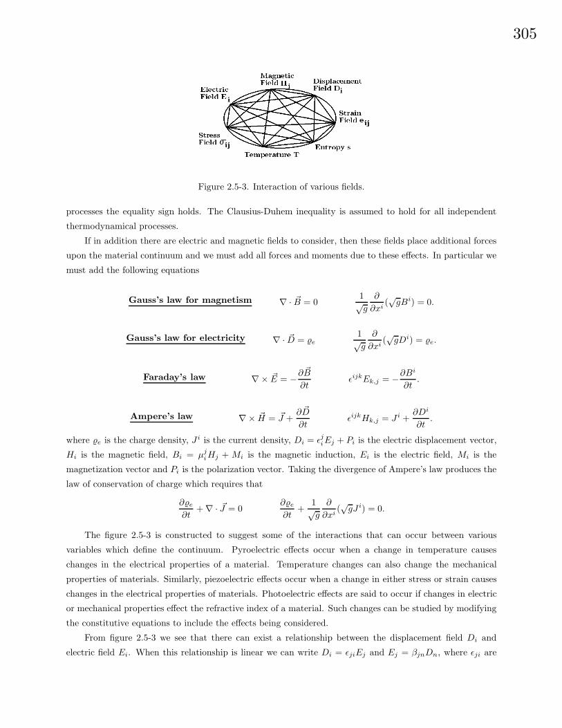
Figure 2.5-3. Interaction of various fields.
processes the equality sign holds. The Clausius-Duhem inequality is assumed to hold for all independent
thermodynamical processes.
If in addition there are electric and magnetic fields to consider, then these fields place additional forces
upon the material continuum and we must add all forces and moments due to these effects. In particular we
must add the following equations
Gauss’s law for magnetism ∇ · ~B = 01√g
∂
∂xi(√gBi) = 0.
Gauss’s law for electricity ∇ · ~D = %e1√g
∂
∂xi(√gDi) = %e.
Faraday’s law ∇× ~E = −∂~B
∂tεijkEk,j = −∂B
i
∂t.
Ampere’s law ∇× ~H = ~J +∂ ~D
∂tεijkHk,j = J i +
∂Di
∂t.
where %e is the charge density, J i is the current density, Di = εjiEj + Pi is the electric displacement vector,
Hi is the magnetic field, Bi = µjiHj + Mi is the magnetic induction, Ei is the electric field, Mi is the
magnetization vector and Pi is the polarization vector. Taking the divergence of Ampere’s law produces the
law of conservation of charge which requires that
∂%e
∂t+∇ · ~J = 0
∂%e
∂t+
1√g
∂
∂xi(√gJ i) = 0.
The figure 2.5-3 is constructed to suggest some of the interactions that can occur between various
variables which define the continuum. Pyroelectric effects occur when a change in temperature causes
changes in the electrical properties of a material. Temperature changes can also change the mechanical
properties of materials. Similarly, piezoelectric effects occur when a change in either stress or strain causes
changes in the electrical properties of materials. Photoelectric effects are said to occur if changes in electric
or mechanical properties effect the refractive index of a material. Such changes can be studied by modifying
the constitutive equations to include the effects being considered.
From figure 2.5-3 we see that there can exist a relationship between the displacement field Di and
electric field Ei. When this relationship is linear we can write Di = εjiEj and Ej = βjnDn, where εji are
306
dielectric constants and βjn are dielectric impermabilities. Similarly, when linear piezoelectric effects exist
we can write linear relations between stress and electric fields such as σij = −gkijEk and Ei = −eijkσjk,
where gkij and eijk are called piezoelectric constants. If there is a linear relation between strain and an
electric fields, this is another type of piezoelectric effect whereby eij = dijkEk and Ek = −hijkejk, where
dijk and hijk are another set of piezoelectric constants. Similarly, entropy changes can cause pyroelectric
effects. Piezooptical effects (photoelasticity) occurs when mechanical stresses change the optical properties of
the material. Electrical and heat effects can also change the optical properties of materials. Piezoresistivity
occurs when mechanical stresses change the electric resistivity of materials. Electric field changes can cause
variations in temperature, another pyroelectric effect. When temperature effects the entropy of a material
this is known as a heat capacity effect. When stresses effect the entropy in a material this is called a
piezocaloric effect. Some examples of the representation of these additional effects are as follows. The
piezoelectric effects are represented by equations of the form
σij = −hmijDm Di = dijkσjk eij = gkijDk Di = eijkejk
where hmij , dijk, gkij and eijk are piezoelectric constants.
Knowledge of the material or electric interaction can be used to help modify the constitutive equations.
For example, the constitutive equations can be modified to included temperature effects by expressing the
constitutive equations in the form
σij = cijklekl − βij∆T and eij = sijklσkl + αij∆T
where for isotropic materials the coefficients αij and βij are constants. As another example, if the strain is
modified by both temperature and an electric field, then the constitutive equations would take on the form
eij = sijklσkl + αij∆T + dmijEm.
Note that these additional effects are additive under conditions of small changes. That is, we may use the
principal of superposition to calculate these additive effects.
If the electric field and electric displacement are replaced by a magnetic field and magnetic flux, then
piezomagnetic relations can be found to exist between the variables involved. One should consult a handbook
to determine the order of magnitude of the various piezoelectric and piezomagnetic effects. For a large
majority of materials these effects are small and can be neglected when the field strengths are weak.
The Boltzmann Transport Equation
The modeling of the transport of particle beams through matter, such as the motion of energetic protons
or neutrons through bulk material, can be approached using ideas from the classical kinetic theory of gases.
Kinetic theory is widely used to explain phenomena in such areas as: statistical mechanics, fluids, plasma
physics, biological response to high-energy radiation, high-energy ion transport and various types of radiation
shielding. The problem is basically one of describing the behavior of a system of interacting particles and their
distribution in space, time and energy. The average particle behavior can be described by the Boltzmann
equation which is essentially a continuity equation in a six-dimensional phase space (x, y, z, Vx, Vy , Vz). We
307
will be interested in examining how the particles in a volume element of phase space change with time. We
introduce the following notation:
(i) ~r the position vector of a typical particle of phase space and dτ = dxdydz the corresponding spatial
volume element at this position.
(ii) ~V the velocity vector associated with a typical particle of phase space and dτv = dVxdVydVz the
corresponding velocity volume element.
(iii) ~Ω a unit vector in the direction of the velocity ~V = v~Ω.
(iv) E = 12mv
2 kinetic energy of particle.
(v) d~Ω is a solid angle about the direction ~Ω and dτ dE d~Ω is a volume element of phase space involving the
solid angle about the direction Ω.
(vi) n = n(~r, E, ~Ω, t) the number of particles in phase space per unit volume at position ~r per unit velocity
at position ~V per unit energy in the solid angle d~Ω at time t and N = N(~r, E, ~Ω, t) = vn(~r, E, ~Ω, t)
the number of particles per unit volume per unit energy in the solid angle d~Ω at time t. The quantity
N(~r, E, ~Ω, t)dτ dE d~Ω represents the number of particles in a volume element around the position ~r with
energy between E and E + dE having direction ~Ω in the solid angle d~Ω at time t.
(vii) φ(~r, E, ~Ω, t) = vN(~r, E, ~Ω, t) is the particle flux (number of particles/cm2 −Mev− sec).
(viii) Σ(E′ → E, ~Ω′ → ~Ω) a scattering cross-section which represents the fraction of particles with energy E′
and direction ~Ω′ that scatter into the energy range between E and E + dE having direction ~Ω in the
solid angle d~Ω per particle flux.
(ix) Σs(E,~r) fractional number of particles scattered out of volume element of phase space per unit volume
per flux.
(x) Σa(E,~r) fractional number of particles absorbed in a unit volume of phase space per unit volume per
flux.
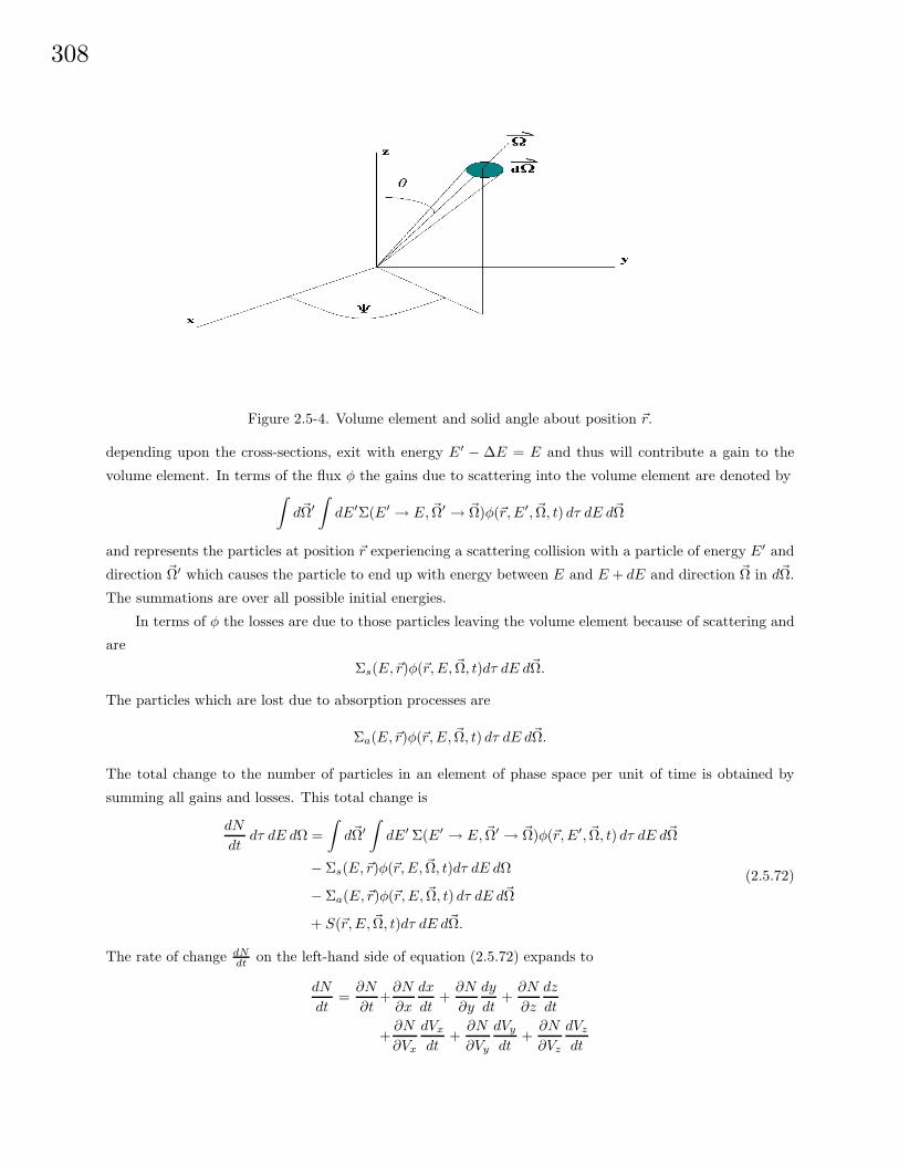
Consider a particle at time t having a position ~r in phase space as illustrated in the figure 2.5-4. This
particle has a velocity ~V in a direction ~Ω and has an energy E. In terms of dτ = dx dy dz, ~Ω and E an
element of volume of phase space can be denoted dτdEd~Ω, where d~Ω = d~Ω(θ, ψ) = sin θdθdψ is a solid angle
about the direction ~Ω.
The Boltzmann transport equation represents the rate of change of particle density in a volume element
dτ dE d~Ω of phase space and is written
d
dtN(~r, E, ~Ω, t) dτ dE d~Ω = DCN(~r, E, ~Ω, t) (2.5.71)
where DC is a collision operator representing gains and losses of particles to the volume element of phase
space due to scattering and absorption processes. The gains to the volume element are due to any sources
S(~r, E, ~Ω, t) per unit volume of phase space, with units of number of particles/sec per volume of phase space,
together with any scattering of particles into the volume element of phase space. That is particles entering
the volume element of phase space with energy E, which experience a collision, leave with some energy
E − ∆E and thus will be lost from our volume element. Particles entering with energies E′ > E may,
308
Figure 2.5-4. Volume element and solid angle about position ~r.
depending upon the cross-sections, exit with energy E′ − ∆E = E and thus will contribute a gain to the
volume element. In terms of the flux φ the gains due to scattering into the volume element are denoted by∫d~Ω′
∫dE′Σ(E′ → E, ~Ω′ → ~Ω)φ(~r, E′, ~Ω, t) dτ dE d~Ω
and represents the particles at position ~r experiencing a scattering collision with a particle of energy E′ and
direction ~Ω′ which causes the particle to end up with energy between E and E + dE and direction ~Ω in d~Ω.
The summations are over all possible initial energies.
In terms of φ the losses are due to those particles leaving the volume element because of scattering and
are
Σs(E,~r)φ(~r, E, ~Ω, t)dτ dE d~Ω.
The particles which are lost due to absorption processes are
Σa(E,~r)φ(~r, E, ~Ω, t) dτ dE d~Ω.
The total change to the number of particles in an element of phase space per unit of time is obtained by
summing all gains and losses. This total change is
dN
dtdτ dE dΩ =
∫d~Ω′
∫dE′Σ(E′ → E, ~Ω′ → ~Ω)φ(~r, E′, ~Ω, t) dτ dE d~Ω
− Σs(E,~r)φ(~r, E, ~Ω, t)dτ dE dΩ
− Σa(E,~r)φ(~r, E, ~Ω, t) dτ dE d~Ω
+ S(~r, E, ~Ω, t)dτ dE d~Ω.
(2.5.72)
The rate of change dNdt on the left-hand side of equation (2.5.72) expands to
dN
dt=∂N
∂t+∂N
∂x
dx
dt+∂N
∂y
dy
dt+∂N
∂z
dz
dt
+∂N
∂Vx
dVx
dt+∂N
∂Vy
dVy
dt+∂N
∂Vz
dVz
dt
309
which can be written asdN
dt=∂N
∂t+ ~V · ∇~rN +
~F
m· ∇~V N (2.5.73)
where d~Vdt = ~F
m represents any forces acting upon the particles. The Boltzmann equation can then be
expressed as∂N
∂t+ ~V · ∇~rN +
~F
m· ∇~V N = Gains− Losses. (2.5.74)
If the right-hand side of the equation (2.5.74) is zero, the equation is known as the Liouville equation. In
the special case where the velocities are constant and do not change with time the above equation (2.5.74)
can be written in terms of the flux φ and has the form[1v
∂
∂t+ ~Ω · ∇~r + Σs(E,~r) + Σa(E,~r)
]φ(~r, E, ~Ω, t) = DCφ (2.5.75)
where
DCφ =∫d~Ω′
∫dE′Σ(E′ → E, ~Ω′ → ~Ω)φ(~r, E′, ~Ω′, t) + S(~r, E, ~Ω, t).
The above equation represents the Boltzmann transport equation in the case where all the particles are
the same. In the case of atomic collisions of particles one must take into consideration the generation of
secondary particles resulting from the collisions.
Let there be a number of particles of type j in a volume element of phase space. For example j = p
(protons) and j = n (neutrons). We consider steady state conditions and define the quantities
(i) φj(~r, E, ~Ω) as the flux of the particles of type j.
(ii) σjk(~Ω, ~Ω′, E,E′) the collision cross-section representing processes where particles of type k moving in
direction ~Ω′ with energy E′ produce a type j particle moving in the direction ~Ω with energy E.
(iii) σj(E) = Σs(E,~r) + Σa(E,~r) the cross-section for type j particles.
The steady state form of the equation (2.5.64) can then be written as
~Ω · ∇φj(~r, E, ~Ω)+σj(E)φj(~r, E, ~Ω)
=∑
k
∫σjk(~Ω, ~Ω′, E,E′)φk(~r, E′, ~Ω′)d~Ω′dE′
(2.5.76)
where the summation is over all particles k 6= j.
The Boltzmann transport equation can be represented in many different forms. These various forms
are dependent upon the assumptions made during the derivation, the type of particles, and collision cross-
sections. In general the collision cross-sections are dependent upon three components.
(1) Elastic collisions. Here the nucleus is not excited by the collision but energy is transferred by projectile
recoil.
(2) Inelastic collisions. Here some particles are raised to a higher energy state but the excitation energy is
not sufficient to produce any particle emissions due to the collision.
(3) Non-elastic collisions. Here the nucleus is left in an excited state due to the collision processes and
some of its nucleons (protons or neutrons) are ejected. The remaining nucleons interact to form a stable
structure and usually produce a distribution of low energy particles which is isotropic in character.
310
Various assumptions can be made concerning the particle flux. The resulting form of Boltzmann’s
equation must be modified to reflect these additional assumptions. As an example, we consider modifications
to Boltzmann’s equation in order to describe the motion of a massive ion moving into a region filled with a
homogeneous material. Here it is assumed that the mean-free path for nuclear collisions is large in comparison
with the mean-free path for ion interaction with electrons. In addition, the following assumptions are made
(i) All collision interactions are non-elastic.
(ii) The secondary particles produced have the same direction as the original particle. This is called the
straight-ahead approximation.
(iii) Secondary particles never have kinetic energies greater than the original projectile that produced them.
(iv) A charged particle will eventually transfer all of its kinetic energy and stop in the media. This stopping
distance is called the range of the projectile. The stopping power Sj(E) = dEdx represents the energy
loss per unit length traveled in the media and determines the range by the relation dRj
dE = 1Sj(E) or
Rj(E) =∫ E
0dE′
Sj(E′) . Using the above assumptions Wilson, et.al.1 show that the steady state linearized
Boltzmann equation for homogeneous materials takes on the form
~Ω · ∇φj(~r, E, ~Ω)− 1Aj
∂
∂E(Sj(E)φj(~r, E, ~Ω)) + σj(E)φj(~r, E, ~Ω)
=∑k 6=j
∫dE′ d~Ω′ σjk(~Ω, ~Ω′, E,E′)φk(~r, E′, ~Ω′)
(2.5.77)
where Aj is the atomic mass of the ion of type j and φj(~r, E, ~Ω) is the flux of ions of type j moving in
the direction ~Ω with energy E.
Observe that in most cases the left-hand side of the Boltzmann equation represents the time rate of
change of a distribution type function in a phase space while the right-hand side of the Boltzmann equation
represents the time rate of change of this distribution function within a volume element of phase space due
to scattering and absorption collision processes.
Boltzmann Equation for gases
Consider the Boltzmann equation in terms of a particle distribution function f(~r, ~V , t) which can be
written as (∂
∂t+ ~V · ∇~r +
~F
m· ∇~V
)f(~r, ~V , t) = DCf(~r, ~V , t) (2.5.78)
for a single species of gas particles where there is only scattering and no absorption of the particles. An
element of volume in phase space (x, y, z, Vx, Vy, Vz) can be thought of as a volume element dτ = dxdydz
for the spatial elements together with a volume element dτv = dVxdVydVz for the velocity elements. These
elements are centered at position ~r and velocity ~V at time t. In phase space a constant velocity V1 can be
thought of as a sphere since V 21 = V 2
x +V 2y + V 2
z . The phase space volume element dτdτv changes with time
since the position ~r and velocity ~V change with time. The position vector ~r changes because of velocity
1John W. Wilson, Lawrence W. Townsend, Walter Schimmerling, Govind S. Khandelwal, Ferdous Kahn,
John E. Nealy, Francis A. Cucinotta, Lisa C. Simonsen, Judy L. Shinn, and John W. Norbury, Transport
Methods and Interactions for Space Radiations, NASA Reference Publication 1257, December 1991.
311
and the velocity vector changes because of the acceleration ~Fm . Here f(~r, ~V , t)dτdτv represents the expected
number of particles in the phase space element dτdτv at time t.
Assume there are no collisions, then each of the gas particles in a volume element of phase space centered
at position ~r and velocity ~V1 move during a time interval dt to a phase space element centered at position
~r + ~V1dt and ~V1 + ~Fmdt. If there were no loss or gains of particles, then the number of particles must be
conserved and so these gas particles must move smoothly from one element of phase space to another without
any gains or losses of particles. Because of scattering collisions in dτ many of the gas particles move into or
out of the velocity range ~V1 to ~V1 + d~V1. These collision scattering processes are denoted by the collision
operator DCf(~r, ~V , t) in the Boltzmann equation.
Consider two identical gas particles which experience a binary collision. Imagine that particle 1 with
velocity ~V1 collides with particle 2 having velocity ~V2. Denote by σ(~V1 → ~V ′1 , ~V2 → ~V ′2) dτV1dτV2 the
conditional probability that particle 1 is scattered from velocity ~V1 to between ~V ′1 and ~V ′1 + d~V ′1 and the
struck particle 2 is scattered from velocity ~V2 to between ~V ′2 and ~V ′2 +d~V ′2 . We will be interested in collisions
of the type (~V ′1 , ~V′2) → (~V1, ~V2) for a fixed value of ~V1 as this would represent the number of particles scattered
into dτV1 . Also of interest are collisions of the type (~V1, ~V2) → (~V ′1 , ~V ′2) for a fixed value ~V1 as this represents
particles scattered out of dτV1 . Imagine a gas particle in dτ with velocity ~V ′1 subjected to a beam of particles
with velocities ~V ′2 . The incident flux on the element dτdτV ′1
is |~V ′1 − ~V ′2 |f(~r, ~V ′2 , t)dτV ′2
and hence
σ(~V1 → ~V ′1 , ~V2 → ~V ′2) dτV1dτV2dt |~V ′1 − ~V ′2 |f(~r, ~V ′2 , t) dτV ′2
(2.5.79)
represents the number of collisions, in the time interval dt, which scatter from ~V ′1 to between ~V1 and ~V1 +d~V1
as well as scattering ~V ′2 to between ~V2 and ~V2 + d~V2. Multiply equation (2.5.79) by the density of particles
in the element dτdτV ′1
and integrate over all possible initial velocities ~V ′1 ,~V ′2 and final velocities ~V2 not equal
to ~V1. This gives the number of particles in dτ which are scattered into dτV1dt as
Nsin = dτdτV1dt
∫dτV2dτV ′
2
∫dτV ′
1σ(~V ′1 → ~V1, ~V
′2 → ~V2)|~V ′1 − ~V ′2 |f(~r, ~V ′1 , t)f(~r, ~V ′2 , t). (2.5.80)
In a similar manner the number of particles in dτ which are scattered out of dτV1dt is
Nsout = dτdτV1dtf(~r, ~V1, t)∫dτV2
∫dτV ′
2
∫dτV ′
1σ(~V ′1 → ~V1, ~V
′2 → ~V2)|~V2 − ~V1|f(~r, ~V2, t). (2.5.81)
Let
W (~V ′1 → ~V1, ~V′2 → ~V2) = |~V1 − ~V2|σ(~V ′1 → ~V1, ~V
′2 → ~V2) (2.5.82)
define a symmetric scattering kernel and use the relation DCf(~r, ~V , t) = Nsin − Nsout to represent the
Boltzmann equation for gas particles in the form(∂
∂t+ ~V · ∇~r +
~F
m· ∇~V
)f(~r, ~V1, t) =∫
dτV ′1
∫dτV ′
2
∫dτV2W (~V1 → ~V ′
1 , ~V2 → ~V ′2)[f(~r, ~V ′
1 , t)f(~r, ~V ′2 , t)− f(~r, ~V1, t)f(~r, ~V2, t)
].
(2.5.83)
Take the moment of the Boltzmann equation (2.5.83) with respect to an arbitrary function φ(~V1). That
is, multiply equation (2.5.83) by φ(~V1) and then integrate over all elements of velocity space dτV1 . Define
the following averages and terminology:
312
• The particle density per unit volume
n = n(~r, t) =∫dτV f(~r, ~V , t) =
+∞∫∫∫−∞
f(~r, ~V , t)dVxdVydVz (2.5.84)
where ρ = nm is the mass density.
• The mean velocity
~V1 = ~V =1n
+∞∫∫∫−∞
~V1f(~r, ~V1, t)dV1xdV1ydV1z
For any quantity Q = Q(~V1) define the barred quantity
Q = Q(~r, t) =1
n(~r, t)
∫Q(~V )f(~r, ~V , t) dτV =
1n
+∞∫∫∫−∞
Q(~V )f(~r, ~V , t)dVxdVydVz . (2.5.85)
Further, assume that ~Fm is independent of ~V , then the moment of equation (2.5.83) produces the result
∂
∂t
(nφ)
+3∑
i=1
∂
∂xi
(nV1iφ
)− n
3∑i=1
Fi
m
∂φ
∂V1i= 0 (2.5.86)
known as the Maxwell transfer equation. The first term in equation (2.5.86) follows from the integrals∫∂f(~r, ~V1, t)
∂tφ(~V1)dτV1 =
∂
∂t
∫f(~r, ~V1, t)φ(~V1) dτV1 =
∂
∂t(nφ) (2.5.87)
where differentiation and integration have been interchanged. The second term in equation (2.5.86) follows
from the integral ∫~V1∇~rf φ(~V1)dτV1 =
∫ 3∑i=1
V1i∂f
∂xiφdτV1
=3∑
i=1
∂
∂xi
(∫V1iφf dτV1
)
=3∑
i=1
∂
∂xi
(nV1iφ
).
(2.5.88)
The third term in equation (2.5.86) is obtained from the following integral where integration by parts is
employed ∫ ~F
m∇~V1
fφ dτV1 =∫ 3∑
i=1
(Fi
m
∂f
∂V1i
)φdτV1
=
+∞∫∫∫−∞
3∑i=1
φ
(Fi
m
∂f
∂V1i
)dV1xdV1ydV1y
= −∫
∂
∂V1i
(Fi
mφ
)f dτV1
= −n ∂
∂V1i
(Fi
mφ
)= −Fi
m
∂φ
∂V1i
(2.5.89)
313
since Fi does not depend upon ~V1 and f(~r, ~V , t) equals zero for Vi equal to ±∞. The right-hand side of
equation (2.5.86) represents the integral of (DCf)φ over velocity space. This integral is zero because of
the symmetries associated with the right-hand side of equation (2.5.83). Physically, the integral of (Dcf)φ
over velocity space must be zero since collisions with only scattering terms cannot increase or decrease the
number of particles per cubic centimeter in any element of phase space.
In equation (2.5.86) we write the velocities V1i in terms of the mean velocities (u, v, w) and random
velocities (Ur, Vr,Wr) with
V11 = Ur + u, V12 = Vr + v, V13 = Wr + w (2.5.90)
or ~V1 = ~Vr + ~V with ~V1 = ~Vr + ~V = ~V since ~Vr = 0 (i.e. the average random velocity is zero.) For
future reference we write equation (2.5.86) in terms of these random velocities and the material derivative.
Substitution of the velocities from equation (2.5.90) in equation (2.5.86) gives
∂(nφ)∂t
+∂
∂x
(n(Ur + u)φ
)+
∂
∂y
(n(Vr + v)φ
)+
∂
∂z
(n(Wr + w)φ
)− n
3∑i=1
Fi
m
∂φ
∂V1i= 0 (2.5.91)
or∂(nφ)∂t
+∂
∂x
(nuφ
)+
∂
∂y
(nvφ
)+
∂
∂z
(nwφ
)+
∂
∂x
(nUrφ
)+
∂
∂y
(nVrφ
)+
∂
∂z
(nWrφ
)− n3∑
i=1
Fi
m
∂φ
∂V1i= 0.
(2.5.92)
Observe that
nuφ =
+∞∫∫∫−∞
uφf(~r, ~V , t)dVxdVydVz = nuφ (2.5.93)
and similarly nvφ = nvφ, nwφ = nwφ. This enables the equation (2.5.92) to be written in the form
n∂φ
∂t+ nu
∂φ
∂x+ nv
∂φ
∂y+ nw
∂φ
∂z
+ φ
[∂n
∂t+
∂
∂x(nu) +
∂
∂y(nv) +
∂
∂z(nw)
]+
∂
∂x
(nUrφ
)+
∂
∂y
(nVrφ
)+
∂
∂z
(nWrφ
)− n3∑
i=1
Fi
m
∂φ
∂V1i= 0.
(2.5.94)
The middle bracketed sum in equation (2.5.94) is recognized as the continuity equation when multiplied by
m and hence is zero. The moment equation (2.5.86) now has the form
nDφ
Dt+
∂
∂x
(nUrφ
)+
∂
∂y
(nVrφ
)+
∂
∂z
(nWrφ
)− n
3∑i=1
Fi
m
∂φ
∂V1i= 0. (2.5.95)
Note that from the equations (2.5.86) or (2.5.95) one can derive the basic equations of fluid flow from
continuum mechanics developed earlier. We consider the following special cases of the Maxwell transfer
equation.
314
(i) In the special case φ = m the equation (2.5.86) reduces to the continuity equation for fluids. That is,
equation (2.5.86) becomes∂
∂t(nm) +∇ · (nm~V1) = 0 (2.5.96)
which is the continuity equation∂ρ
∂t+∇ · (ρ~V ) = 0 (2.5.97)
where ρ is the mass density and ~V is the mean velocity defined earlier.
(ii) In the special case φ = m~V1 is momentum, the equation (2.5.86) reduces to the momentum equation
for fluids. To show this, we write equation (2.5.86) in terms of the dyadic ~V1~V1 in the form
∂
∂t
(nm~V1
)+∇ · (nm~V1
~V1)− n~F = 0 (2.5.98)
or∂
∂t
(ρ(~Vr + ~V )
)+∇ · (ρ(~Vr + ~V )(~Vr + ~V ))− n~F = 0. (2.5.99)
Let σ = −ρ~Vr~Vr denote a stress tensor which is due to the random motions of the gas particles and
write equation (2.5.99) in the form
ρ∂~V
∂t+ ~V
∂ρ
∂t+ ρ~V (∇ · ~V ) + ~V (∇ · (ρ~V )) −∇ ·σ − n~F = 0. (2.5.100)
The term ~V(
∂ρ∂t +∇ · (ρ~V )
)= 0 because of the continuity equation and so equation (2.5.100) reduces
to the momentum equation
ρ
(∂~V
∂t+ ~V∇ · ~V
)= n~F +∇ ·σ. (2.5.101)
For ~F = q ~E + q~V × ~B + m~b, where q is charge, ~E and ~B are electric and magnetic fields, and ~b is a
body force per unit mass, together with
σ =3∑
i=1
3∑j=1
(−pδij + τij)eiej (2.5.102)
the equation (2.5.101) becomes the momentum equation
ρD~V
Dt= ρ~b−∇p+∇ · τ + nq( ~E + ~V × ~B). (2.5.103)
In the special case were ~E and ~B vanish, the equation (2.5.103) reduces to the previous momentum
equation (2.5.25) .
(iii) In the special case φ = m2~V1 · ~V1 = m
2 (V 211 +V 2
12 +V 213) is the particle kinetic energy, the equation (2.5.86)
simplifies to the energy equation of fluid mechanics. To show this we substitute φ into equation (2.5.95)
and simplify. Note thatφ =
m
2
[(Ur + u)2 + (Vr + v)2 + (Wr + w)2
]φ =
m
2
[U2
r + V 2r +W 2
r + u2 + v2 + w2] (2.5.104)
315
since uUr = vVr = wWr = 0. Let V 2 = u2 + v2 + w2 and C2r = U2
r + V 2r + W 2
r and write equation
(2.5.104) in the form
φ =m
2
(C2
r + V 2). (2.5.105)
Also note that
nUrφ =nm
2
[Ur(Ur + u)2 + Ur(Vr + v)2 + Ur(Wr + w)2
]=nm
2
[UrC2
r
2+ uU2
r + vUrVr + wUrWr
](2.5.106)
and that
nVrφ =nm
2
[VrC2
r + uVrUr + vV 2r + wVrWr
](2.5.107)
nWrφ =nm
2
[WrC2
r + uWrUr + vWrVr + wW 2r
](2.5.108)
are similar results.
We use ∂∂V1i
(φ) = mV1i together with the previous results substituted into the equation (2.5.95), and
find that the Maxwell transport equation can be expressed in the form
ρD
Dt
(C2
r
2+V 2
2
)=− ∂
∂x
(ρ[uU2
r + vUrVr + wUrWr])
− ∂
∂y
(ρ[uVrUr + vV 2
r + wVrWr])
− ∂
∂z
(ρ[uWrUr + vWrVr + wW 2
r ])
− ∂
∂x
(ρUrC2
r
2
)− ∂
∂y
(ρVrC2
r
2
)− ∂
∂z
(ρWrC2
r
2
)+ n~F · ~V .
(2.5.109)
Compare the equation (2.5.109) with the energy equation (2.5.48)
ρDe
Dt+ ρ
D
Dt
(V 2
2
)= ∇(σ · ~V )−∇ · ~q + ρ~b · ~V (2.5.110)
where the internal heat energy has been set equal to zero. Let e = C2r
2 denote the internal energy due to
random motion of the gas particles, ~F = m~b, and let
∇ · ~q =− ∂
∂x
(ρUrC2
r
2
)− ∂
∂y
(ρVrC2
r
2
)− ∂
∂z
(ρWrC2
r
2
)
=− ∂
∂x
(k∂T
∂x
)− ∂
∂y
(k∂T
∂y
)− ∂
∂z
(k∂T
∂z
) (2.5.111)
represent the heat conduction terms due to the transport of particle energy mC2r
2 by way of the random
particle motion. The remaining terms are related to the rate of change of work and surface stresses giving
− ∂
∂x
(ρ[uU2
r + vUrVr + wUrWr])
=∂
∂x(uσxx + vσxy + wσxz)
− ∂
∂y
(ρ[uVrUr + vV 2
r + wVrWr])
=∂
∂y(uσyx + vσyy + wσyz)
− ∂
∂z
(ρ[uWrUr + vWrVr + wW 2
r ])
=∂
∂z(uσzx + vσzy + wσzz) .
(2.5.112)
316
This gives the stress relations due to random particle motion
σxx =− ρU2r
σxy =− ρUrVr
σxz =− ρUrWr
σyx =− ρVrUr
σyy =− ρV 2r
σyz =− ρVrWr
σzx =− ρWrUr
σzy =− ρWrVr
σzz =− ρW 2r .
(2.5.113)
The Boltzmann equation is a basic macroscopic model used for the study of individual particle motion
where one takes into account the distribution of particles in both space, time and energy. The Boltzmann
equation for gases assumes only binary collisions as three-body or multi-body collisions are assumed to
rarely occur. Another assumption used in the development of the Boltzmann equation is that the actual
time of collision is thought to be small in comparison with the time between collisions. The basic problem
associated with the Boltzmann equation is to find a velocity distribution, subject to either boundary and/or
initial conditions, which describes a given gas flow.
The continuum equations involve trying to obtain the macroscopic variables of density, mean velocity,
stress, temperature and pressure which occur in the basic equations of continuum mechanics considered
earlier. Note that the moments of the Boltzmann equation, derived for gases, also produced these same
continuum equations and so they are valid for gases as well as liquids.
In certain situations one can assume that the gases approximate a Maxwellian distribution
f(~r, ~V , t) ≈ n(~r, t)( m
2πkT
)3/2
exp(− m
2kT~V · ~V
)(2.5.114)
thereby enabling the calculation of the pressure tensor and temperature from statistical considerations.
In general, one can say that the Boltzmann integral-differential equation and the Maxwell transfer
equation are two important formulations in the kinetic theory of gases. The Maxwell transfer equation
depends upon some gas-particle property φ which is assumed to be a function of the gas-particle velocity.
The Boltzmann equation depends upon a gas-particle velocity distribution function f which depends upon
position ~r, velocity ~V and time t. These formulations represent two distinct and important viewpoints
considered in the kinetic theory of gases.
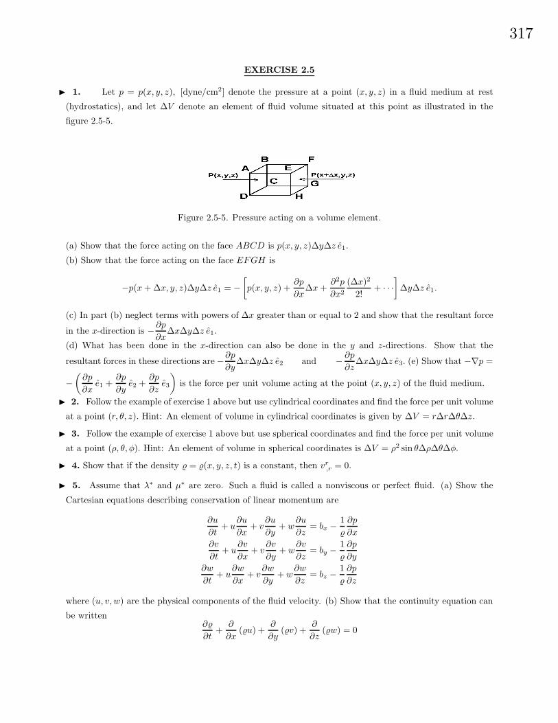
317
EXERCISE 2.5
I 1. Let p = p(x, y, z), [dyne/cm2] denote the pressure at a point (x, y, z) in a fluid medium at rest
(hydrostatics), and let ∆V denote an element of fluid volume situated at this point as illustrated in the
figure 2.5-5.
Figure 2.5-5. Pressure acting on a volume element.
(a) Show that the force acting on the face ABCD is p(x, y, z)∆y∆z e1.
(b) Show that the force acting on the face EFGH is
−p(x+ ∆x, y, z)∆y∆z e1 = −[p(x, y, z) +
∂p
∂x∆x+
∂2p
∂x2
(∆x)2
2!+ · · ·
]∆y∆z e1.
(c) In part (b) neglect terms with powers of ∆x greater than or equal to 2 and show that the resultant force
in the x-direction is − ∂p∂x
∆x∆y∆z e1.
(d) What has been done in the x-direction can also be done in the y and z-directions. Show that the
resultant forces in these directions are −∂p∂y
∆x∆y∆z e2 and − ∂p
∂z∆x∆y∆z e3. (e) Show that −∇p =
−(∂p
∂xe1 +
∂p
∂ye2 +
∂p
∂ze3
)is the force per unit volume acting at the point (x, y, z) of the fluid medium.
I 2. Follow the example of exercise 1 above but use cylindrical coordinates and find the force per unit volume
at a point (r, θ, z). Hint: An element of volume in cylindrical coordinates is given by ∆V = r∆r∆θ∆z.
I 3. Follow the example of exercise 1 above but use spherical coordinates and find the force per unit volume
at a point (ρ, θ, φ). Hint: An element of volume in spherical coordinates is ∆V = ρ2 sin θ∆ρ∆θ∆φ.
I 4. Show that if the density % = %(x, y, z, t) is a constant, then vr,r = 0.
I 5. Assume that λ∗ and µ∗ are zero. Such a fluid is called a nonviscous or perfect fluid. (a) Show the
Cartesian equations describing conservation of linear momentum are
∂u
∂t+ u
∂u
∂x+ v
∂u
∂y+ w
∂u
∂z= bx − 1
%
∂p
∂x
∂v
∂t+ u
∂v
∂x+ v
∂v
∂y+ w
∂v
∂z= by − 1
%
∂p
∂y
∂w
∂t+ u
∂w
∂x+ v
∂w
∂y+ w
∂w
∂z= bz − 1
%
∂p
∂z
where (u, v, w) are the physical components of the fluid velocity. (b) Show that the continuity equation can
be written∂%
∂t+
∂
∂x(%u) +
∂
∂y(%v) +
∂
∂z(%w) = 0
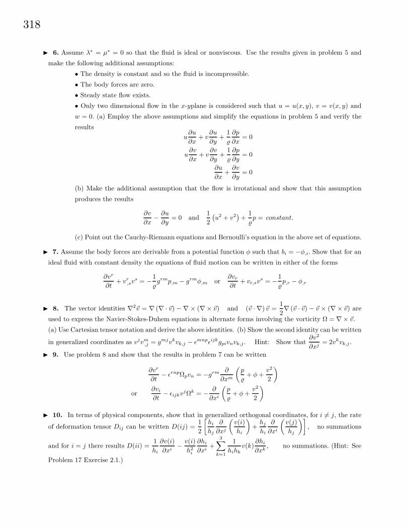
318
I 6. Assume λ∗ = µ∗ = 0 so that the fluid is ideal or nonviscous. Use the results given in problem 5 and
make the following additional assumptions:
• The density is constant and so the fluid is incompressible.
• The body forces are zero.
• Steady state flow exists.
• Only two dimensional flow in the x-yplane is considered such that u = u(x, y), v = v(x, y) and
w = 0. (a) Employ the above assumptions and simplify the equations in problem 5 and verify the
resultsu∂u
∂x+ v
∂u
∂y+
1%
∂p
∂x= 0
u∂v
∂x+ v
∂v
∂y+
1%
∂p
∂y= 0
∂u
∂x+∂v
∂y= 0
(b) Make the additional assumption that the flow is irrotational and show that this assumption
produces the results
∂v
∂x− ∂u
∂y= 0 and
12(u2 + v2
)+
1%p = constant.
(c) Point out the Cauchy-Riemann equations and Bernoulli’s equation in the above set of equations.
I 7. Assume the body forces are derivable from a potential function φ such that bi = −φ,i. Show that for an
ideal fluid with constant density the equations of fluid motion can be written in either of the forms
∂vr
∂t+ vr
,svs = −1
%grmp,m − grmφ,m or
∂vr
∂t+ vr,sv
s = −1%p,r − φ,r
I 8. The vector identities ∇2~v = ∇ (∇ · ~v) − ∇ × (∇× ~v) and (~v · ∇)~v =12∇ (~v · ~v) − ~v × (∇× ~v) are
used to express the Navier-Stokes-Duhem equations in alternate forms involving the vorticity Ω = ∇× ~v.(a) Use Cartesian tensor notation and derive the above identities. (b) Show the second identity can be written
in generalized coordinates as vjvm,j = gmjvkvk,j − εmnpεijkgpivnvk,j . Hint: Show that
∂v2
∂xj= 2vkvk,j .
I 9. Use problem 8 and show that the results in problem 7 can be written
∂vr
∂t− εrnpΩpvn = −grm ∂
∂xm
(p
%+ φ+
v2
2
)or
∂vi
∂t− εijkv
jΩk = − ∂
∂xi
(p
%+ φ+
v2
2
)
I 10. In terms of physical components, show that in generalized orthogonal coordinates, for i 6= j, the rate
of deformation tensor Dij can be written D(ij) =12
[hi
hj
∂
∂xj
(v(i)hi
)+hj
hi
∂
∂xi
(v(j)hj
)], no summations
and for i = j there results D(ii) =1hi
∂v(i)∂xi
− v(i)h2
i
∂hi
∂xi+
3∑k=1
1hihk
v(k)∂hi
∂xk, no summations. (Hint: See
Problem 17 Exercise 2.1.)
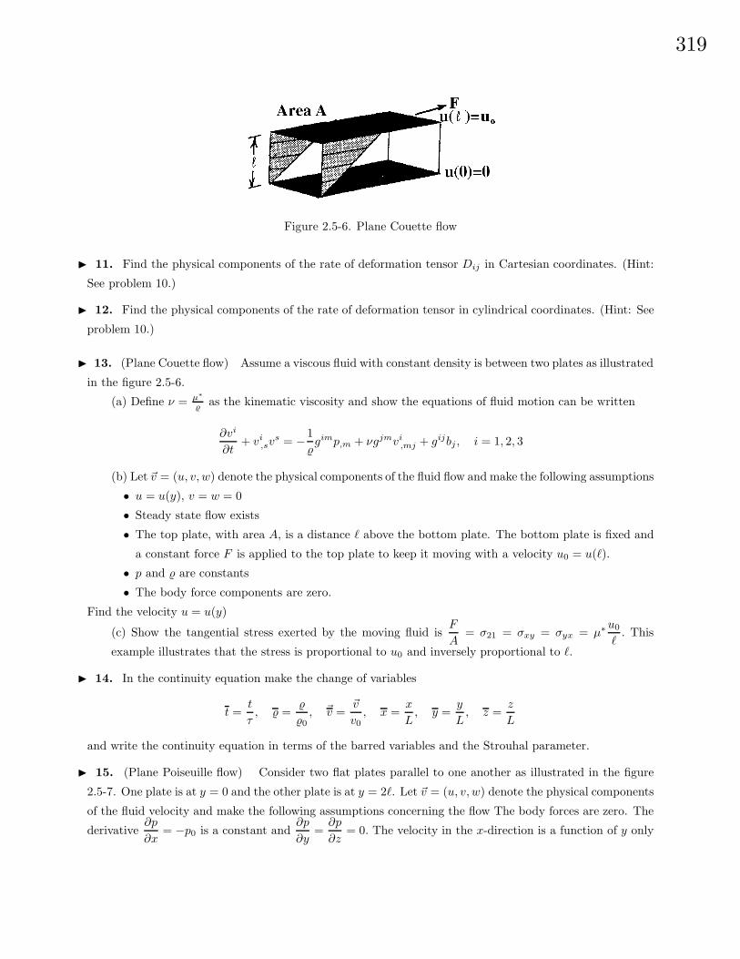
319
Figure 2.5-6. Plane Couette flow
I 11. Find the physical components of the rate of deformation tensor Dij in Cartesian coordinates. (Hint:
See problem 10.)
I 12. Find the physical components of the rate of deformation tensor in cylindrical coordinates. (Hint: See
problem 10.)
I 13. (Plane Couette flow) Assume a viscous fluid with constant density is between two plates as illustrated
in the figure 2.5-6.
(a) Define ν = µ∗
% as the kinematic viscosity and show the equations of fluid motion can be written
∂vi
∂t+ vi
,svs = −1
%gimp,m + νgjmvi
,mj + gijbj , i = 1, 2, 3
(b) Let ~v = (u, v, w) denote the physical components of the fluid flow and make the following assumptions
• u = u(y), v = w = 0
• Steady state flow exists
• The top plate, with area A, is a distance ` above the bottom plate. The bottom plate is fixed and
a constant force F is applied to the top plate to keep it moving with a velocity u0 = u(`).
• p and % are constants
• The body force components are zero.
Find the velocity u = u(y)
(c) Show the tangential stress exerted by the moving fluid isF
A= σ21 = σxy = σyx = µ∗
u0
`. This
example illustrates that the stress is proportional to u0 and inversely proportional to `.
I 14. In the continuity equation make the change of variables
t =t
τ, % =
%
%0, ~v =
~v
v0, x =
x
L, y =
y
L, z =
z
L
and write the continuity equation in terms of the barred variables and the Strouhal parameter.
I 15. (Plane Poiseuille flow) Consider two flat plates parallel to one another as illustrated in the figure
2.5-7. One plate is at y = 0 and the other plate is at y = 2`. Let ~v = (u, v, w) denote the physical components
of the fluid velocity and make the following assumptions concerning the flow The body forces are zero. The
derivative∂p
∂x= −p0 is a constant and
∂p
∂y=∂p
∂z= 0. The velocity in the x-direction is a function of y only
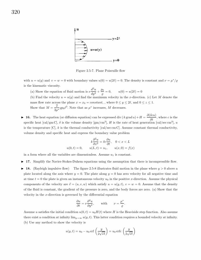
320
Figure 2.5-7. Plane Poiseuille flow
with u = u(y) and v = w = 0 with boundary values u(0) = u(2`) = 0. The density is constant and ν = µ∗/%
is the kinematic viscosity.
(a) Show the equation of fluid motion is νd2u
dy2+p0
%= 0, u(0) = u(2`) = 0
(b) Find the velocity u = u(y) and find the maximum velocity in the x-direction. (c) Let M denote the
mass flow rate across the plane x = x0 = constant, , where 0 ≤ y ≤ 2`, and 0 ≤ z ≤ 1.
Show that M =2
3µ∗%p0`
3. Note that as µ∗ increases, M decreases.
I 16. The heat equation (or diffusion equation) can be expressed div ( k gradu)+H =∂(δcu)∂t
, where c is the
specific heat [cal/gmC], δ is the volume density [gm/cm3], H is the rate of heat generation [cal/sec cm3], u
is the temperature [C], k is the thermal conductivity [cal/sec cmC]. Assume constant thermal conductivity,
volume density and specific heat and express the boundary value problem
k∂2u
∂x2= δc
∂u
∂t, 0 < x < L
u(0, t) = 0, u(L, t) = u1, u(x, 0) = f(x)
in a form where all the variables are dimensionless. Assume u1 is constant.
I 17. Simplify the Navier-Stokes-Duhem equations using the assumption that there is incompressible flow.
I 18. (Rayleigh impulsive flow) The figure 2.5-8 illustrates fluid motion in the plane where y > 0 above a
plate located along the axis where y = 0. The plate along y = 0 has zero velocity for all negative time and
at time t = 0 the plate is given an instantaneous velocity u0 in the positive x-direction. Assume the physical
components of the velocity are ~v = (u, v, w) which satisfy u = u(y, t), v = w = 0. Assume that the density
of the fluid is constant, the gradient of the pressure is zero, and the body forces are zero. (a) Show that the
velocity in the x-direction is governed by the differential equation
∂u
∂t= ν
∂2u
∂y2, with ν =
µ∗
%.
Assume u satisfies the initial condition u(0, t) = u0H(t) where H is the Heaviside step function. Also assume
there exist a condition at infinity limy→∞ u(y, t). This latter condition requires a bounded velocity at infinity.
(b) Use any method to show the velocity is
u(y, t) = u0 − u0 erf(
y
2√νt
)= u0 erfc
(y
2√νt
)
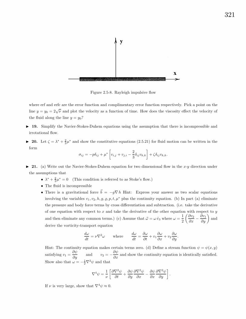
321
Figure 2.5-8. Rayleigh impulsive flow
where erf and erfc are the error function and complimentary error function respectively. Pick a point on the
line y = y0 = 2√ν and plot the velocity as a function of time. How does the viscosity effect the velocity of
the fluid along the line y = y0?
I 19. Simplify the Navier-Stokes-Duhem equations using the assumption that there is incompressible and
irrotational flow.
I 20. Let ζ = λ∗ + 23µ
∗ and show the constitutive equations (2.5.21) for fluid motion can be written in the
form
σij = −pδij + µ∗[vi,j + vj,i − 2
3δijvk,k
]+ ζδijvk,k.
I 21. (a) Write out the Navier-Stokes-Duhem equation for two dimensional flow in the x-y direction under
the assumptions that
• λ∗ + 23µ
∗ = 0 (This condition is referred to as Stoke’s flow.)
• The fluid is incompressible
• There is a gravitational force ~b = −g∇h Hint: Express your answer as two scalar equations
involving the variables v1, v2, h, g, %, p, t, µ∗ plus the continuity equation. (b) In part (a) eliminate
the pressure and body force terms by cross differentiation and subtraction. (i.e. take the derivative
of one equation with respect to x and take the derivative of the other equation with respect to y
and then eliminate any common terms.) (c) Assume that ~ω = ω e3 where ω =12
(∂v2∂x
− ∂v1∂y
)and
derive the vorticity-transport equation
dω
dt= ν∇2ω where
dω
dt=∂ω
∂t+ v1
∂ω
∂x+ v2
∂ω
∂y.
Hint: The continuity equation makes certain terms zero. (d) Define a stream function ψ = ψ(x, y)
satisfying v1 =∂ψ
∂yand v2 = −∂ψ
∂xand show the continuity equation is identically satisfied.
Show also that ω = − 12∇2ψ and that
∇4ψ =1ν
[∂∇2ψ
∂t+∂ψ
∂y
∂∇2ψ
∂x− ∂ψ
∂x
∂∇2ψ
∂y
].
If ν is very large, show that ∇4ψ ≈ 0.
322
I 22. In generalized orthogonal coordinates, show that the physical components of the rate of deformation
stress can be written, for i 6= j
σ(ij) = µ∗[hi
hj
∂
∂xj
(v(i)hi
)+hj
hi
∂
∂xi
(v(j)hj
)], no summation,
and for i 6= j 6= k
σ(ii) = −p+ 2µ∗[
1hi
∂v(i)∂xi
+1
hihjv(j)
∂hi
∂xj+
1hihk
v(k)∂hi
∂xk
]+
λ∗
h1h2h3
[∂
∂x1h2h3v(1)+
∂
∂x2h1h3v(2)+
∂
∂x3h1h2v(3)
], no summation
I 23. Find the physical components for the rate of deformation stress in Cartesian coordinates. Hint: See
problem 22.
I 24. Find the physical components for the rate of deformations stress in cylindrical coordinates. Hint: See
problem 22.
I 25. Verify the Navier-Stokes equations for an incompressible fluid can be written vi = −1%p,i +νvi,mm + bi
where ν = µ∗
% is called the kinematic viscosity.
I 26. Verify the Navier-Stokes equations for a compressible fluid with zero bulk viscosity can be written
vi = −1%p,i +
ν
3vm,mi + νvi,mm + bi with ν = µ∗
% the kinematic viscosity.
I 27. The constitutive equation for a certain non-Newtonian Stokesian fluid is σij = −pδij+βDij+γDikDkj .
Assume that β and γ are constants (a) Verify that σij,j = −p,i + βDij,j + γ(DikDkj,j +Dik,jDkj)
(b) Write out the Cauchy equations of motion in Cartesian coordinates. (See page 236).
I 28. Let the constitutive equations relating stress and strain for a solid material take into account thermal
stresses due to a temperature T . The constitutive equations have the form eij =1 + ν
Eσij− ν
Eσkk δij +αT δij
where α is a coefficient of linear expansion for the material and T is the absolute temperature. Solve for the
stress in terms of strains.
I 29. Derive equation (2.5.53) and then show that when the bulk coefficient of viscosity is zero, the Navier-
Stokes equations, in Cartesian coordinates, can be written in the conservation form
∂(%u)∂t
+∂(%u2 + p− τxx)
∂x+∂(%uv − τxy)
∂y+∂(%uw − τxz)
∂z= %bx
∂(%v)∂t
+∂(%uv − τxy)
∂x+∂(%v2 + p− τyy)
∂y+∂(%vw − τyz)
∂z= %by
∂(%w)∂t
+∂(%uw − τxz)
∂x+∂(%vw − τyz)
∂y+∂(%w2 + p− τzz)
∂z= %bz
where v1 = u,v2 = v,v3 = w and τij = µ∗(vi,j + vj,i − 23δijvk,k). Hint: Alternatively, consider 2.5.29 and use
the continuity equation.
323
I 30. Show that for a perfect gas, where λ∗ = − 23µ
∗ and η = µ∗ is a function of position, the vector form
of equation (2.5.25) is
%D~v
Dt= %~b−∇p+
43∇(η∇ · ~v) +∇(~v · ∇η) − ~v∇2η + (∇η)× (∇× ~v)− (∇ · ~v)∇η −∇× (∇× (η~v))
I 31. Derive the energy equation %D h
Dt=Dp
Dt+∂Q
∂t−∇ · ~q + Φ. Hint: Use the continuity equation.
I 32. Show that in Cartesian coordinates the Navier-Stokes equations of motion for a compressible fluid
can be written
ρDu
Dt=ρbx − ∂p
∂x+
∂
∂x
(2µ∗
∂u
∂x+ λ∗∇ · ~V
)+
∂
∂y
(µ∗(
∂u
∂y+∂v
∂x))
+∂
∂z
(µ∗(
∂w
∂x+∂u
∂z))
ρDv
Dt=ρby − ∂p
∂y+
∂
∂y
(2µ∗
∂v
∂y+ λ∗∇ · ~V
)+
∂
∂z
(µ∗(
∂v
∂z+∂w
∂y))
+∂
∂x
(µ∗(
∂w
∂y+∂w
∂x))
ρDv
Dt=ρbz − ∂p
∂z+
∂
∂z
(2µ∗
∂w
∂z+ λ∗∇ · ~V
)+
∂
∂x
(µ∗(
∂w
∂x+∂u
∂z))
+∂
∂y
(µ∗(
∂v
∂z+∂w
∂y))
where (Vx, Vy, Vz) = (u, v, w).
I 33. Show that in cylindrical coordinates the Navier-Stokes equations of motion for a compressible fluid
can be written
%
(DVr
Dt− V 2
θ
r
)=%br − ∂p
∂r+
∂
∂r
(2µ∗
∂Vr
∂r+ λ∗∇ · ~V
)+
1r
∂
∂θ
(µ∗(
1r
∂Vr
∂θ+∂Vθ
∂r− Vθ
r))
+∂
∂z
(µ∗(
∂Vr
∂z+∂Vz
∂r))
+2µ∗
r(∂Vr
∂r− 1r
∂Vθ
∂θ− Vr
r)
%
(DVθ
Dt+VrVθ
r
)=%bθ − 1
r
∂p
∂θ+
1r
∂
∂θ
(2µ∗(
1r
∂Vθ
∂θ+Vr
r) + λ∗∇ · ~V
)+
∂
∂z
(µ∗(
1r
∂Vz
∂θ+∂Vθ
∂z))
+∂
∂r
(µ∗(
1r
∂Vr
∂θ+∂Vθ
∂r− Vθ
r))
+2µ∗
r(1r
∂Vr
∂θ+∂Vθ
∂r− Vθ
r)
%DVz
Dt=%bz − ∂p
∂z+
∂
∂z
(2µ∗
∂Vz
∂z+ λ∗∇ · ~V
)+
1r
∂
∂r
(µ∗r(
∂Vr
∂z+∂Vz
∂r))
+1r
∂
∂θ
(µ∗(
1r
∂Vz
∂θ+∂Vθ
∂z))
I 34. Show that the dissipation function Φ can be written as Φ = 2µ∗DijDij + λ∗Θ2.
I 35. Verify the identities:
(a) %D
Dt(et/%) =
∂et
∂t+∇ · (et
~V ) (b) %D
Dt(et/%) = %
De
Dt+ %
D
Dt
(V 2/2
).
I 36. Show that the conservation law for heat flow is given by
∂T
∂t+∇ · (T~v − κ∇T ) = SQ
where κ is the thermal conductivity of the material, T is the temperature, ~Jadvection = T~v,~Jconduction = −κ∇T and SQ is a source term. Note that in a solid material there is no flow and so ~v = 0 and
324
the above equation reduces to the heat equation. Assign units of measurements to each term in the above
equation and make sure the equation is dimensionally homogeneous.
I 37. Show that in spherical coordinates the Navier-Stokes equations of motion for a compressible fluid can
be written
%(DVρ
Dt−V
2θ + V 2
φ
ρ) = %bρ − ∂p
∂ρ+
∂
∂ρ
(2µ∗
∂Vρ
∂ρ+ λ∗∇ · ~V
)+
1ρ
∂
∂θ
(µ∗(ρ
∂
∂ρ(Vθ/ρ) +
1ρ
∂Vρ
∂θ))
+1
ρ sin θ∂
∂φ
(µ∗(
1ρ sin θ
∂Vρ
∂φ+ ρ
∂
∂ρ(Vφ/ρ))
)+µ∗
ρ(4∂Vρ
∂ρ− 2ρ
∂Vθ
∂θ− 4Vρ
ρ− 2ρ sin θ
∂Vφ
∂φ− 2Vθ cot θ
ρ+ ρ cot θ
∂
∂ρ(Vθ/ρ) +
cot θρ
∂Vρ
∂θ)
%(DVθ
Dt+VρVθ
ρ−V
2φ cot θρ
) = %bθ − 1ρ
∂p
∂θ+
1ρ
∂
∂θ
(2µ∗
ρ(∂Vθ
∂θ+ Vρ) + λ∗∇ · ~V
)+
1ρ sin θ
∂
∂φ
(µ∗(
sin θρ
∂
∂θ(Vφ/ sin θ) +
1ρ sin θ
∂Vθ
∂φ))
+∂
∂ρ
(µ∗(ρ
∂
∂ρ(Vθ/ρ) +
1ρ
∂Vρ
∂θ))
+µ∗
ρ
[2(
1ρ
∂Vθ
∂θ− 1ρ sin θ
∂Vφ
∂φ− Vθ cot θ
ρ
)cot θ + 3
(ρ∂
∂ρ(Vθ/ρ) +
1ρ
∂Vρ
∂θ
)]%
(DVφ
Dt+VφVρ
ρ+
VθVφ cot θρ
)= %bφ − 1
ρ sin θ∂p
∂φ+
∂
∂ρ
(µ∗(
1ρ sin θ
∂Vρ
∂φ+ ρ
∂
∂ρ(Vφ/ρ)
))+
1ρ sin θ
∂
∂φ
(2µ∗
ρ
(1
sin θ∂Vφ
∂φ+ Vρ + Vθ cot θ
)+ λ∗∇ · ~V
)+
1ρ
∂
∂θ
(µ∗(
sin θρ
∂
∂θ(Vφ/ sin θ) +
1ρ sin θ
∂Vθ
∂φ
))+µ∗
ρ
[3(
1ρ sin θ
∂Vρ
∂φ+ ρ
∂
∂ρ(Vφ/ρ)
)+ 2 cot θ
(sin θρ
∂
∂θ(Vφ/ sin θ) +
1ρ sin θ
∂Vθ
∂φ
)]I 38. Verify all the equations (2.5.28).
I 39. Use the conservation of energy equation (2.5.47) together with the momentum equation (2.5.25) to
derive the equation (2.5.48).
I 40. Verify the equation (2.5.55).
I 41. Consider nonviscous flow and write the 3 linear momentum equations and the continuity equation
and make the following assumptions: (i) The density % is constant. (ii) Body forces are zero. (iii) Steady
state flow only. (iv) Consider only two dimensional flow with non-zero velocity components u = u(x, y) and
v = v(x, y). Show that there results the system of equations
u∂u
∂x+ v
∂u
∂y+
1%
∂P
∂x= 0, u
∂v
∂x+ v
∂v
∂y+
1%
∂P
∂y= 0,
∂u
∂x+∂v
∂y= 0.
Recognize that the last equation in the above set as one of the Cauchy-Riemann equations that f(z) = u− ivbe an analytic function of a complex variable. Further assume that the fluid flow is irrotational so that∂v
∂x− ∂u
∂y= 0. Show that this implies that
12(u2 + v2
)+P
%= Constant. If in addition u and v are derivable
from a potential function φ(x, y), such that u = ∂φ∂x and v = ∂φ
∂y , then show that φ is a harmonic function.
By constructing the conjugate harmonic function ψ(x, y) the complex potential F (z) = φ(x, y) + iψ(x, y) is
such that F ′(z) = u(x, y)− iv(x, y) and F ′(z) gives the velocity. The family of curves φ(x, y) =constant are
called equipotential curves and the family of curves ψ(x, y) = constant are called streamlines. Show that
these families are an orthogonal family of curves.