2.4 Wölbtorsion - georgi-dd.de · bab s 2 2 a s 2 b 2 1 ... SSs ah mm 4 200 M I S a 4 M I S cm 4...

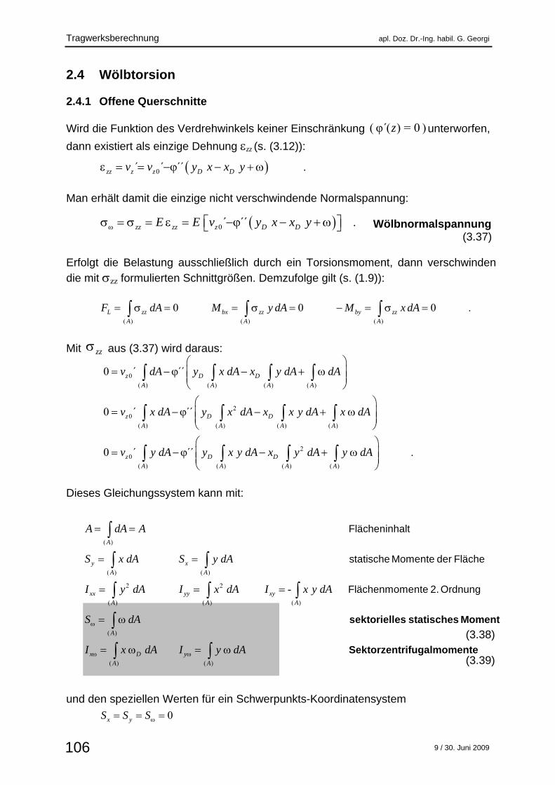
Tragwerksberechnung apl. Doz. Dr.-Ing. habil. G. Georgi

9 / 30. Juni 2009 106

2.4 Wölbtorsion 2.4.1 Offene Querschnitte Wird die Funktion des Verdrehwinkels keiner Einschränkung ( φ (́ ) = 0 )z unterworfen,

dann existiert als einzige Dehnung zz (s. (3.12)): Man erhält damit die einzige nicht verschwindende Normalspannung:

Wölbnormalspannung (3.37) Erfolgt die Belastung ausschließlich durch ein Torsionsmoment, dann verschwinden die mit zz formulierten Schnittgrößen. Demzufolge gilt (s. (1.9)):

Mit zz aus (3.37) wird daraus:

Dieses Gleichungssystem kann mit: (3.38) (3.39) und den speziellen Werten für ein Schwerpunkts-Koordinatensystem

0´ ´ ´́ . zz z z D Dv v y x x y

0´ ´́ . zz zz z D DE E v y x x y

( ) ( ) ( )

0 0 0 . L zz bx zz by zz

A A A

F dA M y dA M x dA

0

( ) ( ) ( ) ( )

20

( ) ( ) ( ) ( )

20

( ) ( ) ( ) ( )

0 ´ ´́

0 ´ ´́

0 ´ ´́ .

z D D

A A A A

z D D

A A A A

z D D

A A A A

v dA y x dA x y dA dA

v x dA y x dA x x y dA x dA

v y dA y x y dA x y dA y dA

( )

( ) ( )

2 2

( ) ( ) ( )

( )

( )

-

Flächeninhalt

statische Momente der Fläche

Flächenmomente 2. Ordnung

sektorielles statisches Moment

Sektor

A

y x

A A

xx yy xy

A A A

A

x D y

A

A dA A

S x dA S y dA

I y dA I x dA I x y dA

S dA

I x dA I y dA( ) zentrifugalmomenteA

0 x yS S S

apl. Doz. Dr.-Ing. habil. G. Georgi Tragwerksberechnung

9 / 30. Juni 2009 107

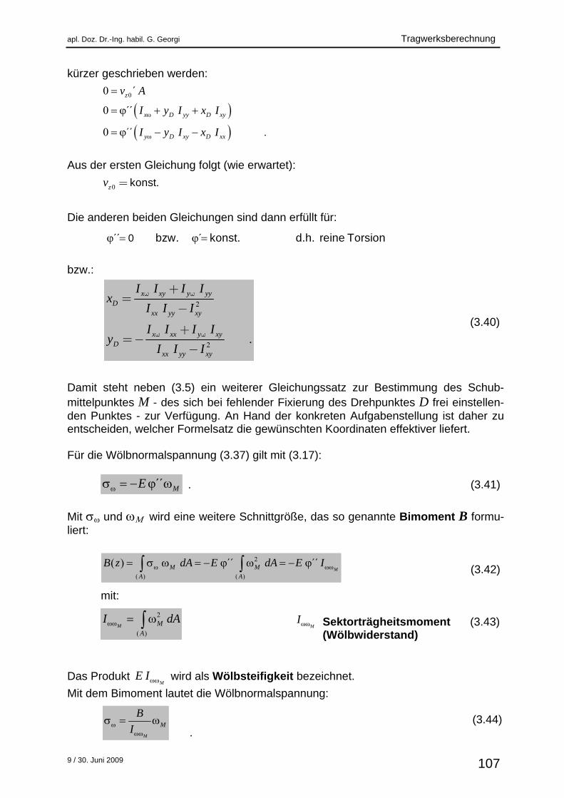
kürzer geschrieben werden: Aus der ersten Gleichung folgt (wie erwartet): Die anderen beiden Gleichungen sind dann erfüllt für: bzw.: (3.40) Damit steht neben (3.5) ein weiterer Gleichungssatz zur Bestimmung des Schub-mittelpunktes M - des sich bei fehlender Fixierung des Drehpunktes D frei einstellen-den Punktes - zur Verfügung. An Hand der konkreten Aufgabenstellung ist daher zu entscheiden, welcher Formelsatz die gewünschten Koordinaten effektiver liefert. Für die Wölbnormalspannung (3.37) gilt mit (3.17):

´´ ME . (3.41)

Mit und wird eine weitere Schnittgröße, das so genannte Bimoment B formu-liert:

(3.42)

mit:

Sektorträgheitsmoment (3.43) (Wölbwiderstand)

Das Produkt

ME I wird als Wölbsteifigkeit bezeichnet.

Mit dem Bimoment lautet die Wölbnormalspannung: (3.44) .

2

( )M M

A

I dA MI

M

M

B

I

00 ´

0 ´́

0 ´́ .

z

x D yy D xy

y D xy D xx

v A

I y I x I

I y I x I

0 .konstzv =

´́ ´0 bzw. konst. d.h. reine Torsion

2

2.

x xy y yyD

xx yy xy

x xx y xyD

xx yy xy

I I I Ix

I I I

I I I Iy

I I I

w w

w w

+=

-

+=-

-

2

( ) ( )

( ) ´́ ´́ MM M

A A

B z dA E dA E I


9 / 30. Juni 2009 108

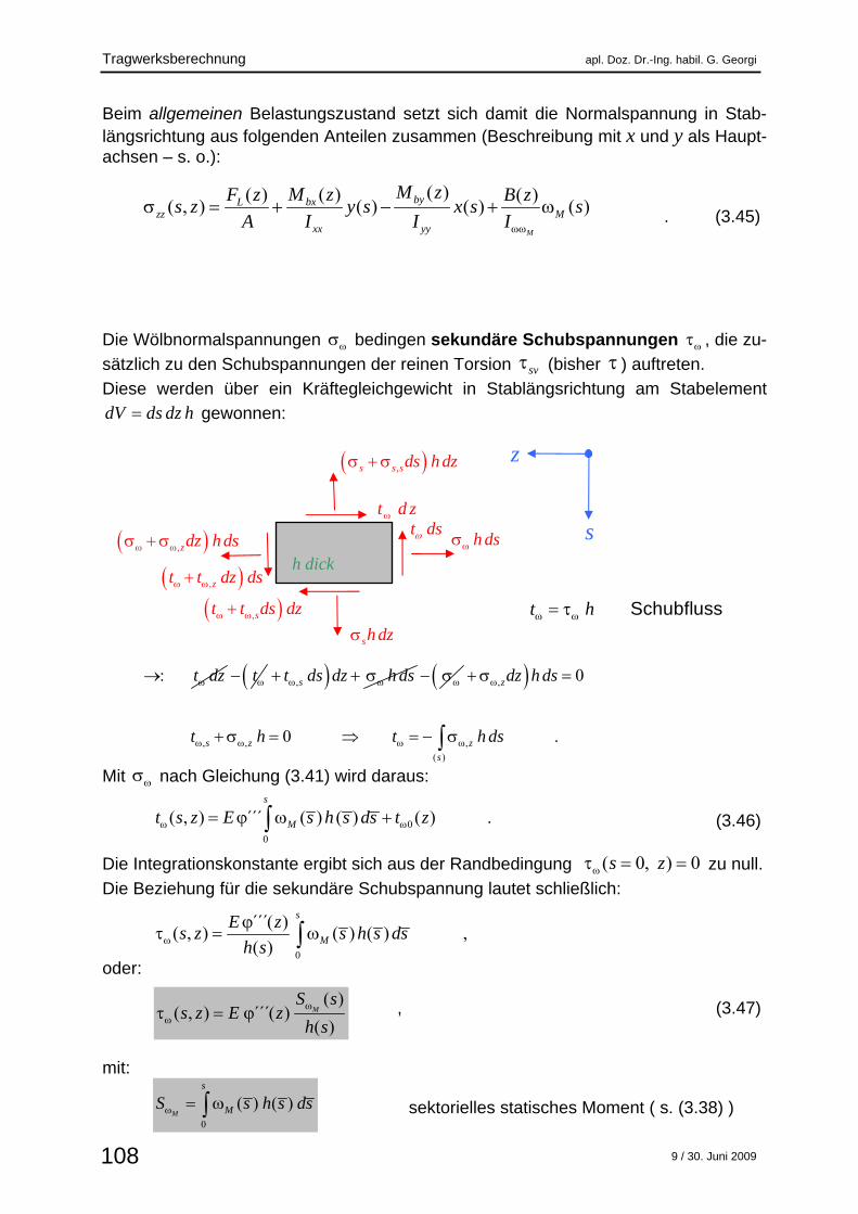
Beim allgemeinen Belastungszustand setzt sich damit die Normalspannung in Stab-längsrichtung aus folgenden Anteilen zusammen (Beschreibung mit x und y als Haupt-achsen – s. o.): . (3.45) Die Wölbnormalspannungen bedingen sekundäre Schubspannungen , die zu-

sätzlich zu den Schubspannungen der reinen Torsion sv (bisher ) auftreten.

Diese werden über ein Kräftegleichgewicht in Stablängsrichtung am Stabelement

dV ds dz h gewonnen:

Mit nach Gleichung (3.41) wird daraus:

(3.46) Die Integrationskonstante ergibt sich aus der Randbedingung ( 0, ) 0s z zu null.

Die Beziehung für die sekundäre Schubspannung lautet schließlich: oder:

, (3.47)

mit:

sektorielles statisches Moment ( s. (3.38) )

h dick

Schubflusst h

t ds

,zt t dz ds

,st t ds dz

t d z

z

s ,zdz h ds h ds

,s s sds h dz

sh dz

0

0

( , ) ´́ ´ ( ) ( ) ( ) . s

Mt s z E s h s ds t z

0

´́ (́ )( , ) ( ) ( ) ,

( )

s

M

E zs z s h s ds

h s

0

( ) ( )M

s

MS s h s ds

( )( )( ) ( )( , ) ( ) ( ) ( )

M

bybxLzz M

xx yy

M zM zF z B zs z y s x s s

A I I I

( )( , ) ´´´( )

( )

MS s

s z E zh s

: t dz t , st ds dz h ds ,

, , ,

( )

0

0 .

z

s z z

s

dz h ds

t h t h ds


9 / 30. Juni 2009 109

Das Torsionsmoment Mt wird als Summe aus dem der reinen Torsion t svM und dem

der Wölbtorsion tM aufgefasst:

(3.48) Für t svM gilt die bekannte Beziehung (3.22):

(3.22)

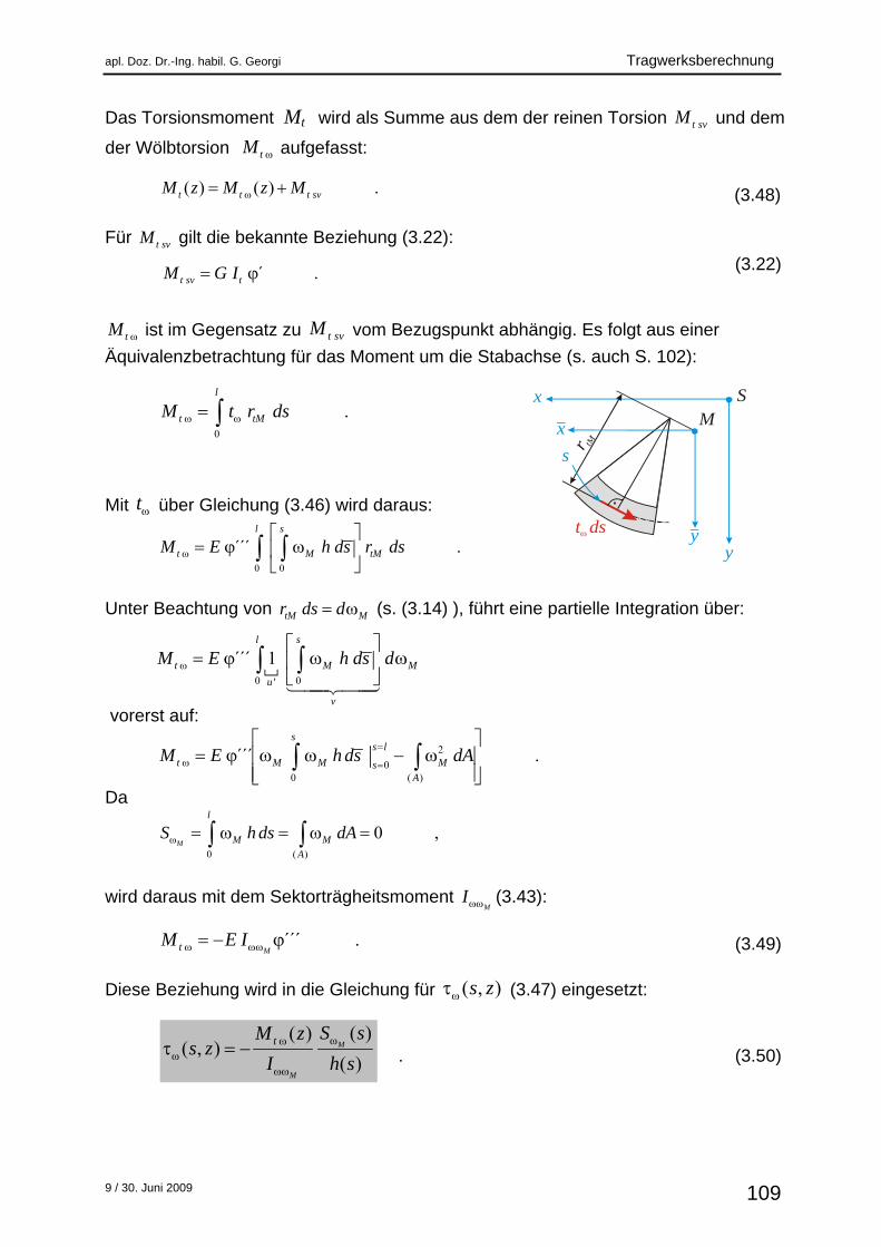
tM ist im Gegensatz zu t svM vom Bezugspunkt abhängig. Es folgt aus einer

Äquivalenzbetrachtung für das Moment um die Stabachse (s. auch S. 102):

Mit t über Gleichung (3.46) wird daraus:

0 0

´́ ´ .

l s

t M tMM E h ds r ds

Unter Beachtung von tM Mr ds d (s. (3.14) ), führt eine partielle Integration über:

vorerst auf: Da

0 ( )

0 , M

l

M M

A

S h ds dA

wird daraus mit dem Sektorträgheitsmoment

MI (3.43):

(3.49)

Diese Beziehung wird in die Gleichung für ( , )s z (3.47) eingesetzt:

. . (3.50)

x

x

yy

SM

s

t ds

r tM

´ .t sv tM G I

( ) ( ) .t t t svM z M z M

0

.l

t tMM t r ds

( )( )( , )

( )

M

M

t S sM zs z

I h s

´´´ .MtM E I

0 0'

´́ ´ 1l s

t M M

u

v

M E h ds d

2

00 ( )

´́ ´ .s

s l

t M M MsA

M E h ds dA


9 / 30. Juni 2009 110

Beim allgemeinen Belastungszustand setzt sich damit die Schubspannung tangential zur Profilmittellinie aus folgenden Anteilen zusammen (Beschreibung mit x und y als Hauptachsen – s. o.):

0 0

( )( ) ( )1( , ) ( ) ( ) ( ) ( ) .

( )

M

M

tQy Qxsz sv x y

xx yy

M zF z F zs z s S s S s S s

h s I I I (3.51)

Mit den bereitgestellten ( )t sv tM M zund(3.22) (3.49) ergibt sich nach (3.49) die

Torsions-Dgl. zu: ´´´( ) (́ ) ( )

M t tE I z G I z M z

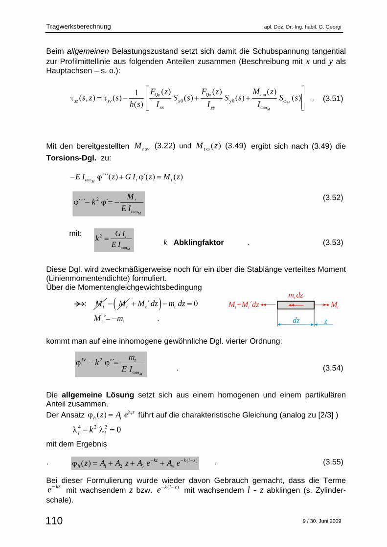
(3.52) mit: k Abklingfaktor . (3.53) Diese Dgl. wird zweckmäßigerweise noch für ein über die Stablänge verteiltes Moment (Linienmomentendichte) formuliert. Über die Momentengleichgewichtsbedingung

kommt man auf eine inhomogene gewöhnliche Dgl. vierter Ordnung: . (3.54) Die allgemeine Lösung setzt sich aus einem homogenen und einem partikulären Anteil zusammen.

Der Ansatz ( ) i zh iz A e führt auf die charakteristische Gleichung (analog zu [2/3] )

mit dem Ergebnis . . (3.55)

Bei dieser Formulierung wurde wieder davon Gebrauch gemacht, dass die Terme

kze mit wachsendem z bzw. ( )k l ze mit wachsendem l - z abklingen (s. Zylinder-

schale).

zdz

m dzt

MtM +M ´dzt t

2 ´́M

IV tmk

E I

2´́ ´ ´M

tMk

E I

2

M

tG Ik

E I

4 2 2 0i ik

( )1 2 3 4( ) kz k l z

h z A A z A e A e

: tM tM ´ 0

´ .

t t

t t

M dz m dz

M m


9 / 30. Juni 2009 111

Die Formulierung mit Hyperbelfunktionen (s. [2/3] ) führt auf: . (3.56) Die Partikulärlösung ( )p z erhält man über einen an die Funktion ( )tm z angepassten

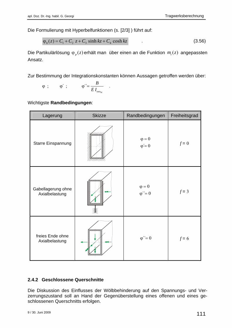
Ansatz. Zur Bestimmung der Integrationskonstanten können Aussagen getroffen werden über: Wichtigste Randbedingungen:

Lagerung Skizze Randbedingungen Freiheitsgrad

Starre Einspannung

f = 0

Gabellagerung ohne Axialbelastung

f = 3

freies Ende ohne Axialbelastung

f = 6

2.4.2 Geschlossene Querschnitte Die Diskussion des Einflusses der Wölbbehinderung auf den Spannungs- und Ver-zerrungszustand soll an Hand der Gegenüberstellung eines offenen und eines ge-schlossenen Querschnitts erfolgen.

1 2 3 4( ) sinh coshh z C C z C kz C kz

0

´ 0

0

´´ 0

´́ 0

; ´ ; ´́ .

M

B

E I


9 / 30. Juni 2009 112

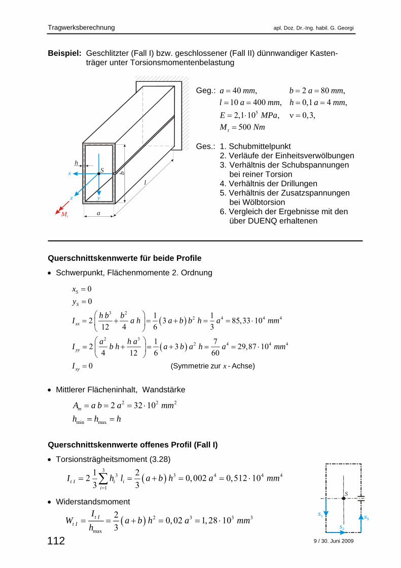
Beispiel: Geschlitzter (Fall I) bzw. geschlossener (Fall II) dünnwandiger Kasten- träger unter Torsionsmomentenbelastung Geg.: Ges.: 1. Schubmittelpunkt 2. Verläufe der Einheitsverwölbungen

3. Verhältnis der Schubspannungen bei reiner Torsion 4. Verhältnis der Drillungen 5. Verhältnis der Zusatzspannungen bei Wölbtorsion 6. Vergleich der Ergebnisse mit den über DUENQ erhaltenen

Querschnittskennwerte für beide Profile

Schwerpunkt, Flächenmomente 2. Ordnung

Mittlerer Flächeninhalt, Wandstärke

Querschnittskennwerte offenes Profil (Fall I)

Torsionsträgheitsmoment (3.28)

Widerstandsmoment

a

l

h

Mt

x

z y

S b

5

40 , 2 80 ,

10 400 , 0,1 4 ,

2,1 10 , 0,3,

500t

a mm b a mm

l a mm h a mm

E MPa

M Nm

S

s1 s3

s2

3 22 4 4 4

2 32 4 4 4

0

0

1 12 3 85,33 10

12 4 6 3

1 72 3 29,87 10

4 12 6 60

0 (Symmetrie zur - Achse)

S

S

xx

yy

xy x

x

y

h b bI a h a b b h a mm

a h aI b h a b a h a mm

I

3

3 3 4 4 4

1

1 22 0,002 0,512 10

3 3t I i ii

I h l a b h a mm

2 3 3 3

max

20,02 1, 28 10

3t I

t I

IW a b h a mm

h

2 2 2

min max

2 32 10mA a b a mm

h h h


9 / 30. Juni 2009 113

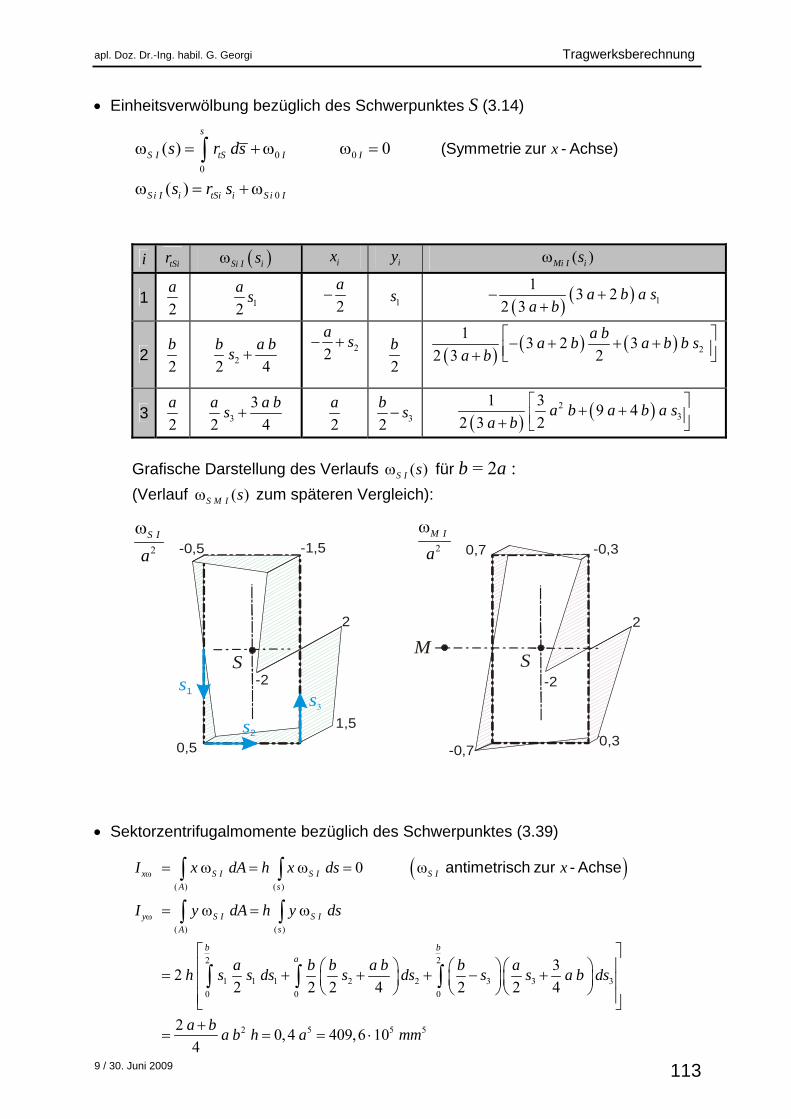
Einheitsverwölbung bezüglich des Schwerpunktes S (3.14)

i tSir Si I is ix iy ( )Mi I is

1 2

a 12

as

2

a

1s 1

13 2

2 3

a b a s

a b

2 2

b 22 4

b a b

s 22

as

2

b

2

13 2 3

2 3 2

a ba b a b b s

a b

3 2

a 3

3

2 4

a a bs

2

a 32

bs 2

3

1 39 4

2 3 2

a b a b a sa b

Grafische Darstellung des Verlaufs ( )S I s für b = 2a : (Verlauf ( )S M I s zum späteren Vergleich):

Sektorzentrifugalmomente bezüglich des Schwerpunktes (3.39)

0 0

0

0

( ) 0

( )

(Symmetrie zur - Achse)

s

S I tS I I

S i I i tSi i S i I

xs r ds

s r s

( ) ( )

( ) ( )

2 2

1 1 1 2 2 3 3 3

0 0 0

2 5 5 5

0 ω

32

2 2 2 4 2 2 4

20,4 409,6 10

4

antimetrisch zur - Achse

x S I S I S I

A s

y S I S I

A s

b ba

I x dA h x ds x

I y dA h y ds

a b b a b b ah s s ds s ds s s a b ds

a ba b h a mm

S

2 2

-2 -2

1,50,3

-1,5-0,5 -0,3

-0,7

0,7

0,5

SM

s1s3

s2

2

S I

a

2

M I

a


9 / 30. Juni 2009 114

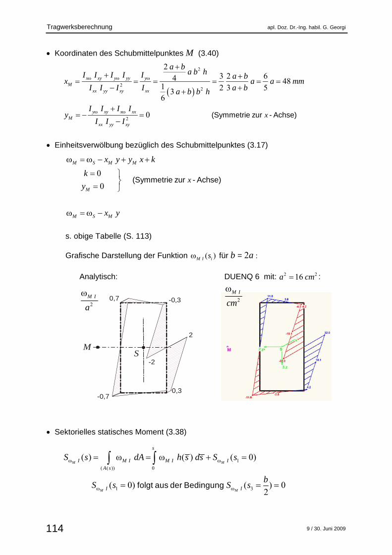
Koordinaten des Schubmittelpunktes M (3.40) Einheitsverwölbung bezüglich des Schubmittelpunktes (3.17)

s. obige Tabelle (S. 113)

Grafische Darstellung der Funktion ( )M I is für b = 2a :

Analytisch: DUENQ 6 mit: : Sektorielles statisches Moment (3.38)

0

0(Symmetrie zur - Achse)

M S M M

M

M S M

x

x y y x k

k

y

x y

2

22

2

23 2 64 48

1 2 3 536

0 (Symmetrie zur - Achse)

x xy y yy yM

xx yy xy xx

y xy x xxM

xx yy xy

x

a ba b hI I I I I a b

x a a mmI I I I a ba b b h

I I I Iy

I I I

2 216a cm

2

M I

cm

2

M I

a

2

-2

0,3

-0,3

-0,7

0,7

SM

1

( ( )) 0

1 3

( ) ω ω ( ) ( 0)

( 0) ( ) 02

folgt aus der Bedingung

M M

M M

s

I M I M I I

A s

I I

S s dA h s ds S s

bS s S s


9 / 30. Juni 2009 115

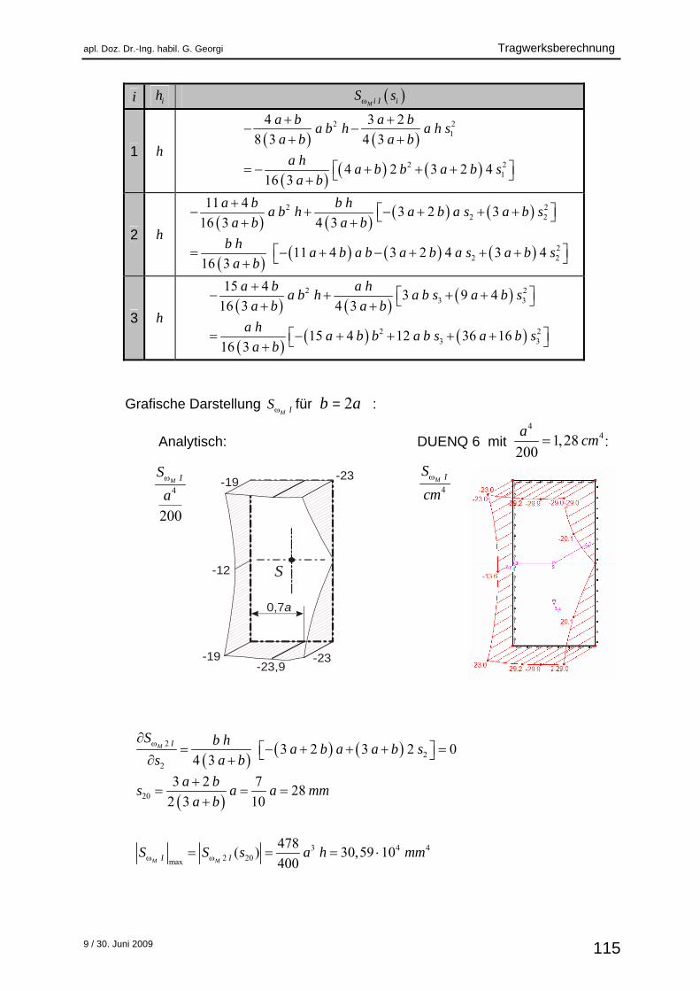
i ih M i I iS s

1 h

2 21

2 21

4 3 2

8 3 4 3

4 2 3 2 416 3

a b a ba b h a h s

a b a b

a ha b b a b s

a b

2 h

2 22 2

22 2

11 43 2 3

16 3 4 3

11 4 3 2 4 3 416 3

a b b ha b h a b a s a b s

a b a b

b ha b a b a b a s a b s

a b

3 h

2 23 3

2 23 3

15 43 9 4

16 3 4 3

15 4 12 36 1616 3

a b a ha b h a b s a b s

a b a b

a ha b b a b s a b s

a b

Grafische Darstellung M IS für b = 2a :

Analytisch: DUENQ 6 mit :

-12

-23-23,9

-23

-19

0,7a

-19

S

22

2

20

3 4 42 20max

3 2 3 2 04 3

3 2 728

2 3 10

478( ) 30,59 10

400

M

M M

I

I I

S b ha b a a b s

s a b

a bs a a mm

a b

S S s a h mm

4

200

M IS

a

4M IS

cm

441,28

200

acm


9 / 30. Juni 2009 116

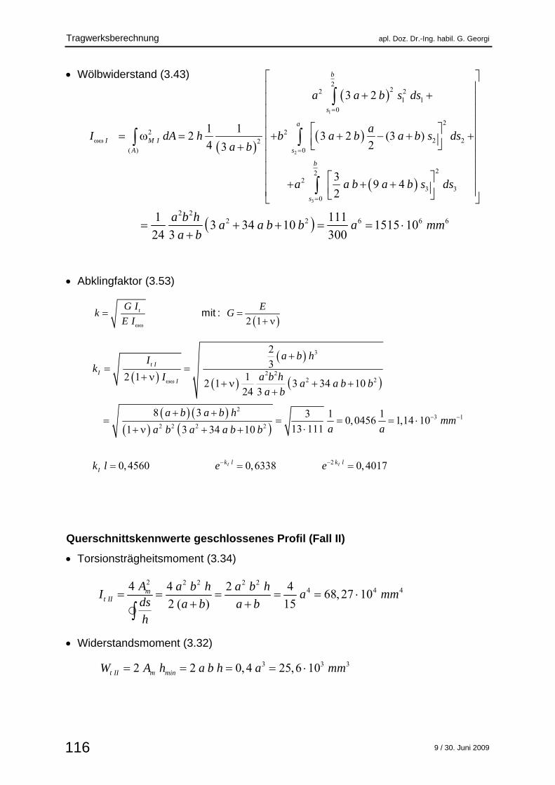
Wölbwiderstand (3.43) Abklingfaktor (3.53) Querschnittskennwerte geschlossenes Profil (Fall II)

Torsionsträgheitsmoment (3.34)

Widerstandsmoment (3.32)

1

2

3

222 2

1 1

0

22 2

2 22( ) 0

222

3 3

0

3 2

1 12 3 2 (3 )

4 23

39 4

2

b

s

a

I M I

A s

b

s

a a b s ds

aI dA h b a b a b s ds

a b

a a b a b s ds

2 2 2 2 24 4 44 4 2 4

68, 27 102 ( ) 15

mt II

A a b h a b hI a mm

ds a b a bh

3 3 32 2 0, 4 25,6 10 t II m minW A h a b h a mm

2 2

2 2 6 6 61 1113 34 10 1515 10

24 3 300

a b ha a b b a mm

a b

3

2 22 2

23 1

2 2 2 2

2

23

12 12 1 3 34 10

24 3

8 3 3 1 10,0456 1,14 10

13 1111 3 34 10

0, 4560 0,6338 0, 4017I I

t II

I

k l k lI

a b hIk

a b hIa a b b

a b

a b a b hmm

a aa b a a b b

k l e e

2 1mit :tG I E

k GE I


9 / 30. Juni 2009 117

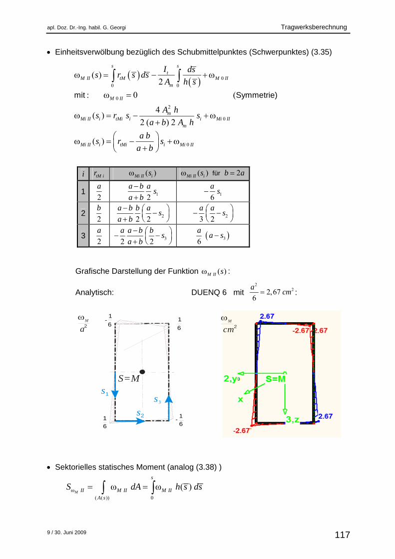
Einheitsverwölbung bezüglich des Schubmittelpunktes (Schwerpunktes) (3.35)

i tM ir ( )Mi II is ( ) 2fürMi II is b a

1 2

a 12

a b as

a b 16

a

s

2 2

b 22 2

a b b as

a b 23 2

a as

3 2

a 32 2

a a b bs

a b 36

a

a s

Grafische Darstellung der Funktion ( )M II s :

Analytisch: DUENQ 6 mit :

Sektorielles statisches Moment (analog (3.38) )

S=Ms1

s3

s2

M

a2

1-6

1-

6

1

6

1

6

M

cm2

0

0 0

0

2

0

0

( )2

: 0 (

4( )

2 ( ) 2

( )

mit Symmetrie)

s s

tM II tM M II

m

M II

mMi II i tMi i i Mi II

m

Mi II i tMi i Mi II

I dss r s ds

A h s

A hs r s s

a b A h

a bs r s

a b

222,67

6

acm

( ( )) 0

ω ω ( ) M

s

II M II M II

A s

S dA h s ds


9 / 30. Juni 2009 118

i ih M i II iS s 2für

M i II iS s b a

1 h 214

a b a hs

a b

2412120

sa

a

2 h

22

2 2

22 2

16 4

4 4

a b a b h a b b ha s s

a b a ba b b h a b

a s sa b

24

2 22

1 2 2120

s sa

a a

3 h

2

23 3

22

3 3

16 4

4 16

a b a b h a h a bb s s

a b a ba b a h b

b s sa b

24

3 32

1 2120

s sa

a a

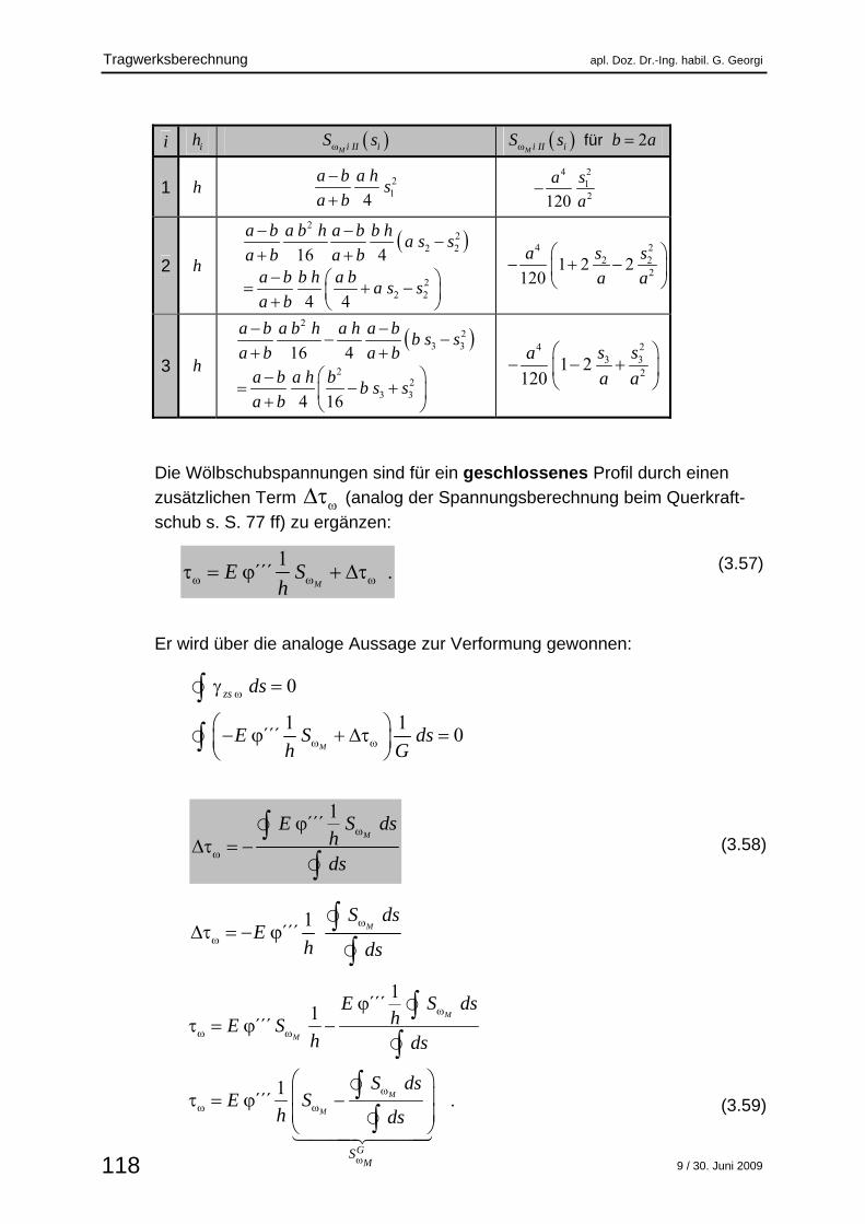
Die Wölbschubspannungen sind für ein geschlossenes Profil durch einen

zusätzlichen Term (analog der Spannungsberechnung beim Querkraft-

schub s. S. 77 ff) zu ergänzen: (3.57) Er wird über die analoge Aussage zur Verformung gewonnen:

(3.58) (3.59)

0

1 1´́ ´ 0

M

zs ds

E S dsh G

1´́ ´ .

ME S

h

1´́ ´1

´́ ´

1´́ ´ .

M

M

M

M

GM

S

E S dshE S

h ds

S dsE S

h ds

1´́ ´

ME S ds

hds

1´́ ´

MS ds

Eh ds


9 / 30. Juni 2009 119

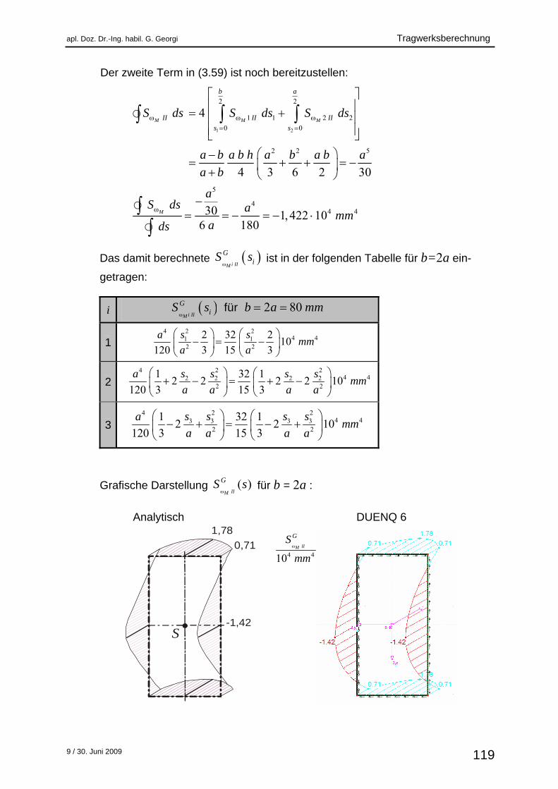
Der zweite Term in (3.59) ist noch bereitzustellen:

Das damit berechnete i IIM

GiS s

ist in der folgenden Tabelle für b=2a ein-

getragen:

i 2 80füri IIM

GiS s b a mm

1 2 24

4 41 12 2

2 32 210

120 3 15 3

s samm

a a

2 2 24

4 42 2 2 22 2

1 32 12 2 2 2 10

120 3 15 3

s s s samm

a a a a

3 2 24

4 43 3 3 32 2

1 32 12 2 10

120 3 15 3

s s s samm

a a a a

Grafische Darstellung ( )IIM

GS s

für b = 2a :

Analytisch DUENQ 6

1,78

0,71

-1,42S

1 2

2 2

1 1 2 2

0 0

2 2 5

5

44 4

4

4 3 6 2 30

30 1, 422 106 180

M M M

M

b a

II II II

s s

S ds S ds S ds

a b a b h a b a b a

a b

aS ds a

mmads

4 410IIM

GS

mm


9 / 30. Juni 2009 120

Wölbwiderstand (3.43) Abklingfaktor (s. o.) Verhältnisse der Trägheitsmomente, Widerstandsmomente, Wölbwiderstände und Abklingfaktoren

2 2

2 2 2

2 223

24 400

3 133,32 3 33

t II

t I

a b hI a b aa bI ha b ha b h

2 22 2

2 22 22 2

13 34 10

33324 33 34 10 66,6

5324

I

II

a b ha a b b

I a ba ba a b b

I a b h b a a b b aa b

22 2 62 6 6

( )

22,76 1024 180II M II

A

a b h b a aI dA mm

a b

2

23 20

23

t II

t I

W a b h a b

W a b ha b h

8880 94,2t II III

I t I II

I Ik

k I I

2 2

22 2

12

2

2

2 12 1

24

24 240 1 14,30 0,107

131

43 0 0II II

t IIII

II

k l k lII

a b hI a bk

I a b h b aa b

mma ab a

k l e e


9 / 30. Juni 2009 121

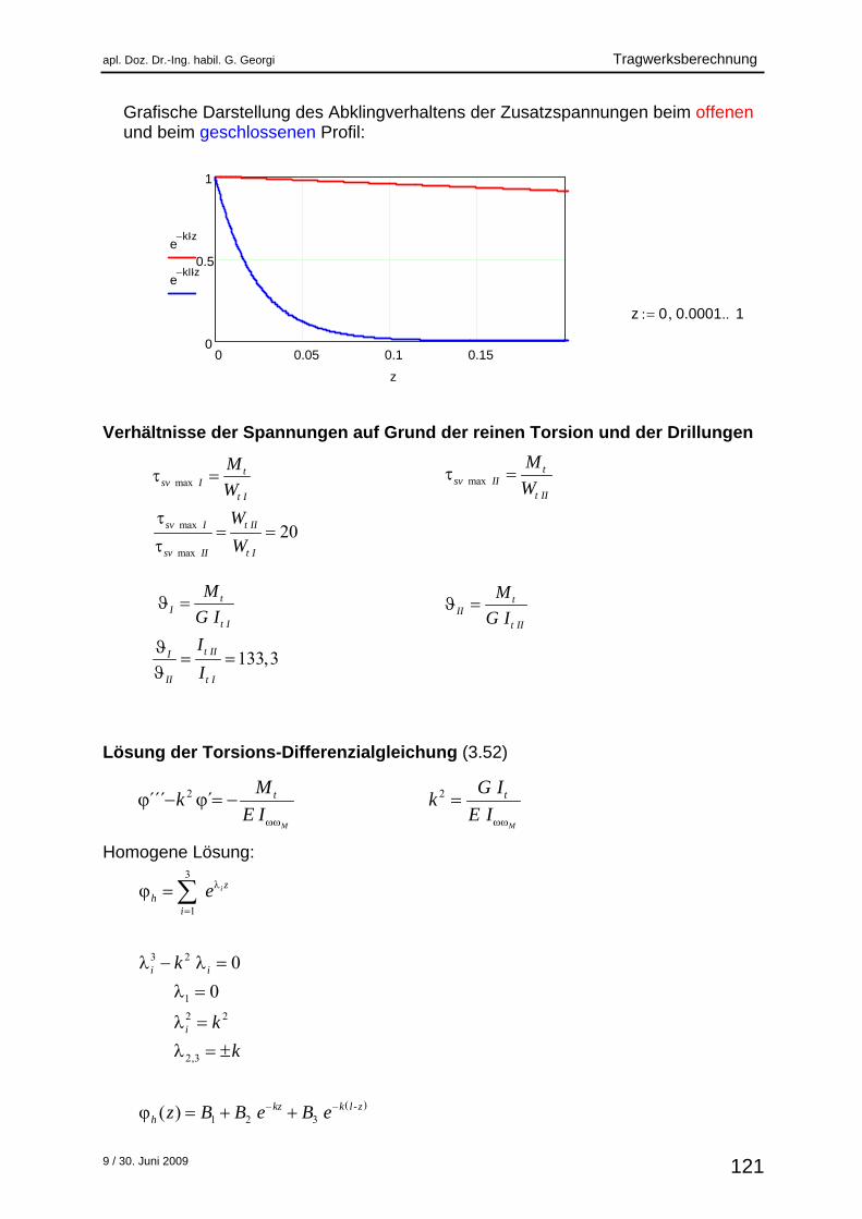
Grafische Darstellung des Abklingverhaltens der Zusatzspannungen beim offenen und beim geschlossenen Profil:

Verhältnisse der Spannungen auf Grund der reinen Torsion und der Drillungen Lösung der Torsions-Differenzialgleichung (3.52) Homogene Lösung:

maxt

sv It I

M

W

max

max

20sv I t II

sv II t I

W

W

maxt

sv IIt II

M

W

tI

t I

M

G I t

IIt II

M

G I

133,3t III

II t I

I

I

z 0 0.0001 1

2 2´´´ ´M M

t tM G Ik k

E I E I

3

1

3 2

1

2 2

2,3

1 2 3

0

0

( )

i zh

i

i i

i

kz k l-zh

e

k

k

k

z B B e B e

0 0.05 0.1 0.150

0.5

1

ekI z

ekII z

z


9 / 30. Juni 2009 122

Partikuläre Lösung: Allgemeine Lösung und deren Ableitungen: Randbedingungen, Konstanten: Spezielle Lösung: Spezielle Werte:

2

2

2

M

M

M

p

t

t

t tp

t

C z

Mk C

E I

MC

k E I

M Mz z

k E I G I

1 2 3

2 3

2 22 3

( )

(́ )

´́ ( )

kz k l-z t

t

kz k l -z t

t

kz k l-z

Mz B B e B e z

G I

Mz k B e k B e

G I

z k B e k B e

1 2 3

2 3

2 3

(0) 0 0

(́0) 0 0

´́ ( ) 0 0

kl

kl t

t

kl

B B B e

MB B e

k G I

l B e B

2

1 2

2 2

3 2

1

1

1

1

1

klt

klt

tkl

t

klt

klt

M eB

k G I e

MB

k G I e

M eB

k G I e

2 2 22

2 22

22

22

1( ) 1 1

1

1´( ) 1

1

1´´( )

1

1´´´( )

1

kl kz k l -z kltkl

t

kl kz k l-ztkl

t

kz k l -ztkl

t

kz k l-ztkl

Mz e e e k z e

k G I e

Mz e e e

G I e

M kz e e

G I e

Mz e e

E I e

2

2

2

2

1(0) 0 ( ) 1

1

1´(0) 0 ´( )

1

klt

klt

kl

tkl

t

M l el

G I kl e

eMl

G I e


9 / 30. Juni 2009 123

Verhältnisse der Zusatzspannungen auf Grund der Wölbtorsion Zusatznormalspannung (3.41)

In der Einspannung (z = 0) gilt:

Zusatzschubspannung (3.47)

In der Einspannung (z = 0) gilt:

1´´´ ( )

( ) M

E S sh s

´́ ME

2

max

2

max

max

max

2

6

20,604 7,25

16

M I

M II

I

II

a

a

Die Maxima der Beträge der Verwölbungen treten an unterschiedlichen Stellen im Querschnitt auf!

2 2

2 2

1 1 133,30,427 0,604

1 1 94, 2

I II

II I

k l k lI t II M I M I M II

k l k lII II t I M II M II M II

Ik e e

k I e e

2( ) ( ) ( )133,3

0,015( ) 8880 ( ) ( )

M M M

II II IIM M M

I I II t IIIG G G

II II t I

S s S s S sIk

k I S s S s S s

Die Maxima der Beträge der sektoriellen statischen Momente treten an unter-schiedlichen Stellen im Querschnitt auf!

2

2

2

1´´(0) ´´( ) 0

1

2´´´(0) ´´´( )

1

klt

klt

klt t

kl

M k el

G I e

M M el

E I E I e


9 / 30. Juni 2009 124

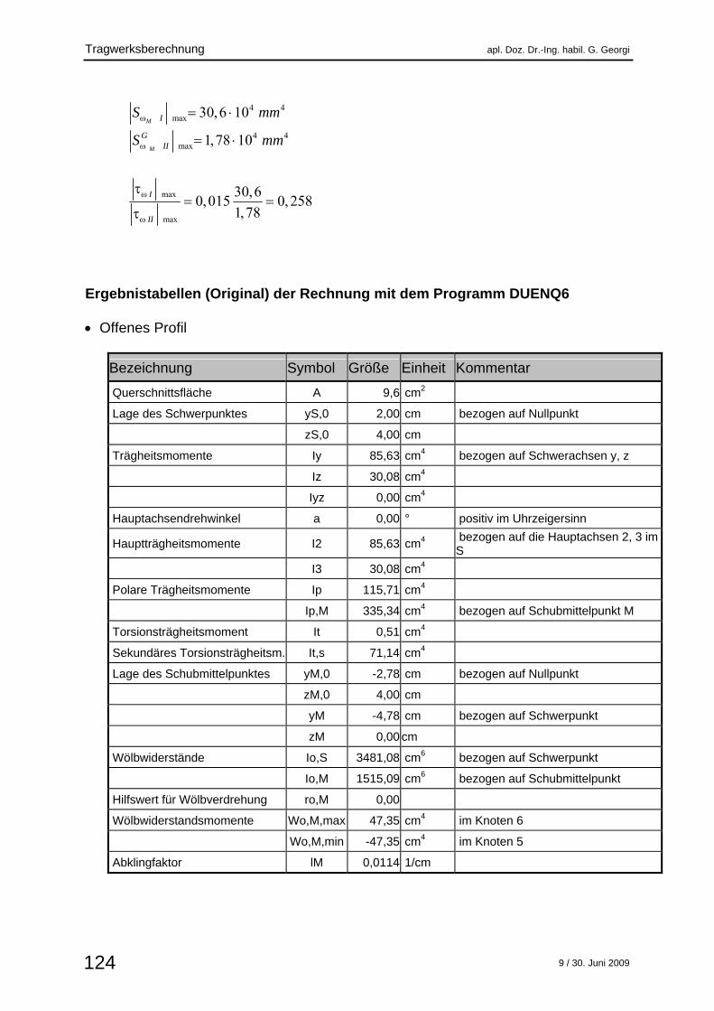
4 4max

4 4max

max

max

30,6 10

1,78 10

30,60,015 0, 258

1,78

M

M

I

GII

I

II

S mm

S mm

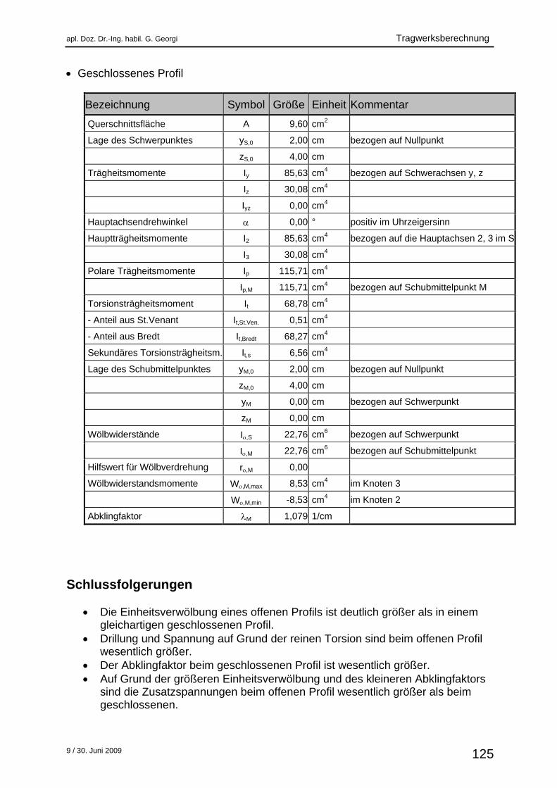
Ergebnistabellen (Original) der Rechnung mit dem Programm DUENQ6 Offenes Profil

Bezeichnung Symbol Größe Einheit Kommentar

Querschnittsfläche A 9,6 cm2

Lage des Schwerpunktes yS,0 2,00 cm bezogen auf Nullpunkt

zS,0 4,00 cm

Trägheitsmomente Iy 85,63 cm4 bezogen auf Schwerachsen y, z

Iz 30,08 cm4

Iyz 0,00 cm4

Hauptachsendrehwinkel a 0,00 ° positiv im Uhrzeigersinn

Hauptträgheitsmomente I2 85,63 cm4 bezogen auf die Hauptachsen 2, 3 im S

I3 30,08 cm4

Polare Trägheitsmomente Ip 115,71 cm4

Ip,M 335,34 cm4 bezogen auf Schubmittelpunkt M

Torsionsträgheitsmoment It 0,51 cm4

Sekundäres Torsionsträgheitsm. It,s 71,14 cm4

Lage des Schubmittelpunktes yM,0 -2,78 cm bezogen auf Nullpunkt

zM,0 4,00 cm

yM -4,78 cm bezogen auf Schwerpunkt

zM 0,00 cm

Wölbwiderstände Io,S 3481,08 cm6 bezogen auf Schwerpunkt

Io,M 1515,09 cm6 bezogen auf Schubmittelpunkt

Hilfswert für Wölbverdrehung ro,M 0,00

Wölbwiderstandsmomente Wo,M,max 47,35 cm4 im Knoten 6

Wo,M,min -47,35 cm4 im Knoten 5

Abklingfaktor lM 0,0114 1/cm


9 / 30. Juni 2009 125

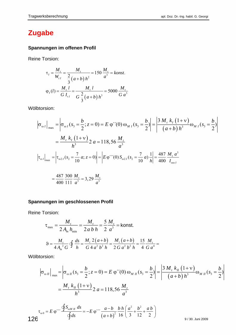
Geschlossenes Profil

Bezeichnung Symbol Größe Einheit Kommentar

Querschnittsfläche A 9,60 cm2

Lage des Schwerpunktes yS,0 2,00 cm bezogen auf Nullpunkt

zS,0 4,00 cm

Trägheitsmomente Iy 85,63 cm4 bezogen auf Schwerachsen y, z

Iz 30,08 cm4

Iyz 0,00 cm4

Hauptachsendrehwinkel 0,00 ° positiv im Uhrzeigersinn

Hauptträgheitsmomente I2 85,63 cm4 bezogen auf die Hauptachsen 2, 3 im S

I3 30,08 cm4

Polare Trägheitsmomente Ip 115,71 cm4

Ip,M 115,71 cm4 bezogen auf Schubmittelpunkt M

Torsionsträgheitsmoment It 68,78 cm4

- Anteil aus St.Venant It,St.Ven. 0,51 cm4

- Anteil aus Bredt It,Bredt 68,27 cm4

Sekundäres Torsionsträgheitsm. It,s 6,56 cm4

Lage des Schubmittelpunktes yM,0 2,00 cm bezogen auf Nullpunkt

zM,0 4,00 cm

yM 0,00 cm bezogen auf Schwerpunkt

zM 0,00 cm

Wölbwiderstände I,S 22,76 cm6 bezogen auf Schwerpunkt

I,M 22,76 cm6 bezogen auf Schubmittelpunkt

Hilfswert für Wölbverdrehung r,M 0,00

Wölbwiderstandsmomente W,M,max 8,53 cm4 im Knoten 3

W,M,min -8,53 cm4 im Knoten 2

Abklingfaktor M 1,079 1/cm

Schlussfolgerungen

Die Einheitsverwölbung eines offenen Profils ist deutlich größer als in einem gleichartigen geschlossenen Profil.

Drillung und Spannung auf Grund der reinen Torsion sind beim offenen Profil wesentlich größer.

Der Abklingfaktor beim geschlossenen Profil ist wesentlich größer. Auf Grund der größeren Einheitsverwölbung und des kleineren Abklingfaktors

sind die Zusatzspannungen beim offenen Profil wesentlich größer als beim geschlossenen.


9 / 30. Juni 2009 126

Zugabe Spannungen im offenen Profil Reine Torsion: Wölbtorsion: Spannungen im geschlossenen Profil Reine Torsion: Wölbtorsion:

32

33

150 .23

( ) 500023

t t tI

t I

t t tI

t I

M M Mkonst

W aa b h

M l M l Ml

G I G aG a b h

3

2 2 2 2max

3 3

7 7 1 487( ; 0) ´´´(0) ( )

10 10 400

487 3003, 29

400 111

tI I I

I

t t

M as a z E S s a

h I

M M

a a

3 3 33max

3 3

3 1( ; 0) ´´(0) ( ) ( )

2 2 2

12 118,56

t II I M I M I

t I t

M kb b bs z E s s

a b h

M k Ma

h a

3 3 33max

3 3

3 1( ; 0) ´´(0) ( ) ( )

2 2 2

12 118,56

t IIII II M II M II

t II t

M kb b bs z E s s

a b h

M k Ma

h a

max 3min

5.

2 2 2t t t

m

M M M

A h a b h a konst

2 2 2 2 2 4

2 15

4 4 2 4t tt t

m

M a b M a bM Mds

A G h G a b h G a b h G a

2 2

0 2´́ ´ ´́ ´16 3 12 2

M IIS ds a b b h a b a bE E

ds a b


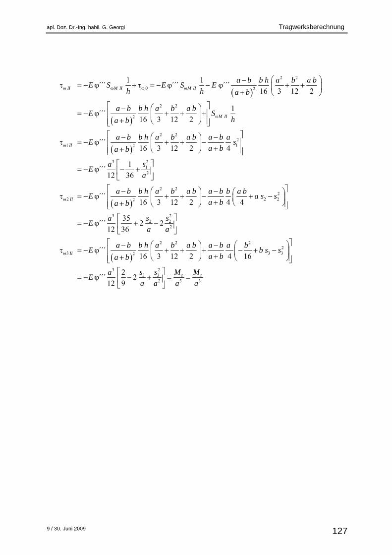
9 / 30. Juni 2009 127

2 2

0 2

2 2

2

2 22

1 12

3

1 1´́ ´ ´́ ´ ´́ ´

16 3 12 2

1´́ ´

16 3 12 2

´́ ´16 3 12 2 4

1´́ ´

12 36

II M II M II

M II

II

a b b h a b a bE S E S E

h h a b

a b b h a b a bE S

ha b

a b b h a b a b a b aE s

a ba b

aE

212

2 22

2 2 22

232 2

2

2 2 22

3 3 32

´́ ´16 3 12 2 4 4

35´́ ´ 2 2

12 36

´́ ´16 3 12 2 4 16

II

II

s

a

a b b h a b a b a b b a bE a s s

a ba b

s saE

a a

a b b h a b a b a b a bE b s s

a ba b

E

23

3 32 3 3

2´́ ´ 2

12 9t ts s M Ma

a a a a

2.4 Wölbtorsion - georgi-dd.de · bab s 2 2 a s 2 b 2 1 ... SSs ah mm 4 200 M I S a 4 M I S cm 4...

Documents

Transcript of 2.4 Wölbtorsion - georgi-dd.de · bab s 2 2 a s 2 b 2 1 ... SSs ah mm 4 200 M I S a 4 M I S cm 4...