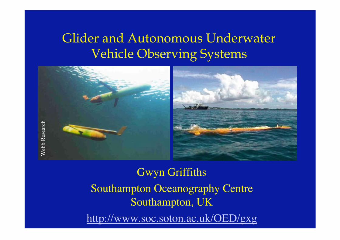
Glider and Autonomous UnderwaterVehicle Observing Systems

Gwyn GriffithsSouthampton Oceanography Centre

Southampton, UKhttp://www.soc.soton.ac.uk/OED/gxg

Webb Research

Outline of the lecture

!Glider and AUV technology - where are we?

! Sampling strategies for autonomous vehicles

! Sensors for use on AUVs

! Examples of glider & AUV applications relevant(in the broadest sense) to HAB studies

! Removing barriers to using new technologies

! Conclusions

A ‘Health Warning’ …“Several authors urge the deployment of new technologies(in the Census of Marine Life Special Issue of Oceanography) …and in all these there is in my opinion a lack of realism aboutwhat they measure”

“Maps of biological variables derived from any surveyrepresent no more than an unverifiable approximation to thetrue distribution at the central moment”

Alan Longhurst, Letter to the Editor. Oceanography, 13(2): 3-4.

“The goal of remote species identification is of immenseimportance and stirs new thinking”

Response by Jesse Ausubel, Oceanography, 13(2): 4.

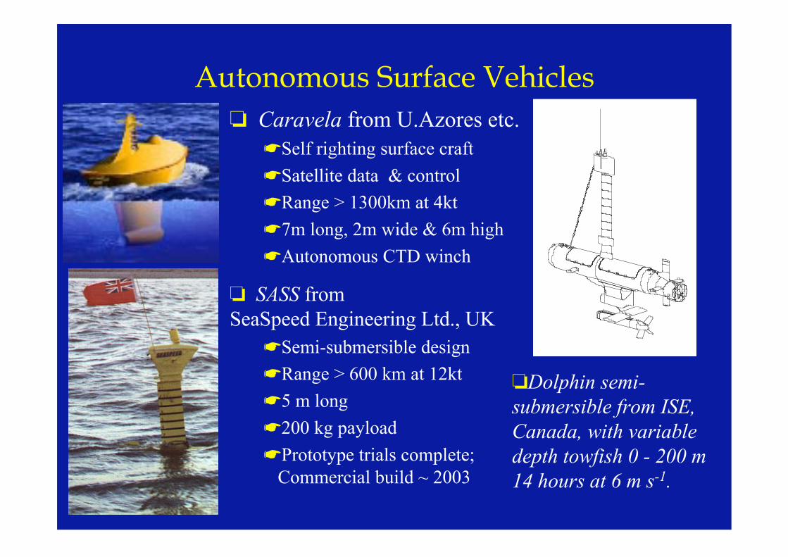
Autonomous Surface Vehicles

! SASS from SeaSpeed Engineering Ltd., UK

"Semi-submersible design

"Range > 600 km at 12kt

"5 m long

"200 kg payload

"Prototype trials complete; Commercial build ~ 2003

! Caravela from U.Azores etc."Self righting surface craft

"Satellite data & control

"Range > 1300km at 4kt

"7m long, 2m wide & 6m high

"Autonomous CTD winch

!Dolphin semi-submersible from ISE,Canada, with variabledepth towfish 0 - 200 m14 hours at 6 m s-1.

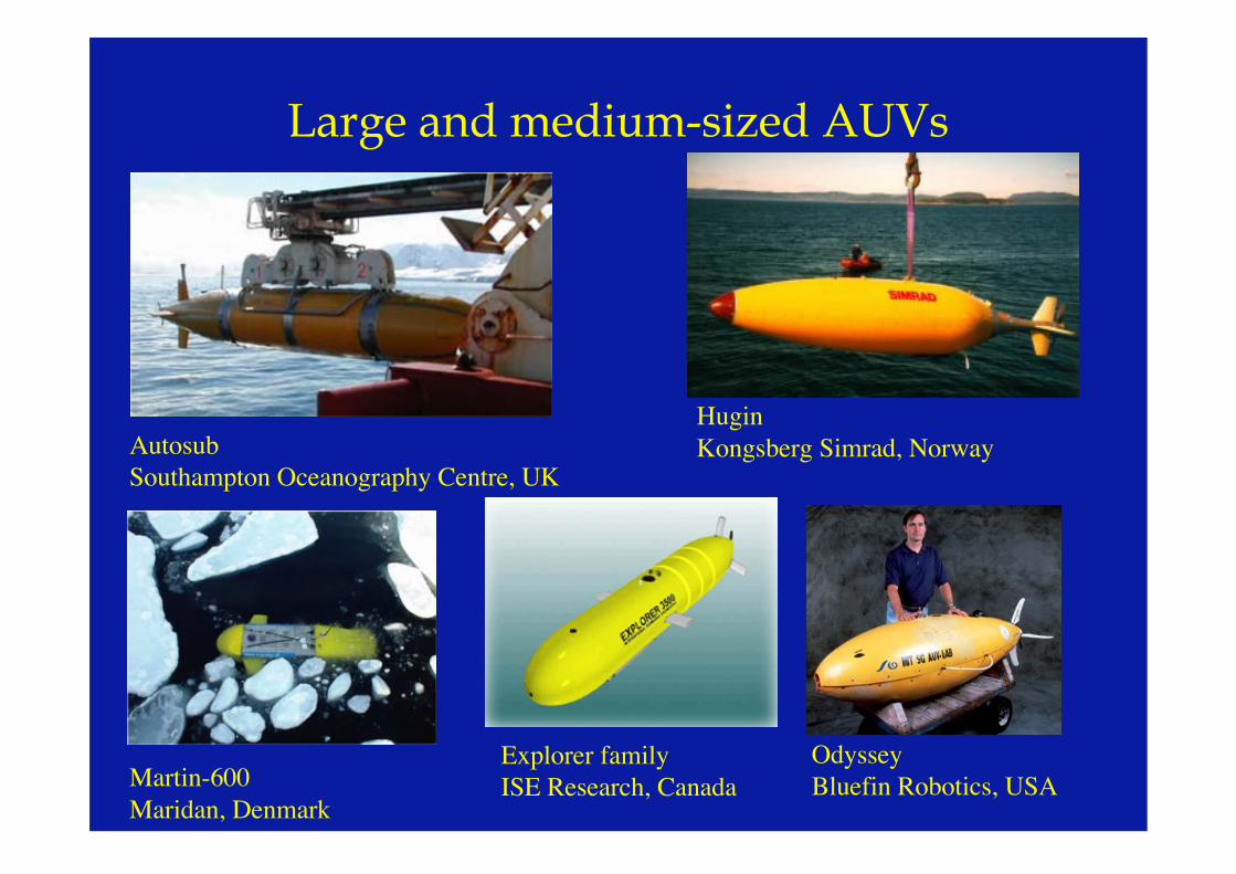
Large and medium-sized AUVs

AutosubSouthampton Oceanography Centre, UK

Martin-600Maridan, Denmark

HuginKongsberg Simrad, Norway

OdysseyBluefin Robotics, USA

Explorer familyISE Research, Canada

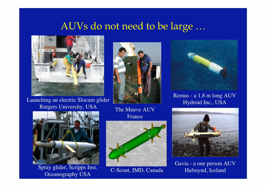
AUVs do not need to be large …

Launching an electric Slocum gliderRutgers University, USA

Spray glider, Scripps Inst.Oceanography USA

The Mauve AUVFrance

Remus - a 1.8 m long AUVHydroid Inc., USA

Gavia - a one person AUVHafmynd, IcelandC-Scout, IMD, Canada

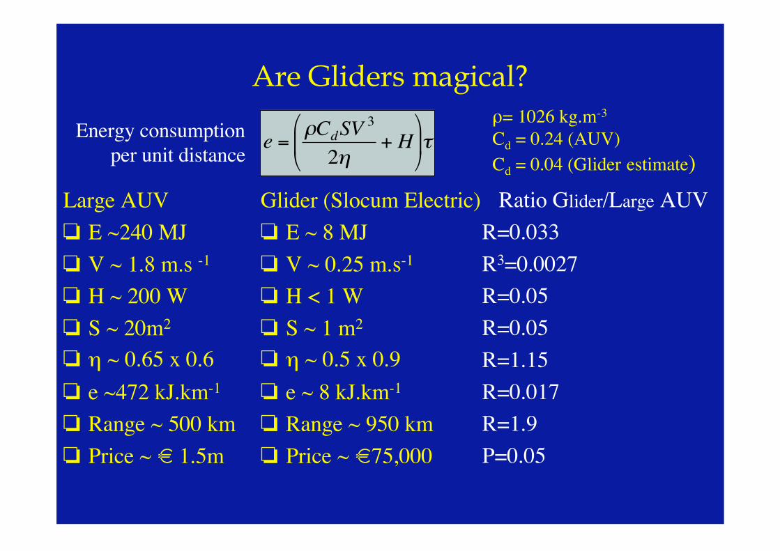
Are Gliders magical?

Large AUV! E ~240 MJ! V ~ 1.8 m.s -1

! H ~ 200 W! S ~ 20m2

! η ~ 0.65 x 0.6! e ~472 kJ.km-1

! Range ~ 500 km! Price ~ € 1.5m

Glider (Slocum Electric)! E ~ 8 MJ! V ~ 0.25 m.s-1

! H < 1 W! S ~ 1 m2

! η ~ 0.5 x 0.9! e ~ 8 kJ.km-1

! Range ~ 950 km! Price ~ €75,000

e = ρCdSV3

2η+ H

τ

Energy consumptionper unit distance

Ratio Glider/Large AUVR=0.033R3=0.0027R=0.05R=0.05R=1.15R=0.017R=1.9P=0.05

ρ= 1026 kg.m-3

Cd = 0.24 (AUV)Cd = 0.04 (Glider estimate)

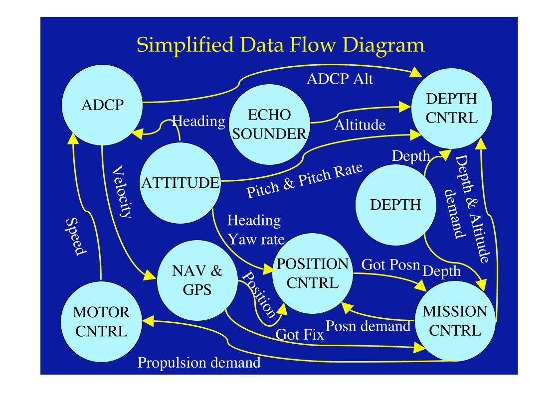
Position

Simplified Data Flow Diagram

ADCP ECHOSOUNDER

DEPTHCNTRL

ATTITUDEDEPTH

MOTORCNTRL

MISSIONCNTRL

NAV &GPS

POSITIONCNTRL

ADCP Alt

Altitude

Pitch & Pitch R

ateDepth

DepthGot Posn

Posn demand

VelocitySpeed

Heading

HeadingYaw rate

Propulsion demand

Got Fix

Depth &

Altitude

demand

Depth and Pitch Controller

Dφ

++

+ ++-

Depth

Depth demand

PzLimit pitchdemand

Pitch

Pitch rate

PφStern Planedemand

Proportional Depth controllerwith proportional & derivativepitch control

Software control

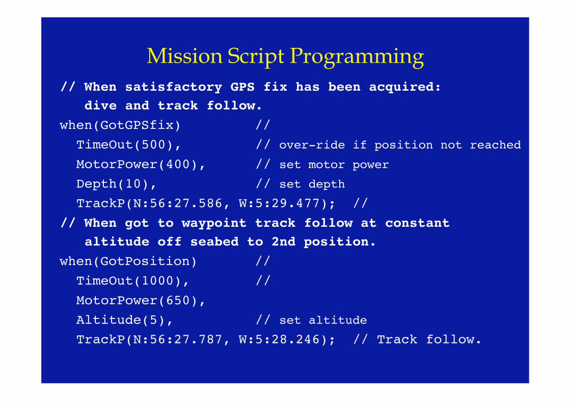
// When satisfactory GPS fix has been acquired: dive and track follow.when(GotGPSfix) // TimeOut(500), // over-ride if position not reached

MotorPower(400), // set motor power Depth(10), // set depth TrackP(N:56:27.586, W:5:29.477); //

// When got to waypoint track follow at constant altitude off seabed to 2nd position.when(GotPosition) // TimeOut(1000), //

MotorPower(650), Altitude(5), // set altitude TrackP(N:56:27.787, W:5:28.246); // Track follow.

Mission Script Programming

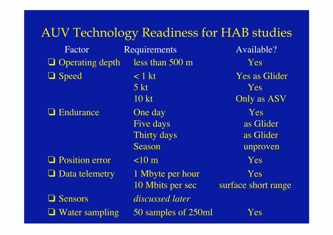
AUV Technology Readiness for HAB studies

! Operating depth less than 500 m Yes! Speed < 1 kt Yes as Glider

5 kt Yes10 kt Only as ASV

! Endurance One day Yes Five days as Glider

Thirty days as GliderSeason unproven

! Position error <10 m Yes! Data telemetry 1 Mbyte per hour Yes

10 Mbits per sec surface short range! Sensors discussed later! Water sampling 50 samples of 250ml Yes

Factor Requirements Available?

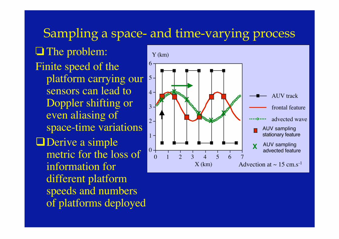
Sampling a space- and time-varying process! The problem:Finite speed of theplatform carrying oursensors can lead toDoppler shifting oreven aliasing ofspace-time variations

!Derive a simplemetric for the loss ofinformation fordifferent platformspeeds and numbersof platforms deployed

0

1

2

3

4

5

6Y (km)

0 1 2 3 4 5 6 7X (km)

advected wave

frontal feature

AUV trackXX X

XX

X

AUV samplingstationary feature

AUV samplingadvected featureX

Advection at ~ 15 cm.s-1

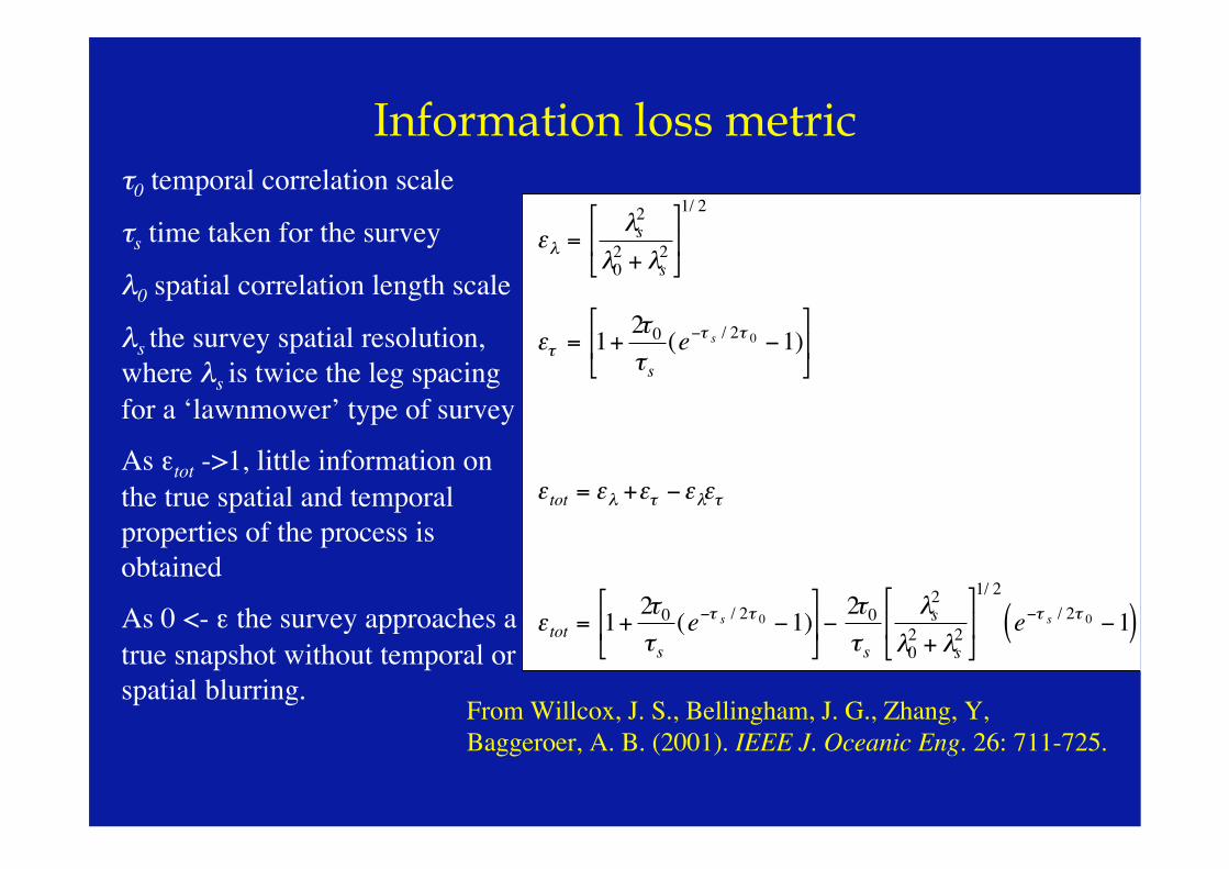
Information loss metric

ελ =λs2

λ02 + λs

2

1/ 2

ετ = 1+ 2τ0τs(e−τ s / 2τ 0 −1)

ε tot = ελ +ετ −ελετ

ε tot = 1+ 2τ0τs(e−τ s / 2τ 0 −1)

−2τ0τs

λs2

λ02 + λs

2

1/ 2

e−τ s / 2τ 0 −1( )

τ0 temporal correlation scale

τs time taken for the survey

λ0 spatial correlation length scale

λs the survey spatial resolution,where λs is twice the leg spacingfor a ‘lawnmower’ type of survey

As εtot ->1, little information onthe true spatial and temporalproperties of the process isobtained

As 0 <- ε the survey approaches atrue snapshot without temporal orspatial blurring.

From Willcox, J. S., Bellingham, J. G., Zhang, Y,Baggeroer, A. B. (2001). IEEE J. Oceanic Eng. 26: 711-725.

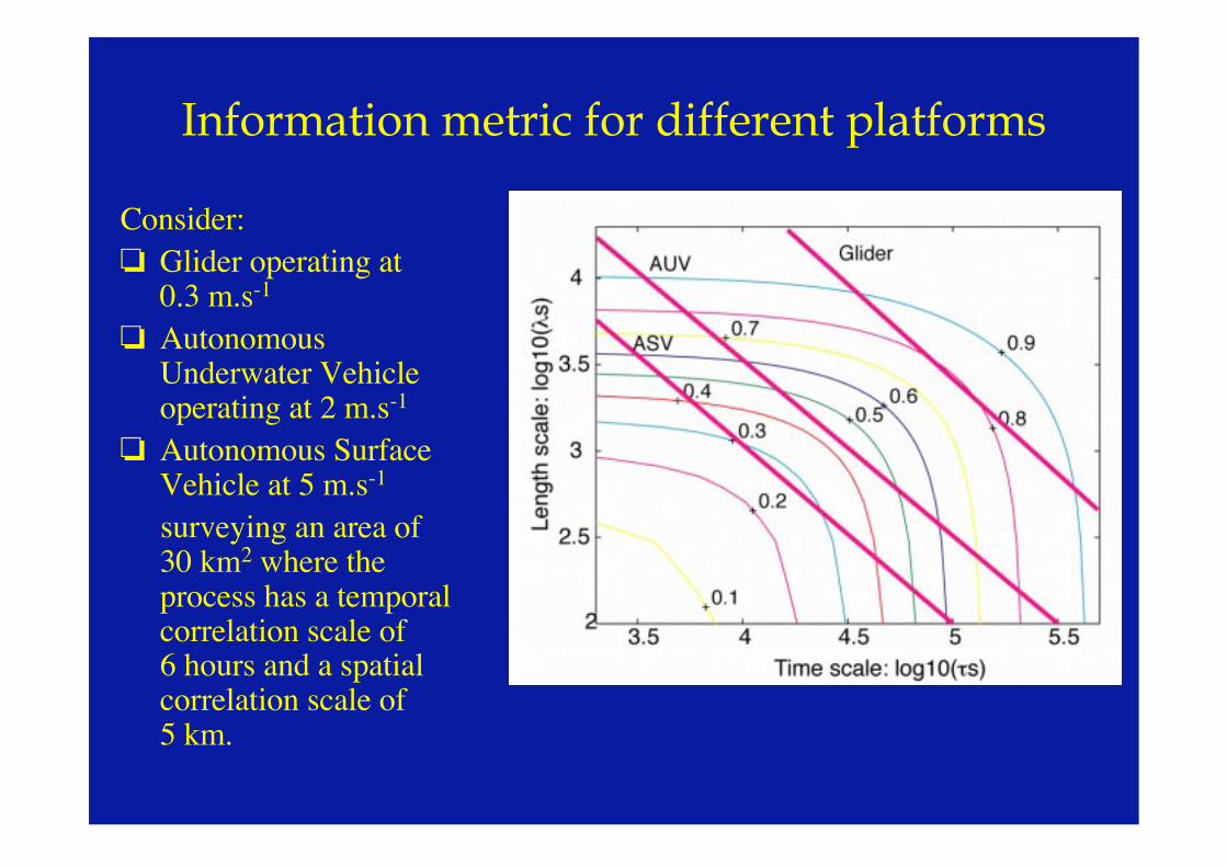
Information metric for different platforms

Consider:! Glider operating at0.3 m.s-1

! AutonomousUnderwater Vehicleoperating at 2 m.s-1

! Autonomous SurfaceVehicle at 5 m.s-1

surveying an area of30 km2 where theprocess has a temporalcorrelation scale of6 hours and a spatialcorrelation scale of5 km.

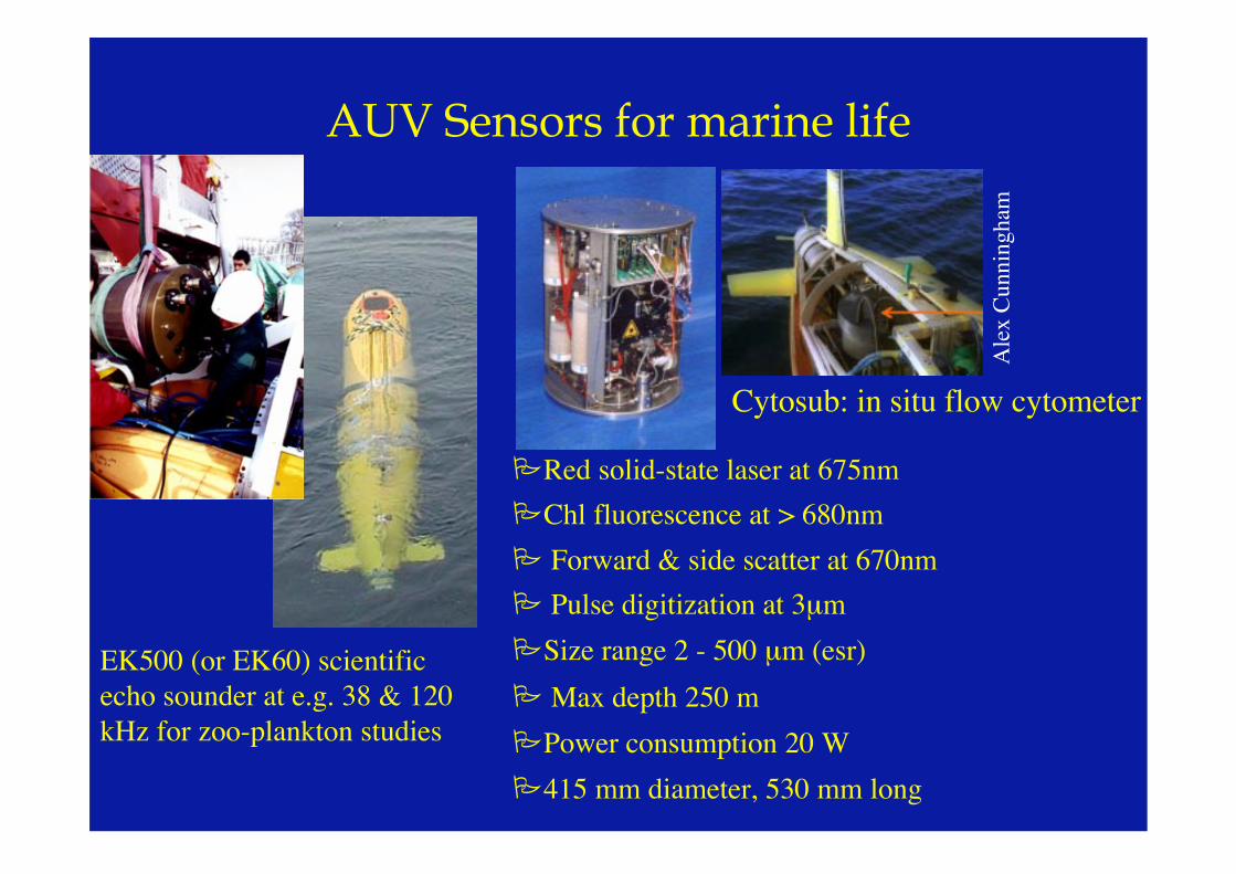
AUV Sensors for marine life

EK500 (or EK60) scientificecho sounder at e.g. 38 & 120kHz for zoo-plankton studies

!Red solid-state laser at 675nm!Chl fluorescence at > 680nm! Forward & side scatter at 670nm! Pulse digitization at 3µm!Size range 2 - 500 µm (esr)! Max depth 250 m!Power consumption 20 W!415 mm diameter, 530 mm long

Alex Cunningham

Cytosub: in situ flow cytometer

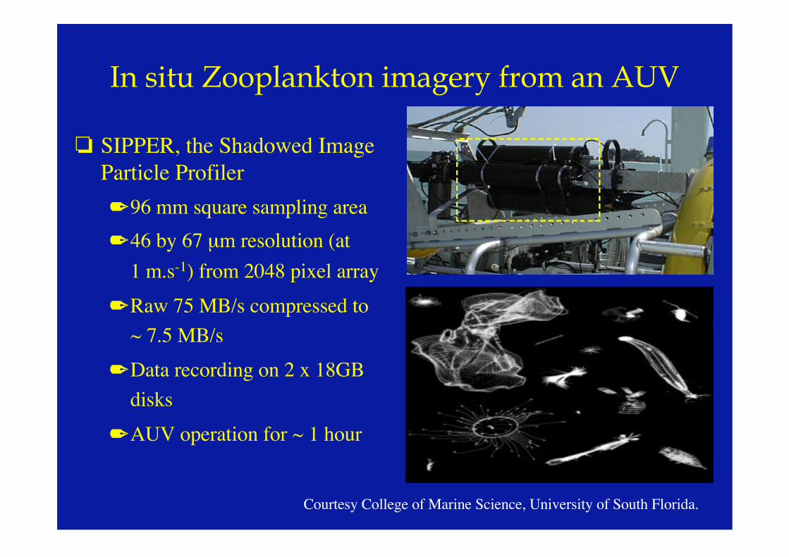
In situ Zooplankton imagery from an AUV

Courtesy College of Marine Science, University of South Florida.

! SIPPER, the Shadowed ImageParticle Profiler"96 mm square sampling area"46 by 67 µm resolution (at1 m.s-1) from 2048 pixel array

"Raw 75 MB/s compressed to~ 7.5 MB/s

"Data recording on 2 x 18GBdisks

"AUV operation for ~ 1 hour

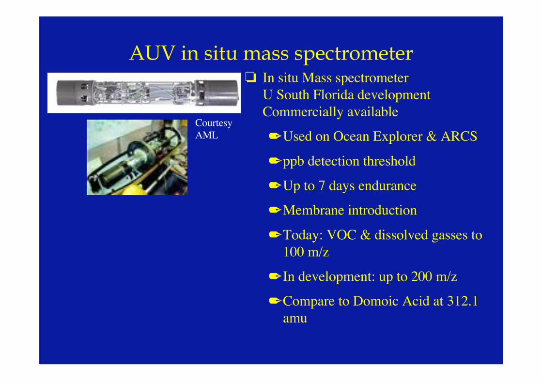
AUV in situ mass spectrometer! In situ Mass spectrometerU South Florida developmentCommercially available

"Used on Ocean Explorer & ARCS

"ppb detection threshold

"Up to 7 days endurance

"Membrane introduction

"Today: VOC & dissolved gasses to100 m/z

" In development: up to 200 m/z

"Compare to Domoic Acid at 312.1amu

CourtesyAML

Examples of Glider & AUV userelevant to study of HABs

! Glider operations off Florida in the Gulf of Mexico

! Studies of small-scale patchiness off Cape Cod,Massachusetts

! Investigation of mixed phytoplankton populations off theScilly Isles, UK

! Hypothesis-testing experiment on krill distribution in theWeddell Sea

! Acoustic fish stock assessment from an AUV

! Flow and turbulence measurements in the coastal ocean

Operation Gulfcast

! “Our goal is to develop anintelligent fleet of coastalSlocum Gliders thatprovide maps of thephysics, bio-optics andbiology on continentalshelves”From a poster by Schofieldet al. (2003)

Data and illustrations courtesy ofDr Oscar Schofield, Rutgers UniversityInstitute of Coastal and Marine Science.

The Tools The Slocum electric gliderfrom Webb Research

Length: 150 cmMass: 52 kgPayload: 5 kgWingspan: 120 cmEnergy: 8MJ at 21˚CPmax: 200 dbarUmax: 0.4 m.s-1

Hydroscat 2

Optical backscatter &fluorescence from dualwavelength HOBI-LabsHydroScat-2

670 & 470 nm excitationBackscatter at 140˚Chlorophyll emission2.5 l volume; 4 kg in air1 W power consumption

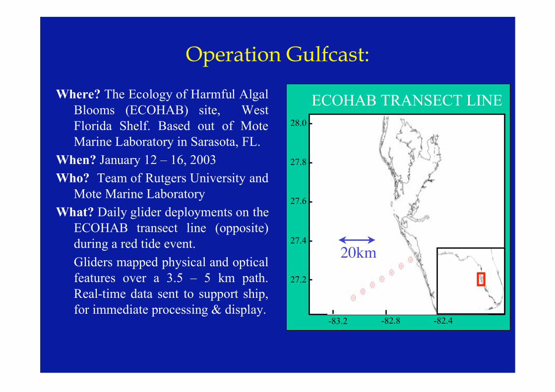
Operation Gulfcast:

Where? The Ecology of Harmful AlgalBlooms (ECOHAB) site, WestFlorida Shelf. Based out of MoteMarine Laboratory in Sarasota, FL.

When? January 12 – 16, 2003Who? Team of Rutgers University andMote Marine Laboratory

What? Daily glider deployments on theECOHAB transect line (opposite)during a red tide event.Gliders mapped physical and opticalfeatures over a 3.5 – 5 km path.Real-time data sent to support ship,for immediate processing & display.

27.4

27.6

27.8

28.0

27.2

-82.8 -82.4-83.2

ECOHAB TRANSECT LINE

20km

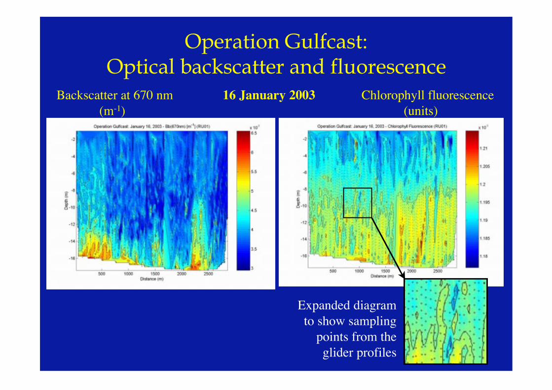
Operation Gulfcast:Optical backscatter and fluorescence

Backscatter at 670 nm 16 January 2003 Chlorophyll fluorescence (m-1) (units)

Expanded diagramto show samplingpoints from theglider profiles

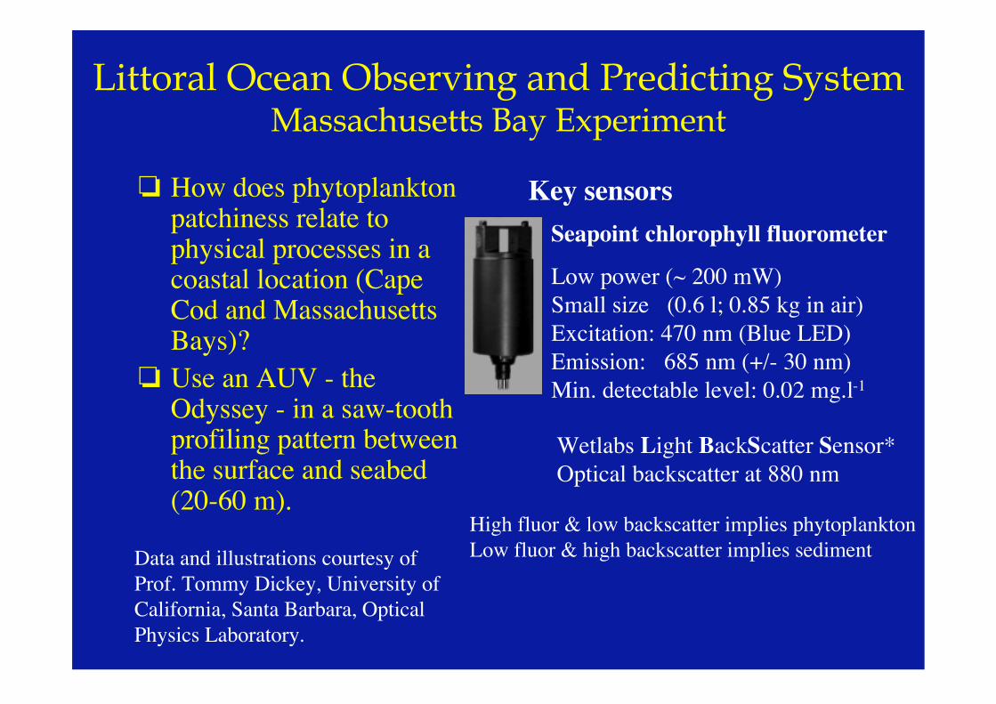
Littoral Ocean Observing and Predicting SystemMassachusetts Bay Experiment

! How does phytoplanktonpatchiness relate tophysical processes in acoastal location (CapeCod and MassachusettsBays)?

! Use an AUV - theOdyssey - in a saw-toothprofiling pattern betweenthe surface and seabed(20-60 m).

Data and illustrations courtesy ofProf. Tommy Dickey, University ofCalifornia, Santa Barbara, OpticalPhysics Laboratory.

Key sensorsSeapoint chlorophyll fluorometer

Low power (~ 200 mW)Small size (0.6 l; 0.85 kg in air)Excitation: 470 nm (Blue LED)Emission: 685 nm (+/- 30 nm)Min. detectable level: 0.02 mg.l-1

Wetlabs Light BackScatter Sensor*Optical backscatter at 880 nm

High fluor & low backscatter implies phytoplanktonLow fluor & high backscatter implies sediment

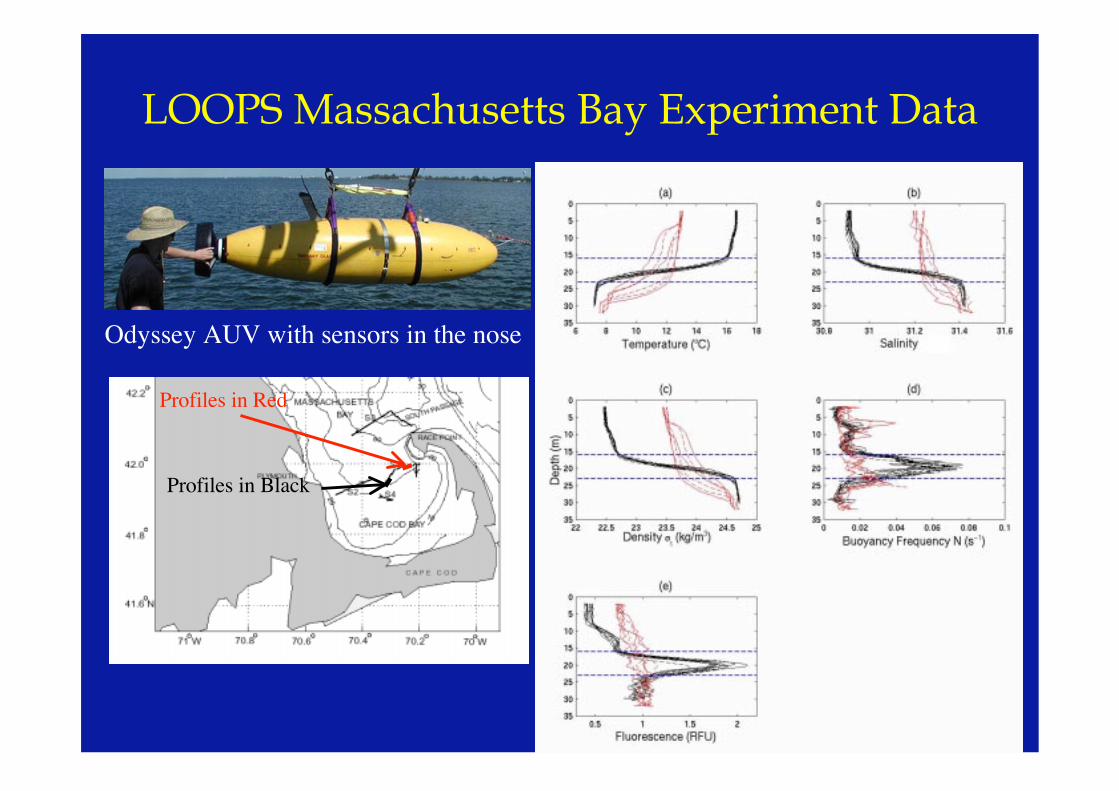
LOOPS Massachusetts Bay Experiment Data

Profiles in Red

Profiles in Black

Odyssey AUV with sensors in the nose

LOOPS Massachusetts Bay Experiment Results

! Chlorophyll profiles well measured with verticalresolution of ~ 0.1 m and horizontal resolution of ~ 120 mat the pycnocline

! Zero crossing of autocorrelation length scale, as observed,was ~ 450 m" AUV profiles with horizontal resolution of ~ 120 m provided>3 samples within this scale, and >12 samples within one period(assuming period ~ 4 x the autocorrelation length scale).

" Apparent scale - 1.8 km - needs correcting for Doppler shift

! Newer optical scattering sensors, e.g. three-wavelength(470,530, 660 nm), three angle (100, 125, 150˚) devicefrom Wetlabs (ECO-VSF3) would provide additionalinformation.

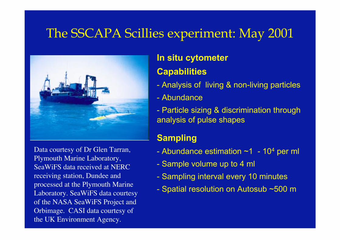
The SSCAPA Scillies experiment: May 2001

In situ cytometer

Capabilities

- Analysis of living & non-living particles

- Abundance

- Particle sizing & discrimination throughanalysis of pulse shapes

Sampling

- Abundance estimation ~1 - 104 per ml

- Sample volume up to 4 ml

- Sampling interval every 10 minutes

- Spatial resolution on Autosub ~500 m

Data courtesy of Dr Glen Tarran,Plymouth Marine Laboratory,SeaWiFS data received at NERCreceiving station, Dundee andprocessed at the Plymouth MarineLaboratory. SeaWiFS data courtesyof the NASA SeaWiFS Project andOrbimage. CASI data courtesy ofthe UK Environment Agency.

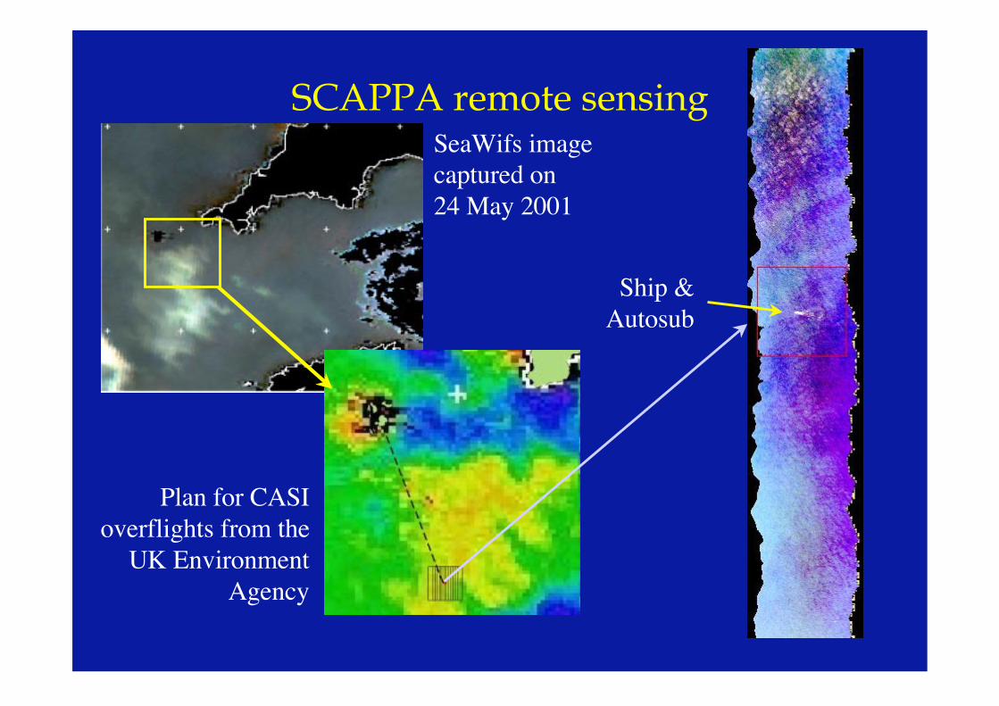
SCAPPA remote sensingSeaWifs imagecaptured on24 May 2001

Plan for CASIoverflights from theUK Environment

Agency

Ship &Autosub

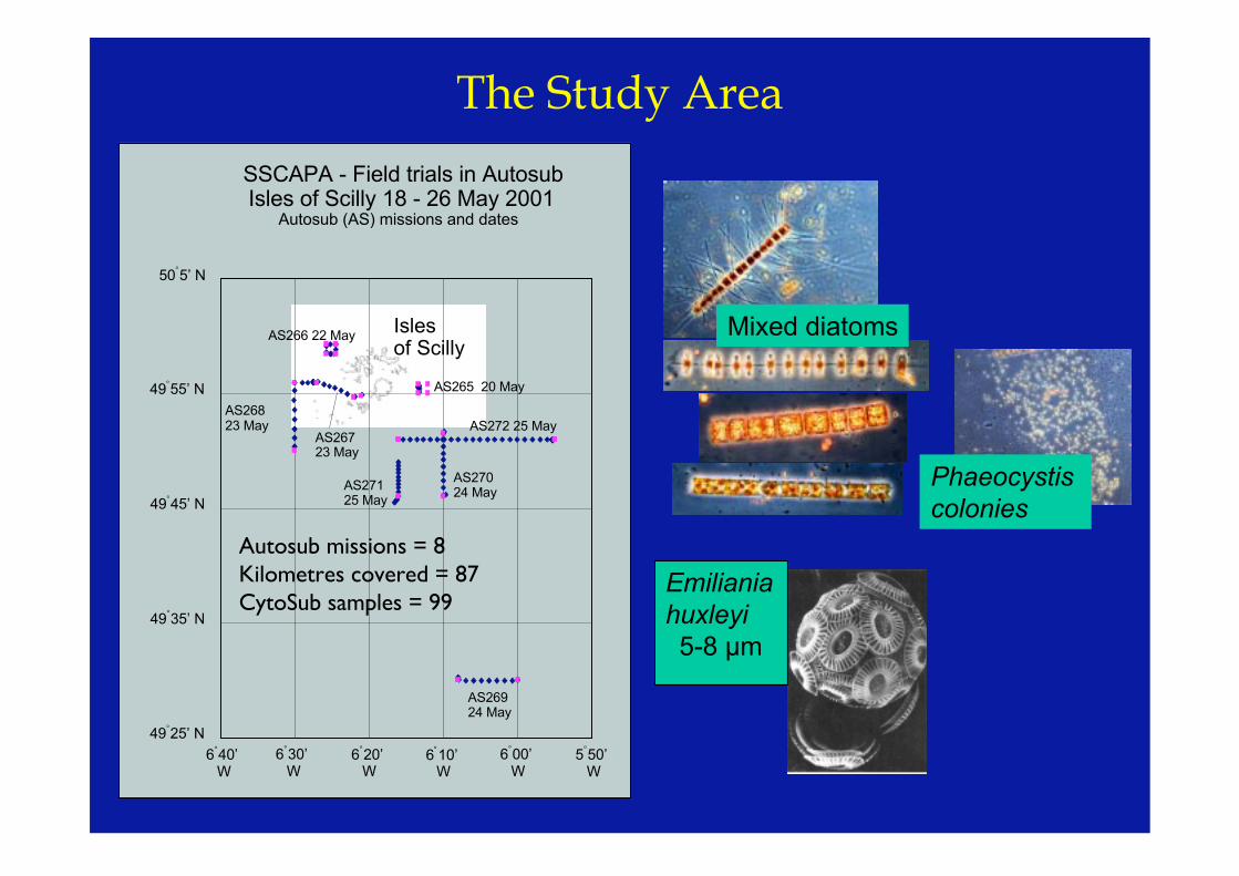
Mixed diatoms

Phaeocystis colonies

Emilianiahuxleyi5-8 µm

50 5’ No

49 25’ No

49 35’ No

49 45’ No

49 55’ No

6 40’ W

o

6 30’ W

o

6 20’ W

o

6 10’ W

o

6 00’ W

o

5 50’W

o

Isles of Scilly

SSCAPA - Field trials in AutosubIsles of Scilly 18 - 26 May 2001

Autosub (AS) missions and dates

AS265 20 May

AS266 22 May

AS26723 May

AS26823 May

AS26924 May

AS27024 MayAS271

25 May

AS272 25 May

Autosub missions = 8Kilometres covered = 87CytoSub samples = 99

The Study Area

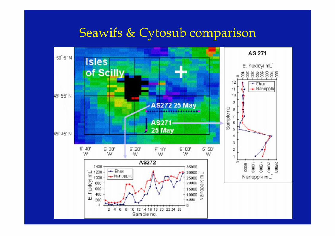
Seawifs & Cytosub comparison

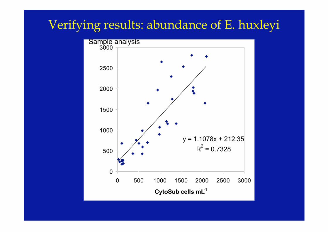
y = 1.1078x + 212.35

R2 = 0.7328

0

500

1000

1500

2000

2500

3000

0 500 1000 1500 2000 2500 3000

CytoSub cells mL-1

Verifying results: abundance of E. huxleyiSample analysis

0

200

400

600

800

1000

1200

1400

1 2 3 4 5 6 7 8 9 10 11 12 13 14 15 16 17 18 19 20 21 22

Sample No.

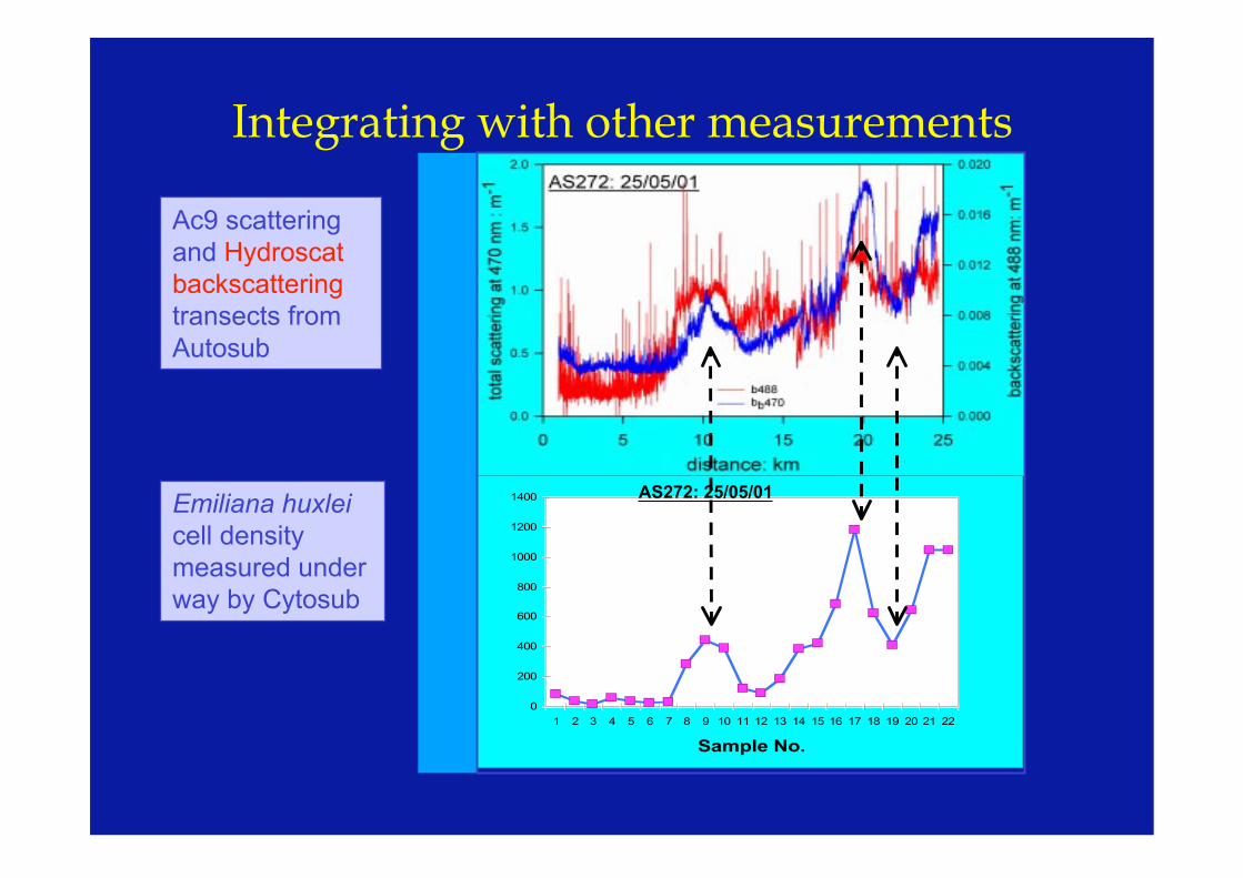
AS272: 25/05/01

Ac9 scatteringand Hydroscatbackscatteringtransects fromAutosub

Emiliana huxleicell densitymeasured underway by Cytosub

Integrating with other measurements

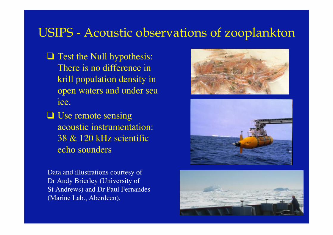
USIPS - Acoustic observations of zooplankton

! Test the Null hypothesis:There is no difference inkrill population density inopen waters and under seaice.

! Use remote sensingacoustic instrumentation:38 & 120 kHz scientificecho sounders

Data and illustrations courtesy ofDr Andy Brierley (University ofSt Andrews) and Dr Paul Fernandes(Marine Lab., Aberdeen).

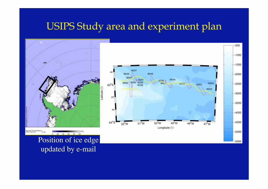
USIPS Study area and experiment plan

Position of ice edgeupdated by e-mail

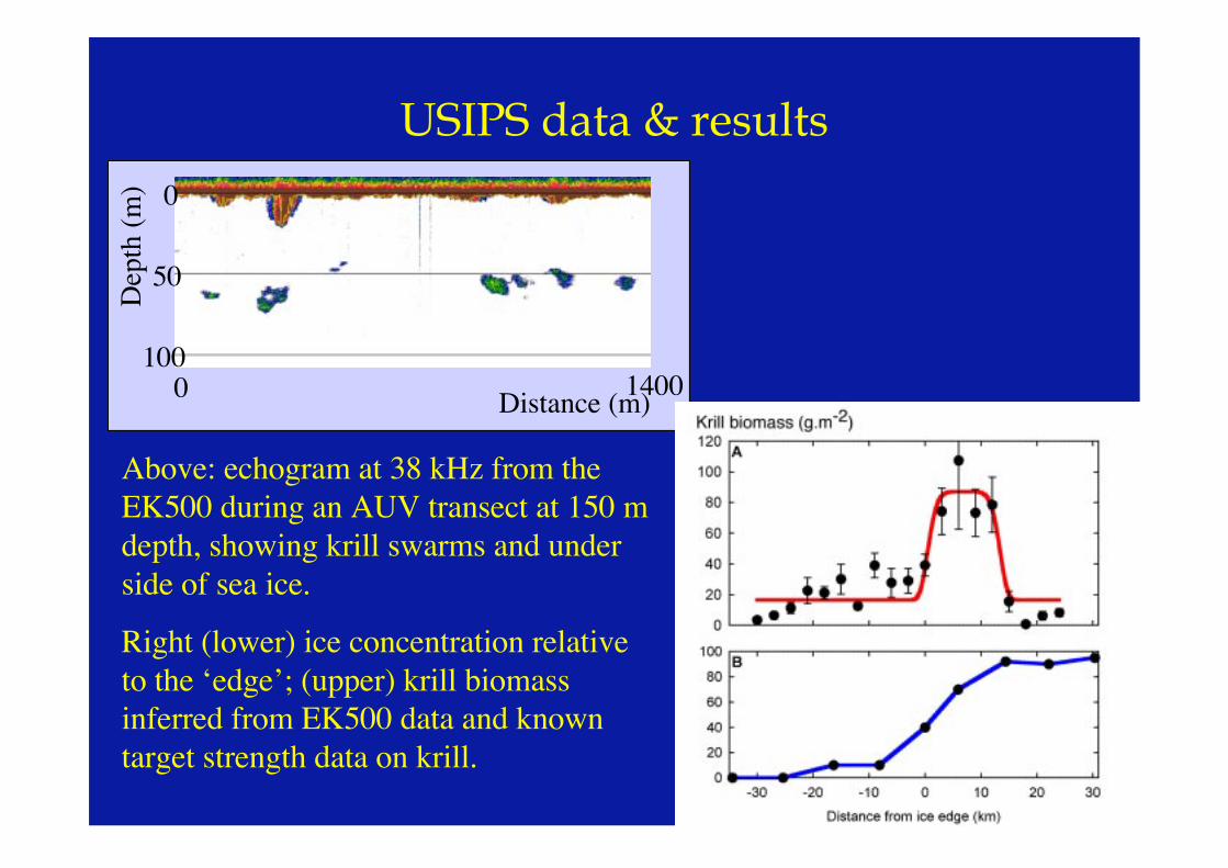
USIPS data & resultsDepth (m) 0

50

100Distance (m)0 1400

Above: echogram at 38 kHz from theEK500 during an AUV transect at 150 mdepth, showing krill swarms and underside of sea ice.

Right (lower) ice concentration relativeto the ‘edge’; (upper) krill biomassinferred from EK500 data and knowntarget strength data on krill.

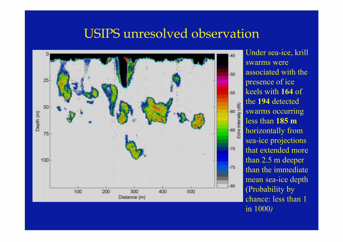
USIPS unresolved observationUnder sea-ice, krillswarms wereassociated with thepresence of icekeels with 164 ofthe 194 detectedswarms occurringless than 185 mhorizontally fromsea-ice projectionsthat extended morethan 2.5 m deeperthan the immediatemean sea-ice depth(Probability bychance: less than 1in 1000)

Sea Ice Thickness from AutosubUnpublished data courtesy Dr Mark Brandon, Open University

Under diffuse ice

Mean thickness is of same magnitude as winter measurements made fromupward-looking sonar in the same area (Strass and Fahrbach, 1998) Thickness is greater than expected from manual ice coring

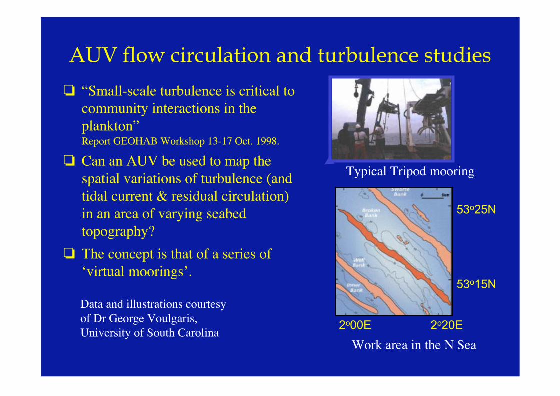
AUV flow circulation and turbulence studies

! “Small-scale turbulence is critical tocommunity interactions in theplankton”Report GEOHAB Workshop 13-17 Oct. 1998.

! Can an AUV be used to map thespatial variations of turbulence (andtidal current & residual circulation)in an area of varying seabedtopography?

! The concept is that of a series of‘virtual moorings’.

Data and illustrations courtesyof Dr George Voulgaris,University of South Carolina

53o25N

53o15N

2o00E 2o20E

Work area in the N Sea

Typical Tripod mooring

Data acquisition and experiment plan

1. 1200 kHz ADCP 1Hz at 10 cm verticalresolution2. 300 kHz ADCP for vehicle navigation3. ADV Point measurement at 16 Hz4. 200 kHz collision avoidance sonar5. 1.75 MHz ping-to-ping coherent Doppler,sub-cm resolution

12

34 5

SWNE

2.12

2.14

2.16

2.18

2.2

2.22

53.2753.28

53.2953.3

53.3153.3

40

30

20

10

0

Latitude (degs)

AUTOSUB Terrain Following Mission N. Sea

Longitude (degs)

Dis

tanc

e fr

om s

ea s

urfa

ce (

m)

Start Point

Surfacing for GPSposition fixing

Terrain Following

Terrain following mission at 4 m above seabed covering 162 km

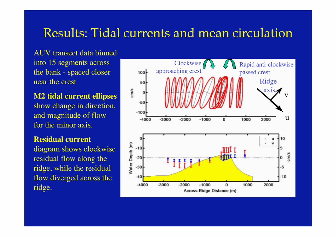
Results: Tidal currents and mean circulationAUV transect data binnedinto 15 segments acrossthe bank - spaced closernear the crest

M2 tidal current ellipsesshow change in direction,and magnitude of flowfor the minor axis.

Residual currentdiagram shows clockwiseresidual flow along theridge, while the residualflow diverged across theridge.

Clockwiseapproaching crest

Rapid anti-clockwisepassed crest

u

v

Ridge axis

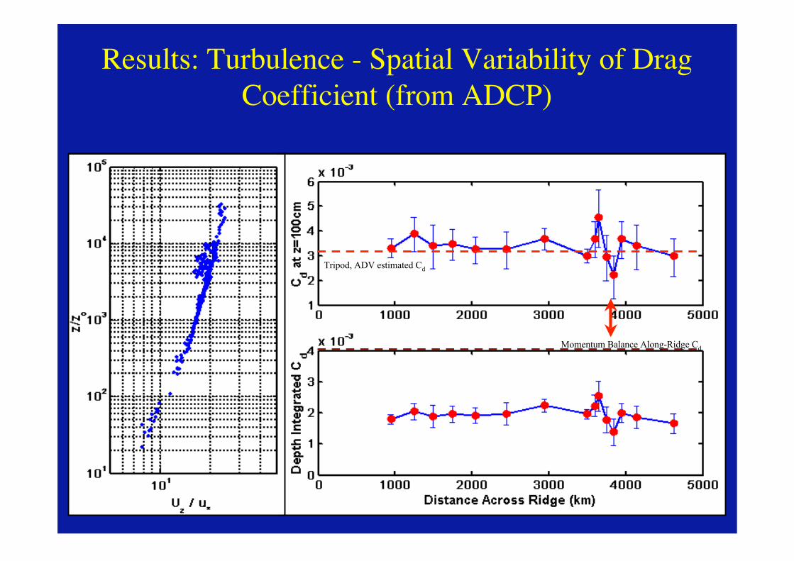
Results: Turbulence - Spatial Variability of DragCoefficient (from ADCP)

Momentum Balance Along-Ridge Cd

Tripod, ADV estimated Cd

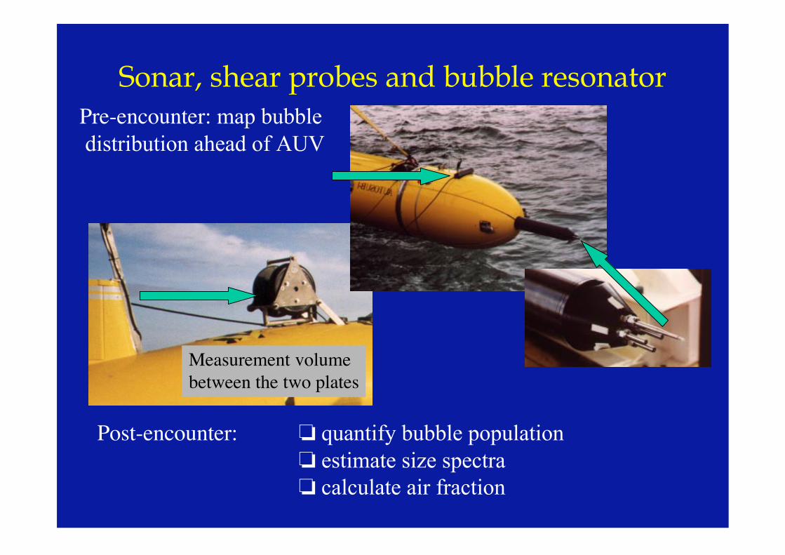
Sonar, shear probes and bubble resonator

Measurement volumebetween the two plates

Post-encounter: ! quantify bubble population ! estimate size spectra ! calculate air fraction

Pre-encounter: map bubble distribution ahead of AUV

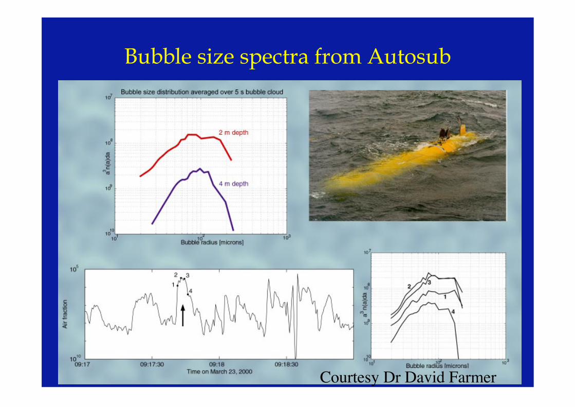
Bubble size spectra from Autosub

Courtesy Dr David Farmer

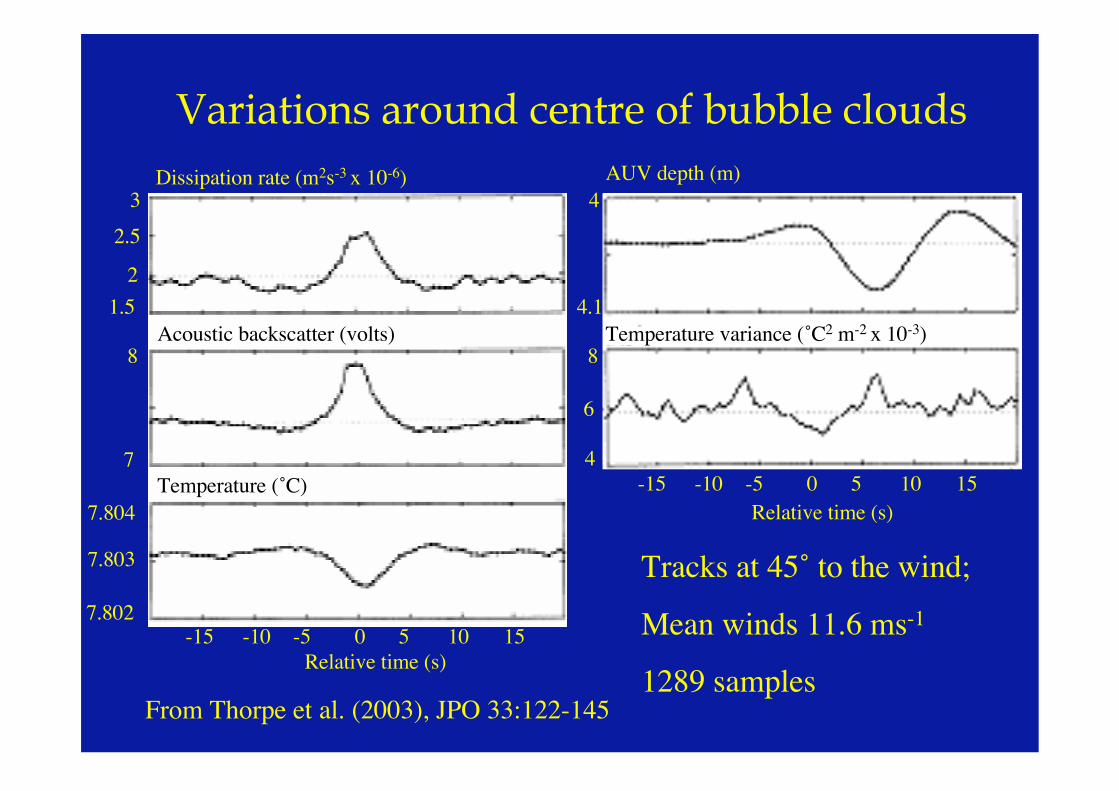
Variations around centre of bubble clouds

From Thorpe et al. (2003), JPO 33:122-145

Tracks at 45˚ to the wind;

Mean winds 11.6 ms-1

1289 samples

Dissipation rate (m2s-3 x 10-6)

Acoustic backscatter (volts)

Temperature (˚C)

AUV depth (m)

Temperature variance (˚C2 m-2 x 10-3)

3

2.5

21.5

8

7

7.804

7.803

7.802

4

4.1

8

6

40 5 10 15-5-10-15

0 5 10 15-5-10-15Relative time (s)

Relative time (s)

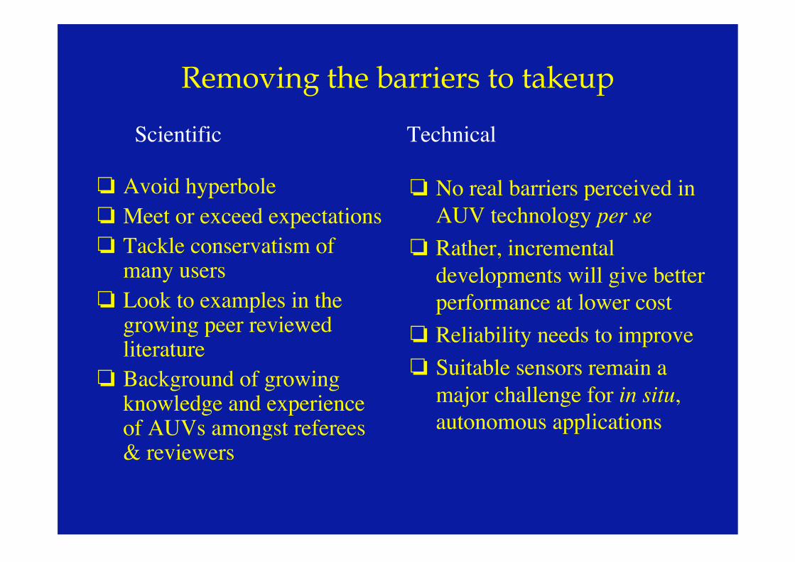
Removing the barriers to takeup

! Avoid hyperbole! Meet or exceed expectations! Tackle conservatism ofmany users

! Look to examples in thegrowing peer reviewedliterature

! Background of growingknowledge and experienceof AUVs amongst referees& reviewers

! No real barriers perceived inAUV technology per se

! Rather, incrementaldevelopments will give betterperformance at lower cost

! Reliability needs to improve! Suitable sensors remain amajor challenge for in situ,autonomous applications

Scientific Technical

Removing the barriers to takeup

! High cost of large & medium-sized AUVs is a seriousbarrier.

! Technology advances leadingto smaller, yet capablevehicles

! Competition driving price-performance improvements

! Service providers areemerging

! Sensor manufacturers areseeing AUVs as potentialmarket

! Move to smaller vehicles toreduce support team andinfrastructure size

! Reduce dependence onsupport ships

! Work towards acceptance ofshore-based missionse.g. develop agreedprotocols, codes of practice

! Work with risk management/ insurance professionals toavoid potential threats

Economic Logistical

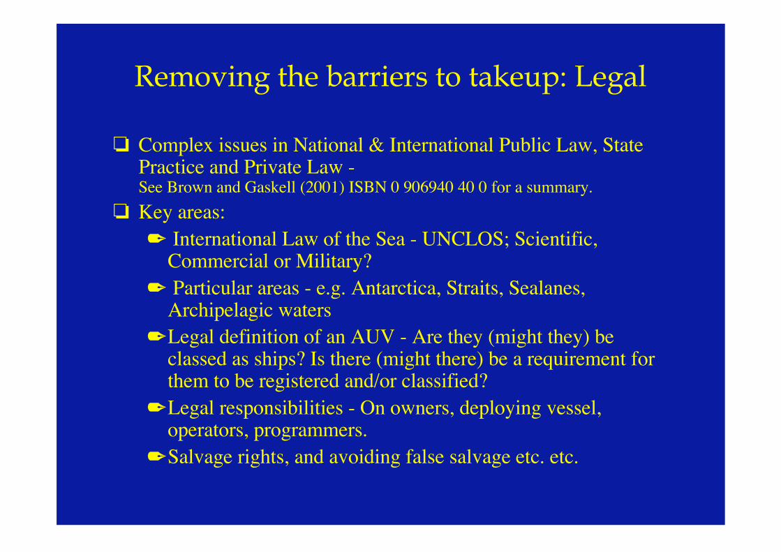
Removing the barriers to takeup: Legal

! Complex issues in National & International Public Law, StatePractice and Private Law -See Brown and Gaskell (2001) ISBN 0 906940 40 0 for a summary.

! Key areas:" International Law of the Sea - UNCLOS; Scientific,Commercial or Military?

" Particular areas - e.g. Antarctica, Straits, Sealanes,Archipelagic waters

"Legal definition of an AUV - Are they (might they) beclassed as ships? Is there (might there) be a requirement forthem to be registered and/or classified?

"Legal responsibilities - On owners, deploying vessel,operators, programmers.

"Salvage rights, and avoiding false salvage etc. etc.

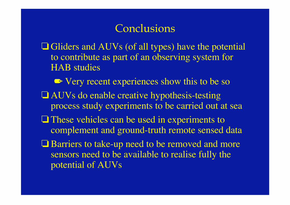
Conclusions

!Gliders and AUVs (of all types) have the potentialto contribute as part of an observing system forHAB studies" Very recent experiences show this to be so

!AUVs do enable creative hypothesis-testingprocess study experiments to be carried out at sea

! These vehicles can be used in experiments tocomplement and ground-truth remote sensed data

! Barriers to take-up need to be removed and moresensors need to be available to realise fully thepotential of AUVs