18.783 Elliptic Curves Spring 2013Lecture #10 03/12/2013

Andrew V. Sutherland

10.1 The discrete logarithm problem

In its most standard form, the discrete logarithm problem (DLP) is stated as follows:

Given α ∈ G and β ∈ 〈α〉, find the least positive integer x such that αx = β.

In additive notation, we want xα = β. In any case, we call x the discrete logarithm of βwith respect to the base α, denoted by log 1

α β.We can formulate a slightly stronger version of the problem:

Given α, β ∈ G, compute logα β if β ∈ 〈α〉, otherwise, report that β 6∈ 〈α〉.

This can be a significantly harder problem. For example, say we are using a randomized (LasVegas) algorithm. If β lies in 〈α〉 then we are guaranteed to eventually find logα β, but ifnot, we will never find it and it may be impossible to tell whether we are just very unluckyor β 6∈ 〈α〉. On the other hand, with a deterministic algorithm such as the baby-stepsgiant-steps method, we can unequivocally determine whether β lies in 〈α〉 or not.

There is also a generalization called the extended discrete logarithm:

Given α, β ∈ G, determine the least positive integer y such that βy ∈ 〈α〉, andthen output the pair (x, y), where x = logα β

y.

This yields positive integers x and y satisfying βy = αx, where we minimize y first and xsecond. Note that there is always a solution: in the worst case x = |α| and y = |β|.

Example 10.1. Suppose G = F×101. Then log3 37 = 24, since 324 ≡ 37 mod 101.

Example 10.2. Suppose G = F+101. Then log3 37 = 46, since 46 · 3 = 37 mod 101.

Both of these examples involve groups where the discrete logarithm is easy to compute(and not just because 101 is a small number), but for very different reasons. In Example 10.1we are working in a group of order 100 = 22·52. As we will see in this lecture, when the grouporder is a product of small primes (i.e. smooth), it is easy to compute discrete logarithms.In Example 10.2 we are working in a group of order 101, which is prime. In terms of thegroup order, this represents the hardest possible case. But in fact it is very easy to computediscrete logarithms in the additive group of a finite field! All we need to do is compute theinverse of 3 modulo 101 (which is 34) and multiply by 37. This is a small example, buteven if the field size is very large, we can use the extended Euclidean algorithm to computeinverses in quasi-linear time.

So while the DLP is generally considered a “hard problem”, it really depends on whichgroup we are talking about. In the case of the additive group of a finite field the problem iseasier not because the group itself is different in any group-theoretic sense, but because itis embedded in a field. This allows us to perform operations on group elements beyond the

1We will primarily use additive notation, but stick with the multiplicative terminology (hence the wordlogarithm), which is traditional; most of the early work on discrete logarithms was done in the multiplicativegroup of a finite field.

1

standard group operation, which is in some sense “cheating”. Note that if the Euclideanalgorithm were only allowed to use addition and subtraction it would take exponential time.

Even when working in the multiplicative group of a finite field, where the DLP is believedto be much harder, we can do substantially better than in a generic setting. As we shall see,there sub-exponential time algorithms for this problem, whereas in the generic case onlyexponential time algorithms exist, as we will prove in the next lecture. The reason we cando better than in the generic case again arises from the fact that the group in question isembedded in a larger algebraic structure.

10.2 Generic group algorithms

To make formal the notion of “not cheating”, we define a generic group algorithm (or just ageneric algorithm) to be one that interacts with the group G using a black box (also calledan oracle), via the following interface (think of a black box with four buttons, two inputslots, and one output slot ):

1. identity: output the identity element.

2. invert: given input α, output α−1 (or −α, in additive notation).

3. composition: given inputs α and β, output αβ (or α+ β, in additive notation).

4. random: output a uniformly distributed random element α ∈ G.

All group elements processed by the black box are represented as bit-strings of lengthk = O(log |G|). Some models for generic group algorithms also include a black box operationfor testing equality of group elements, but we will instead assume that group elements areuniquely identified ; this means that there is an injective identification map G → 0, 1ksuch that all inputs and outputs to the black box are bit-strings in 0, 1k that correspondto images of group elements under this map. With uniquely identified group elements wecan test equality by comparing bit-strings, which does not involve the black box.2

The black box may use any identification map (including one chosen at random). Ageneric algorithm is not considered correct unless it works no matter what the identificationmap is. We have already seen several examples of generic group algorithms, includingexponentiation algorithms, fast order algorithms, and the baby-steps giant-steps method.

We measure the time complexity of a generic group algorithm by counting group op-erations, the number of interactions with the black box. This metric has the virtue ofbeing independent of the actual software and hardware implementation, allowing one tomake comparisons the remain valid even as technology improves. But if we want to get acomplete measure of the complexity of solving a problem in a particular group, we need tomultiply the group operation count by the bit-complexity of each group operation, whichof course depends on the black box. To measure the space complexity, we count the totalnumber of group identifiers stored at any one time (i.e. the maximum number of groupidentifiers the algorithm ever has to remember).

These complexity metrics do not account for any other work done by the algorithm. Ifthe algorithm wants to compute a trillion digits of pi, or factor some huge integer, it caneffectively do that “for free”. But the implicit assumption is that the cost of any auxiliarycomputation is at worst proportional to the number of group operations, which is true ofall the algorithms we will consider.

2We can also sort bit-strings or index them with a hash table or other data structure; this is essential toan efficient implementation of the baby-steps giant-steps algorithm.

2

10.3 Generic algorithms for the discrete logarithm problem

We now consider generic algorithms for the discrete logarithm problem. We shall assumethroughout that N = |α| is known. This is a reasonable assumption, since there is a genericalgorithm to compute N using o(

√N) group operations [5], which is strictly less than the

complexity of any of the generic algorithms we consider (at least in the worst case, when Nis prime). Indeed, we will prove an Ω(

√N) lower bound for prime N in the next lecture.

The cyclic group 〈α〉 is isomorphic to the additive group Z/NZ, where N is the orderof α. In the context of generic group algorithms, we may as well assume 〈α〉 is Z/NZ,generated by α = 1, since every cyclic group of order N looks the same when it is hiddenin a black box. Of course with the black box picking arbitrary group identifiers, we cannotactually tell which integer x in Z/NZ corresponds to a particular group element β; indeed,x is precisely the discrete logarithm of β that we wish to compute!

Thus computing discrete logarithms amounts to explicitly computing the isomorphismfrom 〈α〉 to Z/NZ. Computing the isomorphism in the reverse direction is easy: this is justexponentiation. Thus we have (in multiplicative notation):

Z/NZ ' 〈α〉x→ αx

logα β ← β

Cryptographic applications of the discrete logarithm problem rely on the fact that it iseasy to compute β = αx but hard (in general) to compute x = logα β.

10.3.1 Linear search

Starting form α, computeα, 2α, 3α, . . . ,mα = β,

and then output m (or if we reach m > N , report that β 6∈ 〈α〉). This uses at most Ngroup operations, and the average over all inputs is N/2 group operations.

We mention this algorithm only for the sake of comparison. Its time complexity is notattractive, but it is very space-efficient: it only needs to store one group element, in additionto the inputs α and β.

10.3.2 Baby-steps giant-steps

Pick positive integers r and s such that rs > N , and then compute:

baby steps: 0, α, 2α, 3α, . . . , (r − 1)α,giant steps: β, β − rα, β − 2rα, . . . , β − (s− 1)rα,

A collision occurs when we find a baby step that is equal to a giant step. We then have

iα = β − jrα,

for some nonnegative integers i < r and j < s. If i = j = 0, then β is the identity andlogα β = N . Otherwise,

logα β = i+ jr.

Typically the baby steps are stored in a lookup table, allowing us to check for a collisionas each giant step is computed, so we don’t necessarily need to compute all the giant steps.

3

We can easily detect β 6∈ 〈α〉, since every integer in [1, N ] can be written in the form i+ jrwith 0 ≤ i < r and 0 ≤ j < s. If we do not find a collision, then β 6∈ 〈α〉.

The baby-steps giant-steps algorithm uses r+s group operations, which is O(√N) if we

choose r ≈ s. It requires space for r group elements (the baby steps), which is also O(√N)

but can be made smaller if are willing to increase the running time by making s larger. Sothere is a trade-off between time and space.

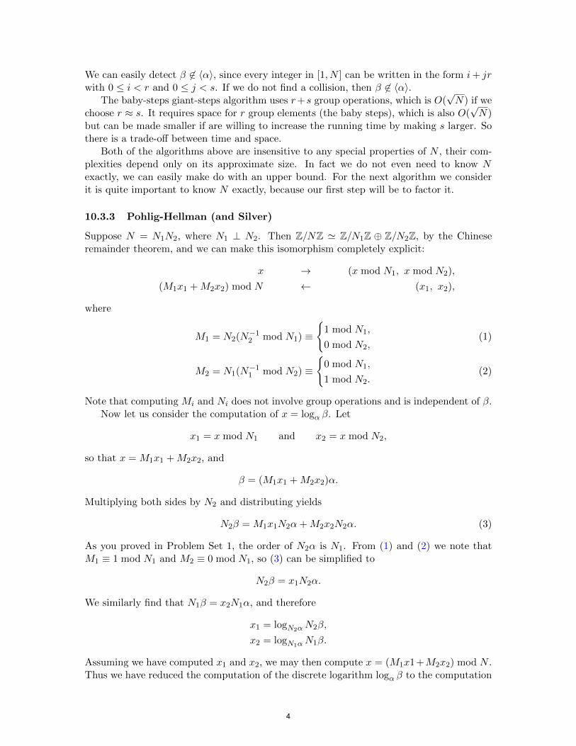
Both of the algorithms above are insensitive to any special properties of N , their com-plexities depend only on its approximate size. In fact we do not even need to know Nexactly, we can easily make do with an upper bound. For the next algorithm we considerit is quite important to know N exactly, because our first step will be to factor it.

10.3.3 Pohlig-Hellman (and Silver)

Suppose N = N1N2, where N1 ⊥ N2. Then Z/NZ ' Z/N1Z ⊕ Z/N2Z, by the Chineseremainder theorem, and we can make this isomorphism completely explicit:

x → (x mod N1, x mod N2),

(M1x1 +M2x2) mod N ← (x1, x2),

where

M1 = N2(N−12 mod N1) ≡

1 mod N1,

(1)0 mod N2,

M2 = N1(N−1 0 mod N1,1 mod N2) ≡

(2)

1 mod N2.

Note that computing Mi and Ni does not involve group operations and is independent of β.Now let us consider the computation of x = logα β. Let

x1 = x mod N1 and x2 = x mod N2,

so that x = M1x1 +M2x2, and

β = (M1x1 +M2x2)α.

Multiplying both sides by N2 and distributing yields

N2β = M1x1N2α+M2x2N2α. (3)

As you proved in Problem Set 1, the order of N2α is N1. From (1) and (2) we note thatM1 ≡ 1 mod N1 and M2 ≡ 0 mod N1, so (3) can be simplified to

N2β = x1N2α.

We similarly find that N1β = x2N1α, and therefore

x1 = logN2αN2β,

x2 = logN1αN1β.

Assuming we have computed x1 and x2, we may then compute x = (M1x1+M2x2) mod N .Thus we have reduced the computation of the discrete logarithm logα β to the computation

4

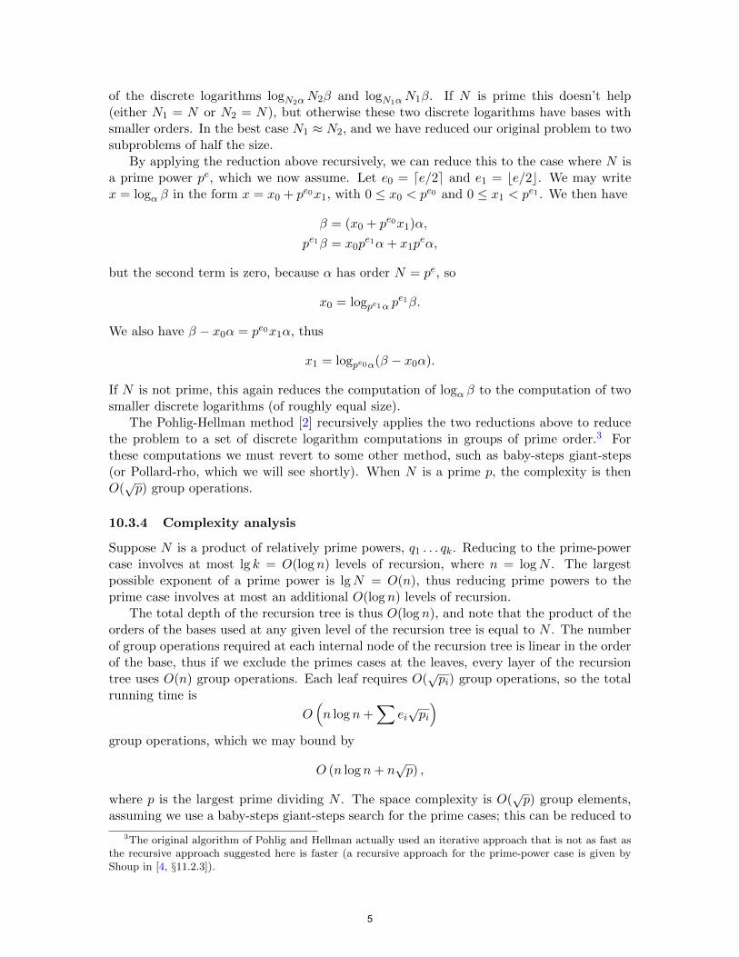
of the discrete logarithms logN2αN2β and logN1αN1β. If N is prime this doesn’t help(either N1 = N or N2 = N), but otherwise these two discrete logarithms have bases withsmaller orders. In the best case N1 ≈ N2, and we have reduced our original problem to twosubproblems of half the size.

By applying the reduction above recursively, we can reduce this to the case where N isa prime power pe, which we now assume. Let e0 = de/2e and e1 = be/2c. We may writex = logα β in the form x = x0 + pe0x1, with 0 ≤ x0 < pe0 and 0 ≤ x1 < pe1 . We then have

β = (x0 + pe0x1)α,

pe1β = x0pe1α+ x1p

eα,

but the second term is zero, because α has order N = pe, so

x0 = logpe1α pe1β.

We also have β − x0α = pe0x1α, thus

x1 = logpe0α(β − x0α).

If N is not prime, this again reduces the computation of logα β to the computation of twosmaller discrete logarithms (of roughly equal size).

The Pohlig-Hellman method [2] recursively applies the two reductions above to reducethe problem to a set of discrete logarithm computations in groups of prime order.3 Forthese computations we must revert to some other method, such as baby-steps giant-steps(or Pollard-rho, which we will see shortly). When N is a prime p, the complexity is thenO(√p) group operations.

10.3.4 Complexity analysis

Suppose N is a product of relatively prime powers, q1 . . . qk. Reducing to the prime-powercase involves at most lg k = O(log n) levels of recursion, where n = logN . The largestpossible exponent of a prime power is lgN = O(n), thus reducing prime powers to theprime case involves at most an additional O(log n) levels of recursion.

The total depth of the recursion tree is thus O(log n), and note that the product of theorders of the bases used at any given level of the recursion tree is equal to N . The numberof group operations required at each internal node of the recursion tree is linear in the orderof the base, thus if we exclude the primes cases at the leaves, every layer of the recursiontree uses O(n) group operations. Each leaf requires O(

√pi) group operations, so the total

running time is

O(n log n+

∑ei√pi

group operations, which we may bound by

)

O (n log n+ n√p) ,

where p is the largest prime dividing N . The space complexity is O(√p) group elements,

assuming we use a baby-steps giant-steps search for the prime cases; this can be reduced to

3The original algorithm of Pohlig and Hellman actually used an iterative approach that is not as fast asthe recursive approach suggested here is faster (a recursive approach for the prime-power case is given byShoup in [4, §11.2.3]).

5

O(1) using the Pollard-rho method (which is the next algorithm we will consider), but thisresults in a probabilistic (Las Vegas) algorithm, whereas the basic Pohlig-Hellman approachis completely deterministic.

The Pohlig-Hellman algorithm can be extremely efficient when N is composite; if N issufficiently smooth it runs in quasi-linear time (computing discreate logarithms in a group oforder 101000 takes almost no time at all). This underscores the importance of using groups ofprime or near-prime order in any cryptographic application based on the discrete logarithmproblem. This is one of the main motivations for efficient point-counting algorithms forelliptic curves: we really want to know exactly what the group order is.

10.4 Randomized algorithms for the discrete logarithm problem

So far we have only considered deterministic algorithms. We will not achieve a better timecomplexity bound with randomization, but we can achieve a much better space complexity;this also makes it much easier to parallelize the algorithm, which is crucial for large-scalecomputations (one can construct a parallel version of the baby-steps giant-steps algorithm,but detecting collisions is more complicated and requires a lot of communication).

10.4.1 The birthday paradox

Recall what the birthday paradox tells us about collision frequency: if we drop Ω(√N) balls

randomly into O(N) bins then the probability that some bin contains more than one ballis bounded below by some nonzero constant that we can make arbitrarily close to 1. Givenβ√∈ 〈α〉, the baby-steps giant-steps method for computing logα β can be viewed as dropping

2N balls that are linear combinations of α and β (the baby steps are linear combinationsof α alone) into N bins corresponding to the elementd of 〈α〉. Of course these balls are notdropped randomly, they are dropped a

But√in a pattern that guarantees collision.

if we instead just computed 2N linear combinations of α and β at random, thebirthday paradox tells us that we would still have a good chance of finding a collision(better than 50/50, in fact). The main problem with this approach is that in order to findthe collision we might need to keep track of all the linear combinations we have computed,which would take a lot of space. In order to take advantage of the birthday paradox in away that uses less space we need to be a bit more clever.

10.4.2 Random walks on a graph

Let us now view the group 〈α〉 as the vertext set V of a graph. Suppose we use a randomfunction f : V → V to construct a walk from a random starting point v0 as follows:

v1 = f(v0)

v2 = f(v1)

v3 = f(v2)

...

Since f is a function, if we ever repeat a vertex, say vρ = vλ for some ρ > λ, we will bepermanently stuck in a cycle, since we then have f(vρ+i) = f(vλ+i) for all i ≥ 0. This is agood thing, because once we are in this cycle every step corresponds to a collision (a pair

6

of vertices with different indices in our random walk that correspond to the same groupelement). Note that V is finite, so we must eventually hit a cycle.

Our random walk thus consists of two parts, a path from v0 to the vertex vλ, the firstvertex that is visited more than once, and a cycle consisting of the vertices vλ, vλ+1, . . . , vρ−1.The can be visualized as a path in the shape of the Greek letter ρ, which explains the nameof the ρ-method we wish to consider.

A collision doesn’t necessarily tell us anything on its own, but if we augment the func-tion f appropriately, it will. We will construct f so that the vertices in our random walkcorrespond to linear combinations aα + bβ whose coefficients a and b we know. But let usfirst compute the expected number of steps a random walk takes to reach its first collision.

Theorem 10.3. Let V be a finite set. For any v0 ∈ V , the expected value of ρ for a walkfrom v0 defined by a random function f : V → V is

E[ρ] ∼√πN/2,

as the cardinality N of V tends to infinity.

This theorem was stated in lecture without proof; we now give an elementary proof.

Proof. Let Pn = Pr[ρ > n]. We have P0 = 1 and P1 = (1− 1/N), and in general

Pn =( 1

1−N

)(1− 2

N

)· · ·(

1− n

N

)=

n∏i=1

(1− i

N

)for any n < N (and Pn = 0 for n ≥ N). We compute the expectation of ρ as

N−1

E[ρ] =∑

n · Pr[ρ = n]n=1

N−1

= nn=1

· (Pn−1 − Pn),

= 1(

∑P0 − P1) + 2(P1 − P2) + . . .+ n(Pn−1 − Pn)

N−1

=n

∑Pn

=0

− nPn. (4)

In order to determine the asymptotic behavior of E[ρ] we need tight bounds on Pn. Usingthe fact that log(1− x) < −x for 0 < x < 1, we obtain an upper bound on Pn:

iPn =

(∑nexp log

i

(1

=1

−N

))

< exp

(1−

n

∑ni

Ni=1

)

< exp(− 2

2N

).

7

To establish a lower bound, we use the fact that log(1− x) > −x− x2 for 0 < x < 1 , which2can be verified using the Taylor series expansion for log(1− x).

Pn = exp

(∑nlog

i=1

( i1−

N

))

> exp

(n

−∑i=1

( iN

+i2

.N2

))

We now let M = N3/5 and assume n < M . In this range we have

∑ni=1

( iN

+i2

N2

)<

n∑i=1

( iN

+N−45

n2 + n

)<

1

+N−2N

5

n2<

1+

2N 2N−

25 +N−

15

n2<

1

+ 2N−2N

5 ,

which implies

Pn > exp(−n2

2N

)exp

(−2N−

15

)=(1 + o(1)

)exp

(−n2.

2N

We now return to the computation of E[ρ]. From (4

)) we have

b

E[ρ] =n

∑Mc N−1

Pn +∑

Pn + o(1) (5)=0 n=dMe

2where the error term comes from nPn < n exp

(−n = o(1) (we use o(1) to denote any2Nterm whose absolute value tends to 0 as N →∞). The

)second sum is negligible, since

N∑−1 2

Pn < N exp

n dMe

( M−=

2N

)= N exp

( 1−2N−

15

= o(1).

)(6)

8

For the first sum we have

d∑Me d∑Me ( ) ( n2Pn = 1 + o(1) exp

n=0 n=0

−2N

)= (1 + o(1))

∫ ∞ 2

e−x

0

2N dx+O(1)

= (1 + o(1))√ ∞

2N

∫eu

2du+O(1)

0

= (1 + o(1))√

2N(√√ π/2)

= (1 + o(1)) πN/2. (7)

Plugging (6) and (7) in to (5) yields the desired result.

Remark 10.4. One can also show E[λ] = E[σ] = 12E[ρ] =

√πN/8, where σ = ρ− λ is the

length of the cycle.

In the baby-steps giant-steps algorithm (BSGS), if we assume that the discrete logarithmis uniformly distributed over [1, N ], then we should use

√N/2 baby steps and expect to

find the discrete logarithm after√N/2 giant steps, on average, using a total of

√√ 2N groupoperations. But note that π/2 ≈ 1.25 is less than

√2 ≈ 1.41, so we may hope to compute

discrete logarithms faster than BSGS (on average) by simulating a random walk. Of coursethe worst-case running time for BSGS is better, we will never need more than

√2N giant

steps, but with a random walk the (astronomically unlikely) worst case is N steps.

10.5 Pollard-ρ Algorithm

We now present the Pollard-ρ algorithm for computing logα β. As noted earlier, a collisionin a random walk is useful to us only if we know how to express the colliding group elementsas (independent) linear combinations of α and β. Thus we extend the function f : G → Gthat defines our random walk to a function

f : (Z/NZ)2 ×G→ (Z/NZ)2 ×G,′

which, given (a, b, γ) such that αaβb′

= γ, outputs some (a′, b′, γ′) such that αa βb = γ′.There are several ways to define such a function f , one of which is the following. First

fix r distinct group elements δi = ciα + diβ for some randomly chosen ci, di ∈ Z/NZ. Inorder to simulate a random walk, we don’t want r to be too small: empirically a value ofaround 20 works well [6]. Then define f(a, b, γ) = (a + ci, b + di, γ + δi) where i = h(γ) isdetermined by a randomly chosen hash function

h : G→ 1, . . . , r.

In practice we don’t choose h randomly, we just need the preimages h−1(i) to partition Ginto r subsets of roughly equal size (for example, we might just reduce the integer corre-sponding to the bit-string that uniquely represents γ modulo r, assuming that these integersare roughly equidistributed mod r).4

4Note the importance of unique identifiers. We must be sure that γ is always hashed to to the samevalue. Using a non-unique representation such as projective points on an elliptic curve will not achieve this.

9

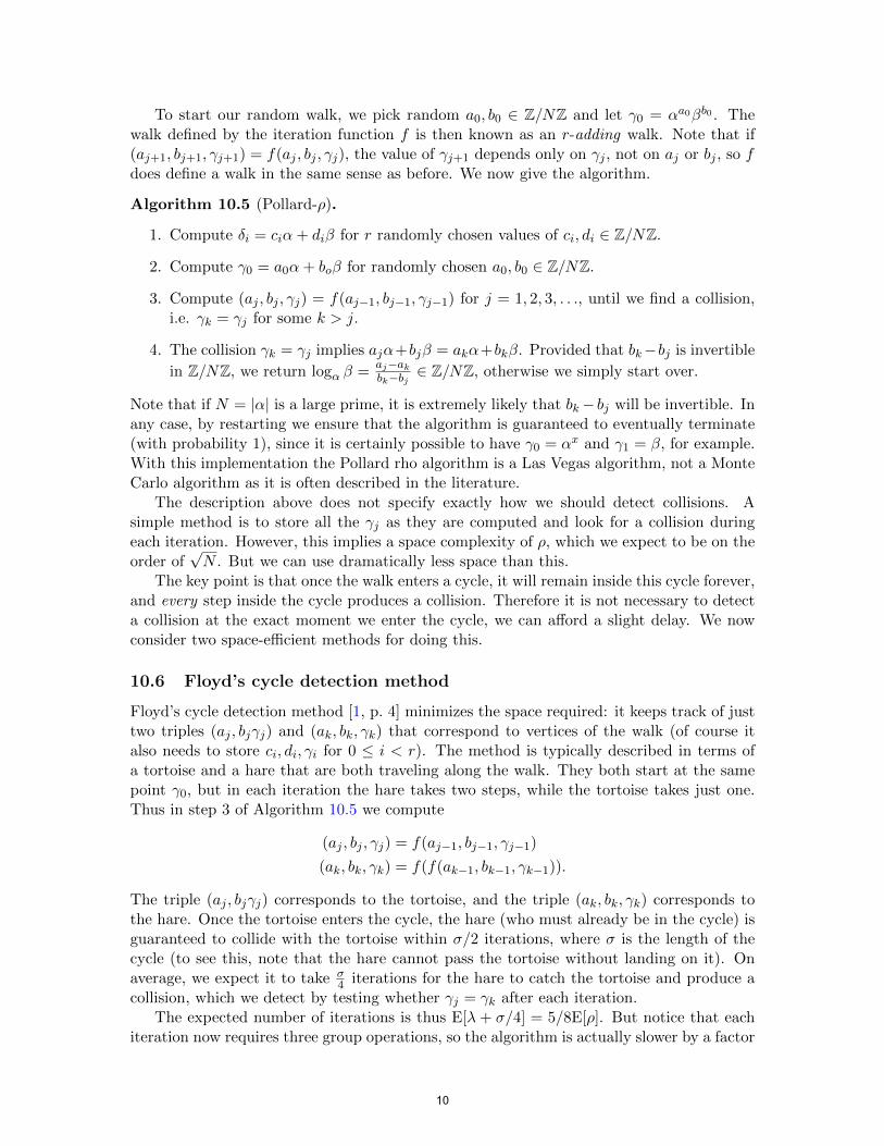
To start our random walk, we pick random a0, b0 ∈ Z/NZ and let γ0 = αa0βb0 . Thewalk defined by the iteration function f is then known as an r-adding walk. Note that if(aj+1, bj+1, γj+1) = f(aj , bj , γj), the value of γj+1 depends only on γj , not on aj or bj , so fdoes define a walk in the same sense as before. We now give the algorithm.

Algorithm 10.5 (Pollard-ρ).

1. Compute δi = ciα+ diβ for r randomly chosen values of ci, di ∈ Z/NZ.

2. Compute γ0 = a0α+ boβ for randomly chosen a0, b0 ∈ Z/NZ.

3. Compute (aj , bj , γj) = f(aj 1, bj 1, γj 1) for j = 1, 2, 3, . . ., until we find a collision,− − −i.e. γk = γj for some k > j.

4. The collision γk = γj implies ajα+bjβ = akα+bkβ. Provided that bk−bj is invertible

in Z/NZ a, we return logα β = j−ak / w

kZ−bj ∈ NZ, otherwise e simply start over.b

Note that if N = |α| is a large prime, it is extremely likely that bk− bj will be invertible. Inany case, by restarting we ensure that the algorithm is guaranteed to eventually terminate(with probability 1), since it is certainly possible to have γ0 = αx and γ1 = β, for example.With this implementation the Pollard rho algorithm is a Las Vegas algorithm, not a MonteCarlo algorithm as it is often described in the literature.

The description above does not specify exactly how we should detect collisions. Asimple method is to store all the γj as they are computed and look for a collision duringeach iteration.√ However, this implies a space complexity of ρ, which we expect to be on theorder of N . But we can use dramatically less space than this.

The key point is that once the walk enters a cycle, it will remain inside this cycle forever,and every step inside the cycle produces a collision. Therefore it is not necessary to detecta collision at the exact moment we enter the cycle, we can afford a slight delay. We nowconsider two space-efficient methods for doing this.

10.6 Floyd’s cycle detection method

Floyd’s cycle detection method [1, p. 4] minimizes the space required: it keeps track of justtwo triples (aj , bjγj) and (ak, bk, γk) that correspond to vertices of the walk (of course italso needs to store ci, di, γi for 0 ≤ i < r). The method is typically described in terms ofa tortoise and a hare that are both traveling along the walk. They both start at the samepoint γ0, but in each iteration the hare takes two steps, while the tortoise takes just one.Thus in step 3 of Algorithm 10.5 we compute

(aj , bj , γj) = f(aj−1, bj−1, γj−1)

(ak, bk, γk) = f(f(ak−1, bk−1, γk−1)).

The triple (aj , bjγj) corresponds to the tortoise, and the triple (ak, bk, γk) corresponds tothe hare. Once the tortoise enters the cycle, the hare (who must already be in the cycle) isguaranteed to collide with the tortoise within σ/2 iterations, where σ is the length of thecycle (to see this, note that the hare cannot pass the tortoise without landing on it). Onaverage, we expect it to take σ iterations for the hare to catch the tortoise and produce a4collision, which we detect by testing whether γj = γk after each iteration.

The expected number of iterations is thus E[λ + σ/4] = 5/8E[ρ]. But notice that eachiteration now requires three group operations, so the algorithm is actually slower by a factor

10

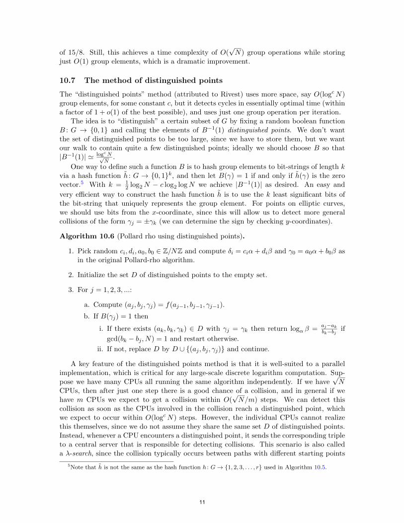
of 15/8. Still, this achieves a time complexity of O(√N) group operations while storing

just O(1) group elements, which is a dramatic improvement.

10.7 The method of distinguished points

The “distinguished points” method (attributed to Rivest) uses more space, say O(logcN)group elements, for some constant c, but it detects cycles in essentially optimal time (withina factor of 1 + o(1) of the best possible), and uses just one group operation per iteration.

The idea is to “distinguish” a certain subset of G by fixing a random boolean functionB : G → 0, 1 and calling the elements of B−1(1) distinguished points. We don’t wantthe set of distinguished points to be too large, since we have to store them, but we wantour walk to contain quite a few distinguished points; ideally we should choose B so that|B−1(1)| ' logcN√ .

NOne way to define such a function B is to hash group elements to bit-strings of length k

˜via a hash function h : G5 1

→ ˜0, 1k, and then let B(γ) = 1 if and only if h(γ) is the zerovector. With k = log N − c log logN we achieve |B−1(1)2 2 2 | as desired. An easy and

˜very efficient way to construct the hash function h is to use the k least significant bits ofthe bit-string that uniquely represents the group element. For points on elliptic curves,we should use bits from the x-coordinate, since this will allow us to detect more generalcollisions of the form γj = ±γk (we can determine the sign by checking y-coordinates).

Algorithm 10.6 (Pollard rho using distinguished points).

1. Pick random ci, di, a0, b0 ∈ Z/NZ and compute δi = ciα+ diβ and γ0 = a0α+ b0β asin the original Pollard-rho algorithm.

2. Initialize the set D of distinguished points to the empty set.

3. For j = 1, 2, 3, ...:

a. Compute (aj , bj , γj) = f(aj 1, b ,− j−1 γj−1).

b. If B(γj) = 1 then

i. If there exists (ak, bk, γk) ∈a a

D with γ = γk then return logα β = jj

− k ifbk−bjgcd(bk − bj , N) = 1 and restart otherwise.

ii. If not, replace D by D ∪ (aj , bj , γj) and continue.

A key feature of the distinguished points method is that it is well-suited to a parallelimplementation, which is critical for any large-scale discrete logarithm computation. Sup-pose we have many CPUs all running the same algorithm independently. If we have

√N

CPUs, then after just one step there is a good chancehave m CPUs we expect to get a collision within O(

√of a collision, and in general if weN/m) steps. We can detect this

collision as soon as the CPUs involved in the collision reach a distinguished point, whichwe expect to occur within O(logcN) steps. However, the individual CPUs cannot realizethis themselves, since we do not assume they share the same set D of distinguished points.Instead, whenever a CPU encounters a distinguished point, it sends the corresponding tripleto a central server that is responsible for detecting collisions. This scenario is also calleda λ-search, since the collision typically occurs between paths with different starting points

5 ˜Note that h is not the same as the hash function h : G→ 1, 2, 3, . . . , r used in Algorithm 10.5.

11

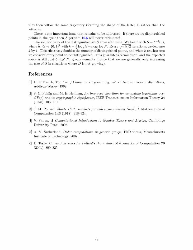
that then follow the same trajectory (forming the shape of the letter λ, rather than theletter ρ).

There is one important issue that remains to be addressed. If there are no distinguishedpoints in the cycle then Algorithm 10.6 will never terminate!

˜The solution is to let the distinguished set S grow with time. We begin with S = h−1(0),˜where h : G→ 0, 1k with k = 1

2 log2N−c log2 logN . Every√πN/2 iterations, we decrease

k by 1. This effectively doubles the number of distinguished points, and when k reaches zerowe consider every point to be distinguished. This guarantees termination, and the expectedspace is still just O(logcN) group elements (notice that we are generally only increasingthe size of S in situations where D is not growing).

References

[1] D. E. Knuth, The Art of Computer Programming, vol. II: Semi-numerical Algorithms,Addison-Wesley, 1969.

[2] S. C. Pohlig and M. E. Hellman, An improved algorithm for computing logarithms overGF (p) and its cryptographic significance, IEEE Transactions on Information Theory 24(1978), 106–110.

[3] J. M. Pollard, Monte Carlo methods for index computation (mod p), Mathematics ofComputation 143 (1978), 918–924.

[4] V. Shoup, A Computational Introduction to Number Theory and Algebra, CambridgeUniversity Press, 2005.

[5] A. V. Sutherland, Order computations in generic groups, PhD thesis, MassachusettsInstitute of Technology, 2007.

[6] E. Teske, On random walks for Pollard’s rho method, Mathematics of Computation 70(2001), 809–825.

12

MIT OpenCourseWarehttp://ocw.mit.edu

18.783 Elliptic CurvesSpring 2013

For information about citing these materials or our Terms of Use, visit: http://ocw.mit.edu/terms.