Copyright © 2016 Cengage Learning. All rights reserved.

15.1 Double Integrals overRectangles

2

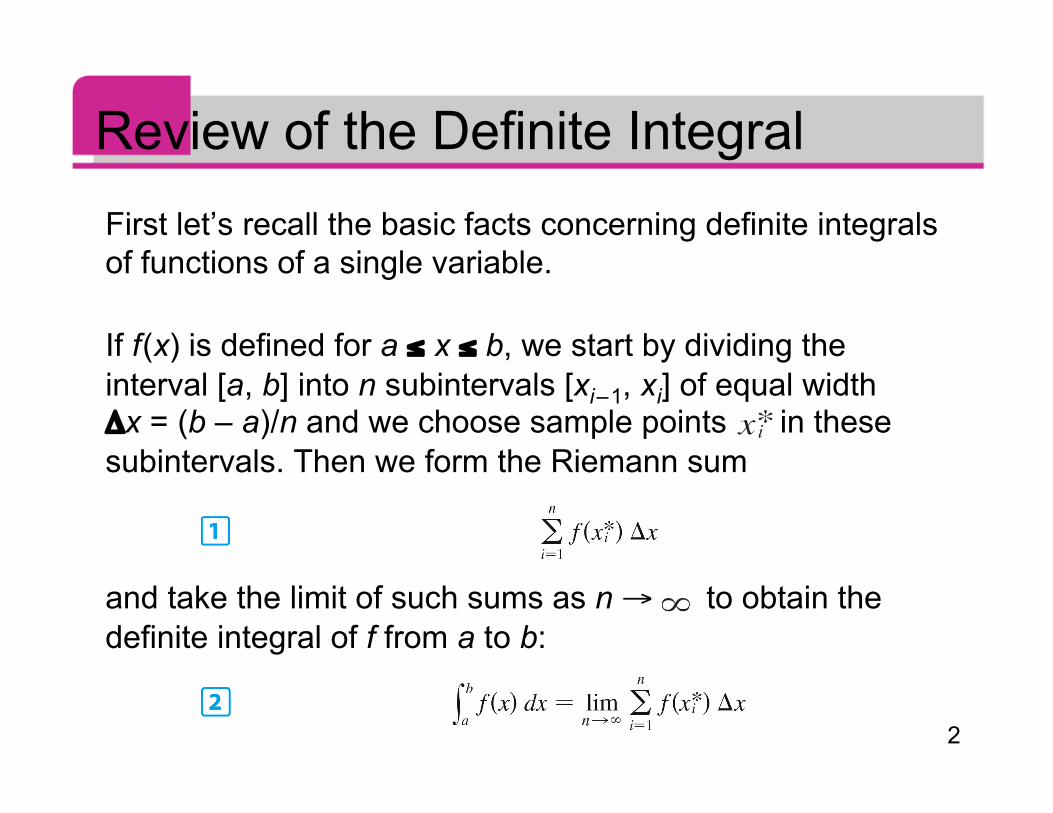
Review of the Definite IntegralFirst let’s recall the basic facts concerning definite integralsof functions of a single variable.

If f (x) is defined for a ≤ x ≤ b, we start by dividing theinterval [a, b] into n subintervals [xi – 1, xi] of equal widthΔx = (b – a)/n and we choose sample points in thesesubintervals. Then we form the Riemann sum

and take the limit of such sums as n → to obtain thedefinite integral of f from a to b:

3

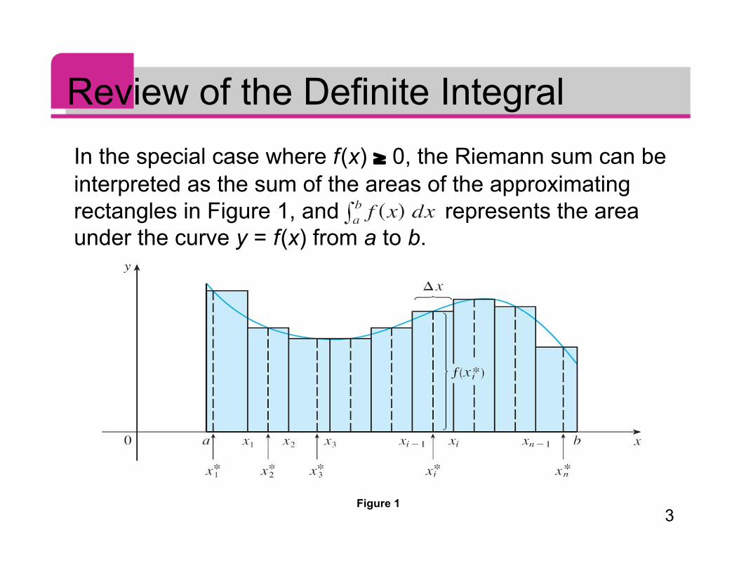
Review of the Definite IntegralIn the special case where f (x) ≥ 0, the Riemann sum can beinterpreted as the sum of the areas of the approximatingrectangles in Figure 1, and represents the areaunder the curve y = f (x) from a to b.

Figure 1

4

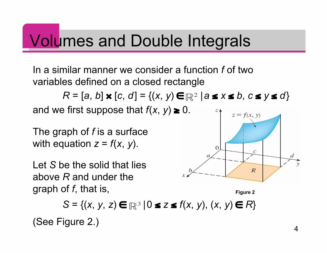
In a similar manner we consider a function f of twovariables defined on a closed rectangle

R = [a, b] × [c, d ] = {(x, y) ∈ | a ≤ x ≤ b, c ≤ y ≤ d }and we first suppose that f (x, y) ≥ 0.

The graph of f is a surfacewith equation z = f (x, y).

Let S be the solid that liesabove R and under thegraph of f, that is,

S = {(x, y, z) ∈ | 0 ≤ z ≤ f (x, y), (x, y) ∈ R}

(See Figure 2.)

Volumes and Double Integrals

Figure 2

5

Volumes and Double IntegralsOur goal is to find the volume of S.

The first step is to divide the rectangle R intosubrectangles.

We accomplish this by dividing the interval [a, b] into msubintervals [xi – 1, xi] of equal width Δx = (b – a)/m anddividing [c, d ] into n subintervals [yj – 1, yj] of equal widthΔy = (d – c)/n.

6

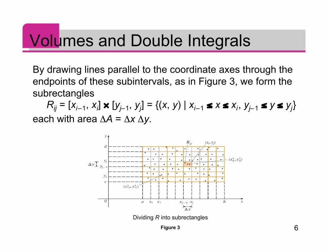
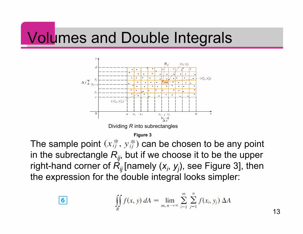
Volumes and Double IntegralsBy drawing lines parallel to the coordinate axes through theendpoints of these subintervals, as in Figure 3, we form thesubrectangles Rij = [xi – 1, xi] × [yj– 1, yj] = {(x, y) | xi – 1 ≤ x ≤ xi , yj– 1 ≤ y ≤ yj }each with area ΔA = Δx Δy.

Figure 3

Dividing R into subrectangles

7

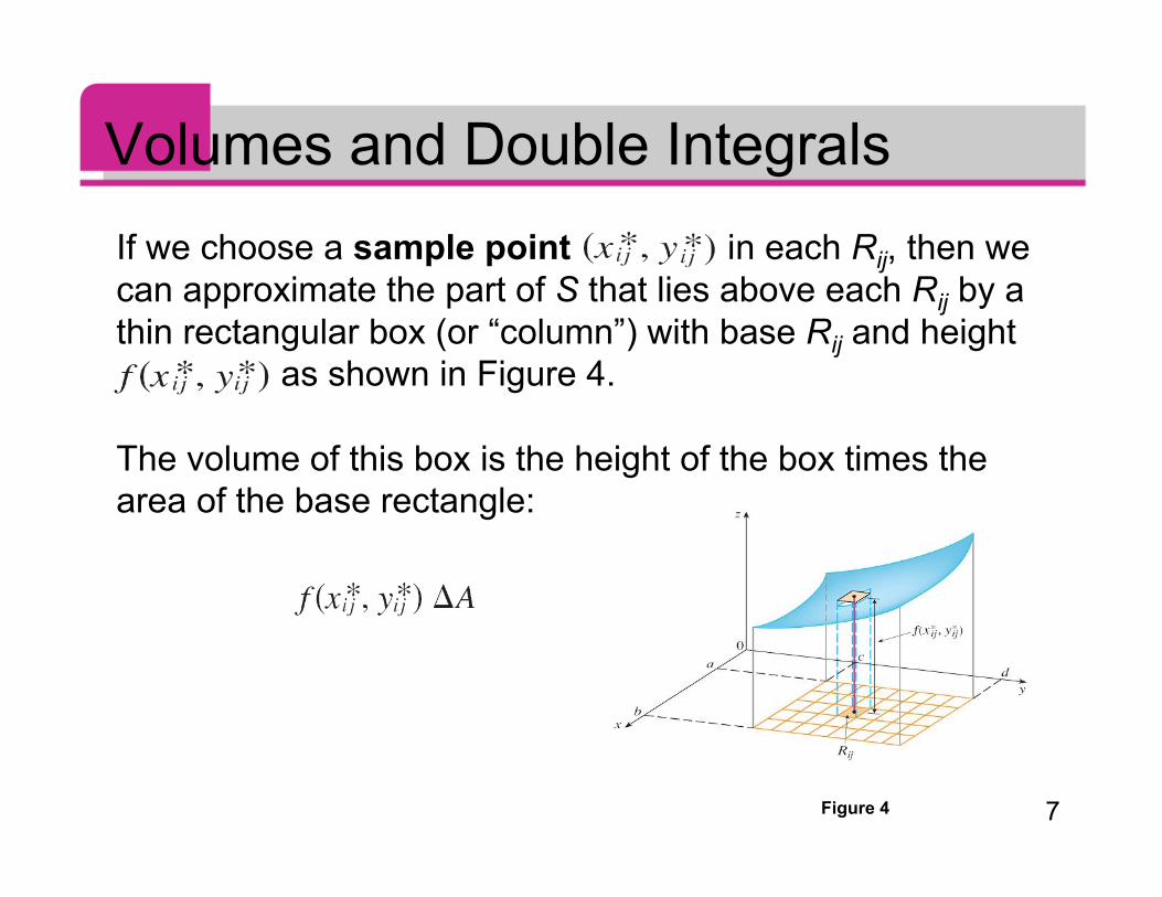
Volumes and Double IntegralsIf we choose a sample point in each Rij, then wecan approximate the part of S that lies above each Rij by athin rectangular box (or “column”) with base Rij and height

as shown in Figure 4.

The volume of this box is the height of the box times thearea of the base rectangle:

Figure 4

8

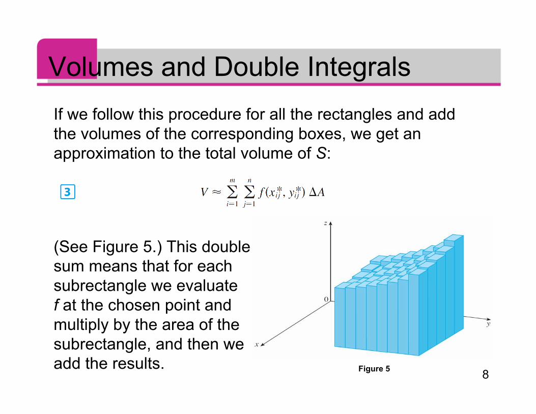
Volumes and Double IntegralsIf we follow this procedure for all the rectangles and addthe volumes of the corresponding boxes, we get anapproximation to the total volume of S:

(See Figure 5.) This doublesum means that for eachsubrectangle we evaluatef at the chosen point andmultiply by the area of thesubrectangle, and then weadd the results. Figure 5

9

Volumes and Double IntegralsOur intuition tells us that the approximation given in (3)becomes better as m and n become larger and so wewould expect that

We use the expression in Equation 4 to define the volumeof the solid S that lies under the graph of f and above therectangle R.

10

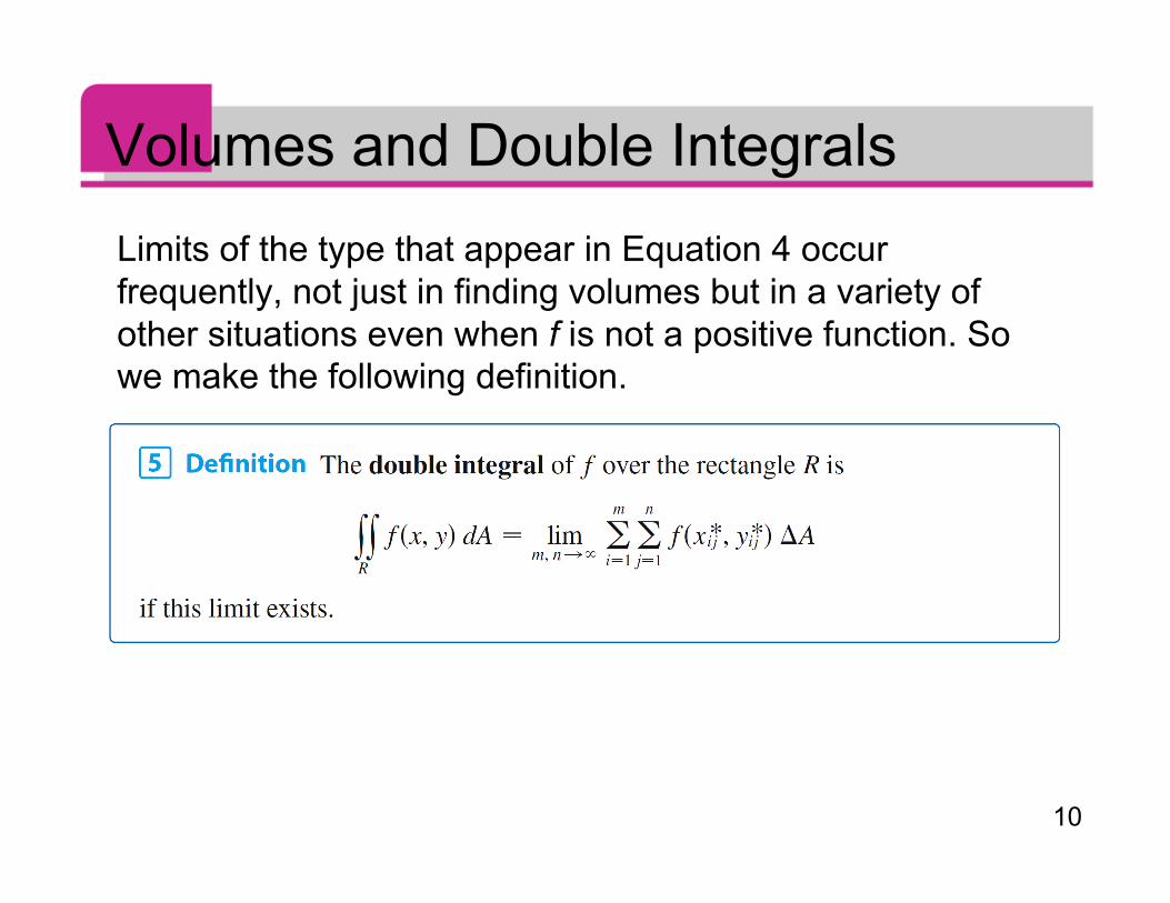
Volumes and Double IntegralsLimits of the type that appear in Equation 4 occurfrequently, not just in finding volumes but in a variety ofother situations even when f is not a positive function. Sowe make the following definition.

11

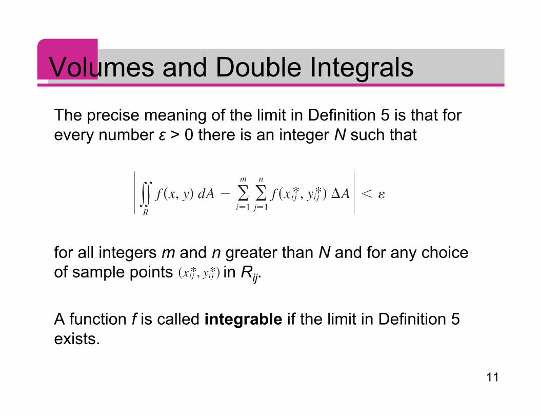
Volumes and Double IntegralsThe precise meaning of the limit in Definition 5 is that forevery number ε > 0 there is an integer N such that

for all integers m and n greater than N and for any choiceof sample points in Rij.

A function f is called integrable if the limit in Definition 5exists.

12

Volumes and Double IntegralsIt is shown in courses on advanced calculus that allcontinuous functions are integrable. In fact, the doubleintegral of f exists provided that f is “not too discontinuous.”

In particular, if f is bounded on R, [that is, there is aconstant M such that | f (x, y) | ≤ M for all (x, y) in R], and f iscontinuous there, except on a finite number of smoothcurves, then f is integrable over R.

13

Volumes and Double Integrals

The sample point can be chosen to be any pointin the subrectangle Rij, but if we choose it to be the upperright-hand corner of Rij [namely (xi, yj), see Figure 3], thenthe expression for the double integral looks simpler:

Figure 3

Dividing R into subrectangles

14

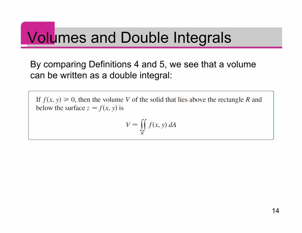
Volumes and Double IntegralsBy comparing Definitions 4 and 5, we see that a volumecan be written as a double integral:

15

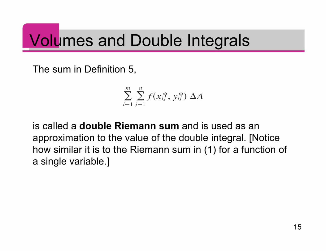
Volumes and Double IntegralsThe sum in Definition 5,

is called a double Riemann sum and is used as anapproximation to the value of the double integral. [Noticehow similar it is to the Riemann sum in (1) for a function ofa single variable.]

16

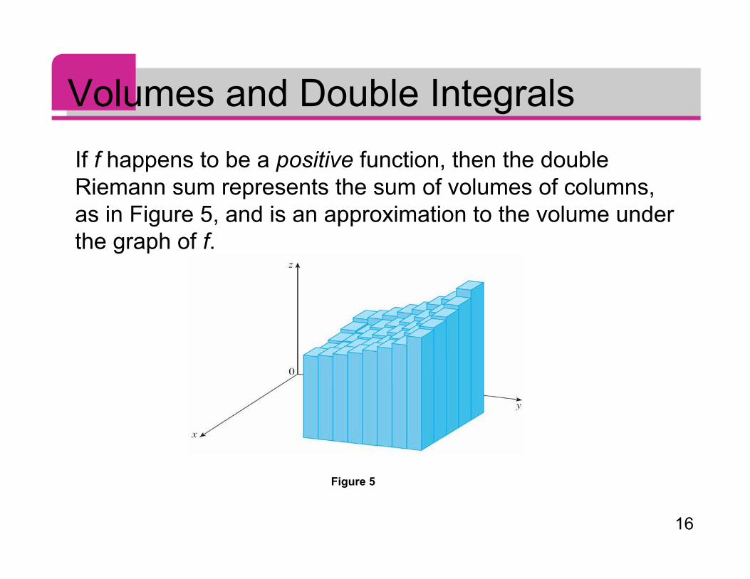
Volumes and Double IntegralsIf f happens to be a positive function, then the doubleRiemann sum represents the sum of volumes of columns,as in Figure 5, and is an approximation to the volume underthe graph of f.

Figure 5

17

Example 1Estimate the volume of the solid that lies above the squareR = [0, 2] × [0, 2] and below the elliptic paraboloidz = 16 – x2 – 2y2. Divide R into four equal squares andchoose the sample point to be the upper right corner ofeach square Rij. Sketch the solid and the approximatingrectangular boxes.

18

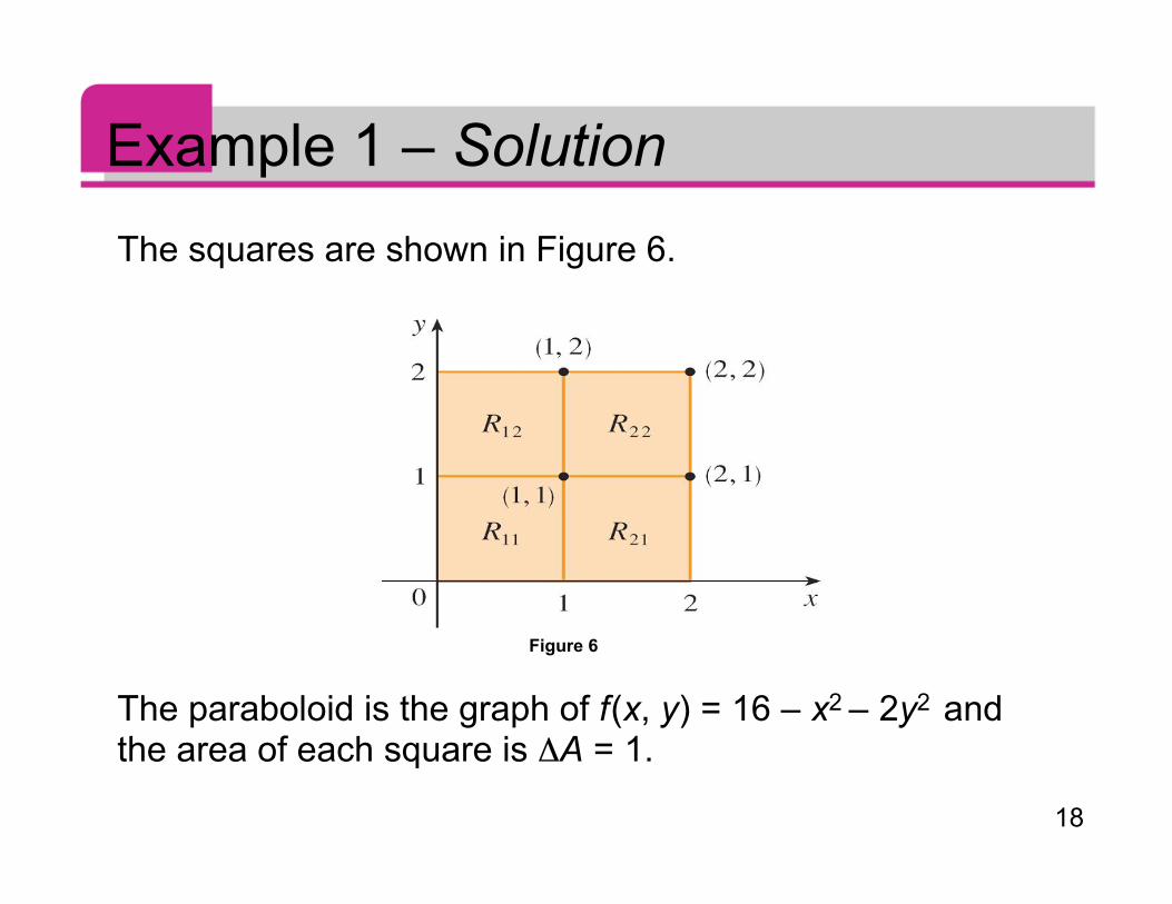
Example 1 – SolutionThe squares are shown in Figure 6.

The paraboloid is the graph of f (x, y) = 16 – x2 – 2y2 andthe area of each square is ΔA = 1.

Figure 6

19

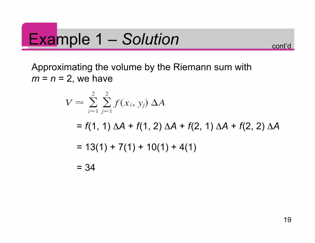
Example 1 – SolutionApproximating the volume by the Riemann sum withm = n = 2, we have

= f (1, 1) ΔA + f (1, 2) ΔA + f (2, 1) ΔA + f (2, 2) ΔA

= 13(1) + 7(1) + 10(1) + 4(1)

= 34

cont’d

20

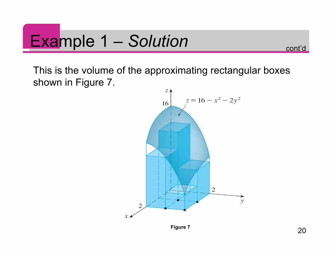
Example 1 – SolutionThis is the volume of the approximating rectangular boxesshown in Figure 7.

Figure 7

cont’d

21

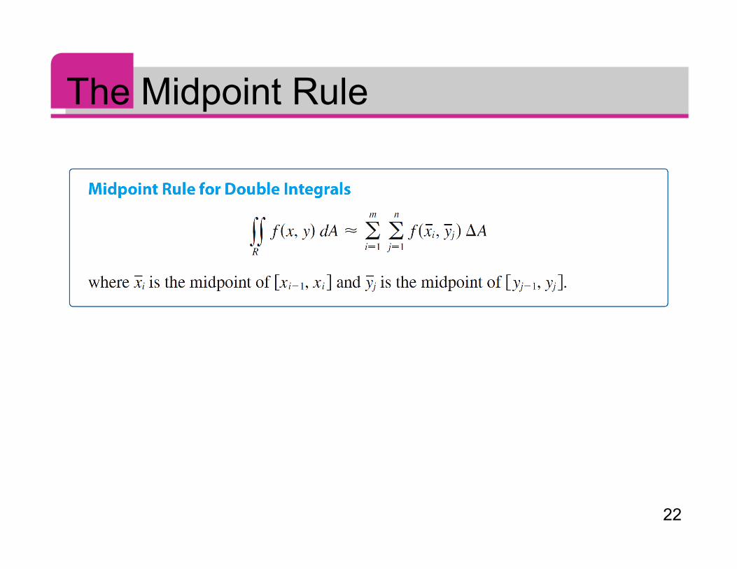
The Midpoint RuleThe methods that we used for approximating singleintegrals (the Midpoint Rule, the Trapezoidal Rule,Simpson’s Rule) all have counterparts for double integrals.Here we consider only the Midpoint Rule for doubleintegrals.

This means that we use a double Riemann sum toapproximate the double integral, where the sample point

in Rij is chosen to be the center of Rij. Inother words, is the midpoint of [xi – 1, xi] and is themidpoint of [yj – 1, yj].

22

The Midpoint Rule

23

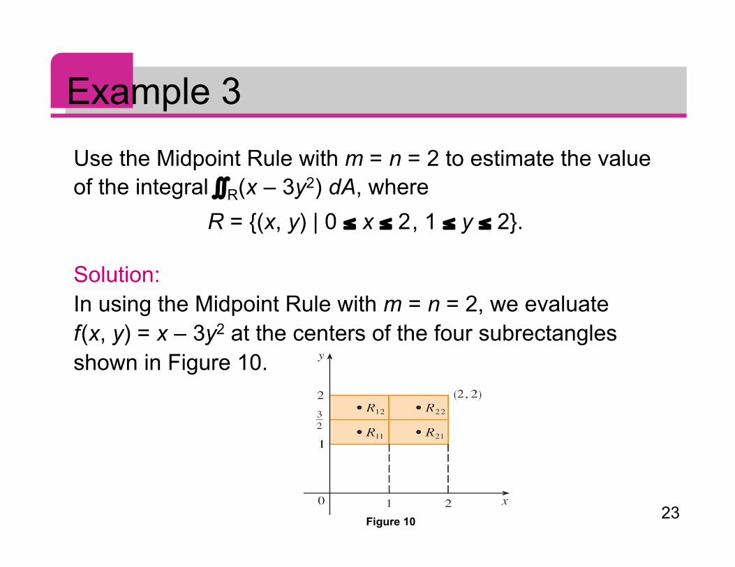
Example 3

Use the Midpoint Rule with m = n = 2 to estimate the valueof the integral ∫∫R(x – 3y2) dA, where

R = {(x, y) | 0 ≤ x ≤ 2 , 1 ≤ y ≤ 2}.

Solution:In using the Midpoint Rule with m = n = 2, we evaluatef (x, y) = x – 3y2 at the centers of the four subrectanglesshown in Figure 10.

Figure 10

24

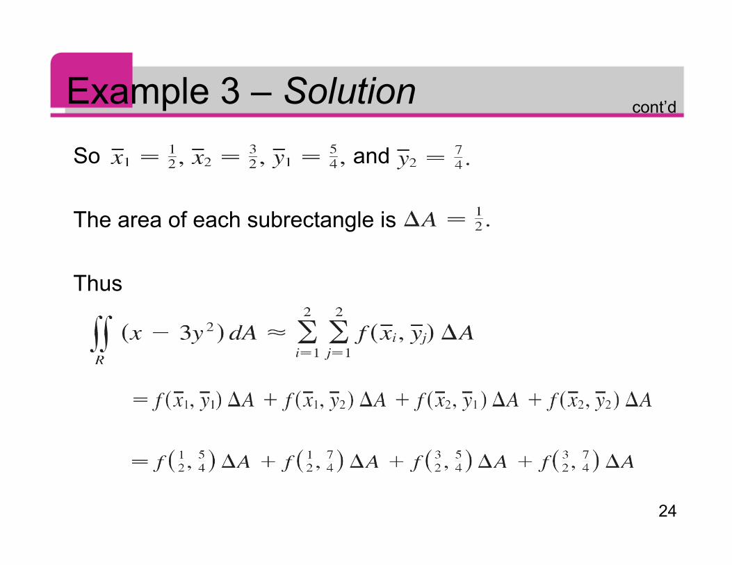
Example 3 – SolutionSo and

The area of each subrectangle is

Thus

cont’d

25

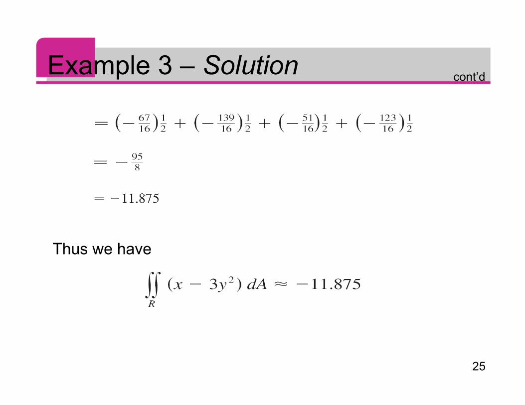
Example 3 – Solution

Thus we have

cont’d

26

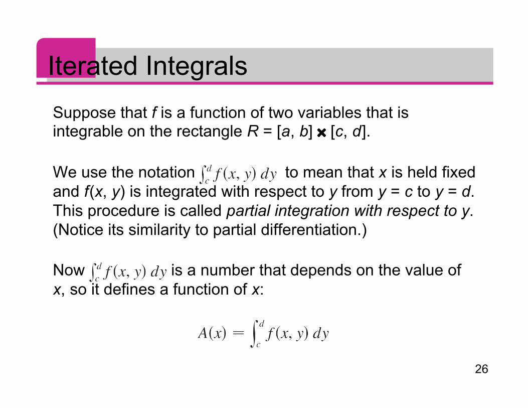
Iterated IntegralsSuppose that f is a function of two variables that isintegrable on the rectangle R = [a, b] × [c, d ].

We use the notation to mean that x is held fixedand f (x, y) is integrated with respect to y from y = c to y = d.This procedure is called partial integration with respect to y.(Notice its similarity to partial differentiation.)

Now is a number that depends on the value ofx, so it defines a function of x:

27

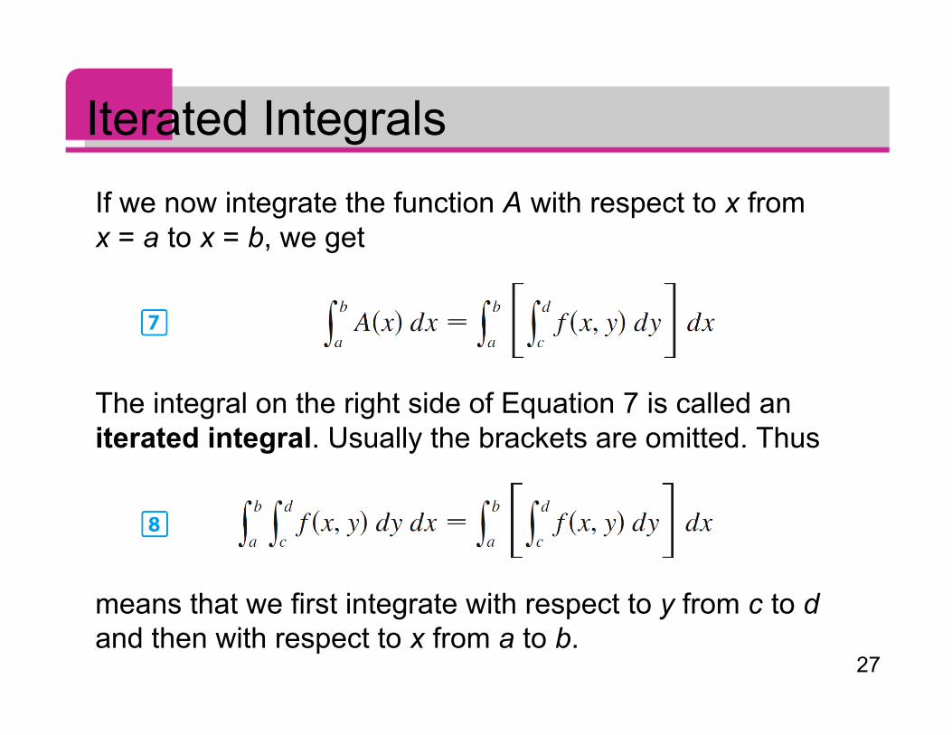
Iterated IntegralsIf we now integrate the function A with respect to x fromx = a to x = b, we get

The integral on the right side of Equation 7 is called aniterated integral. Usually the brackets are omitted. Thus

means that we first integrate with respect to y from c to dand then with respect to x from a to b.

28

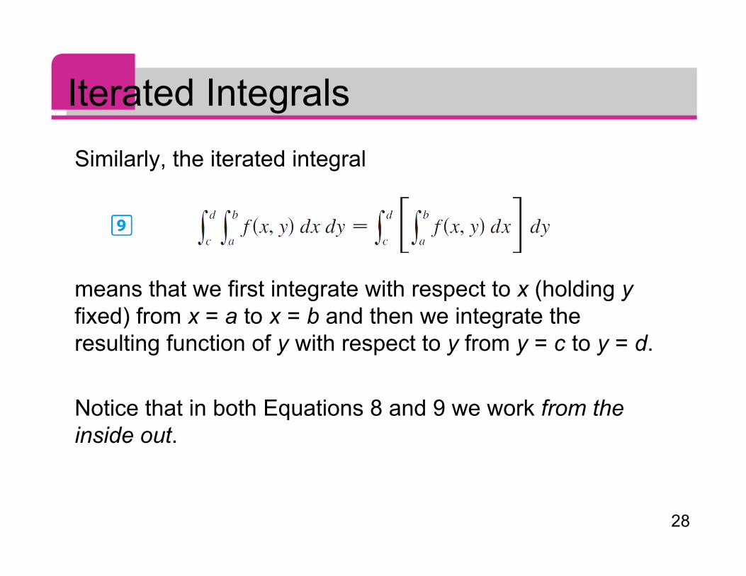
Iterated IntegralsSimilarly, the iterated integral

means that we first integrate with respect to x (holding yfixed) from x = a to x = b and then we integrate theresulting function of y with respect to y from y = c to y = d.

Notice that in both Equations 8 and 9 we work from theinside out.

29

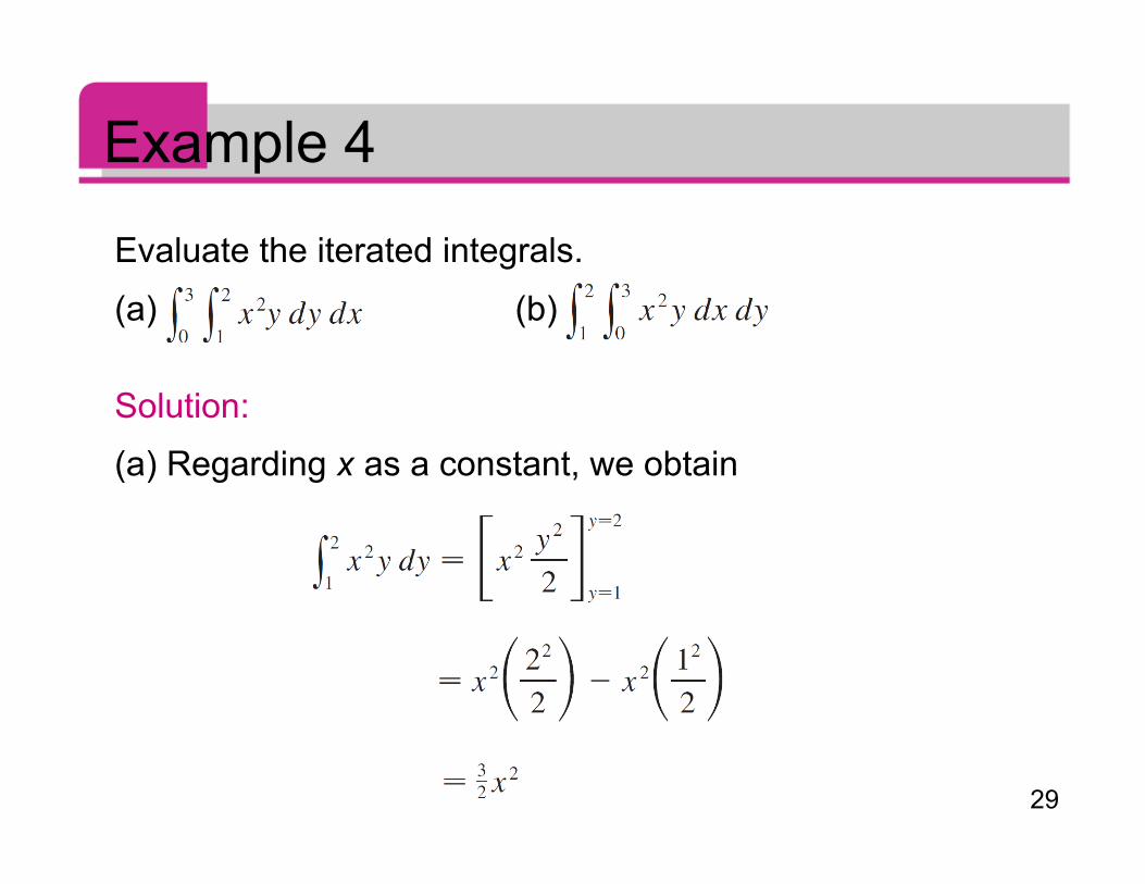
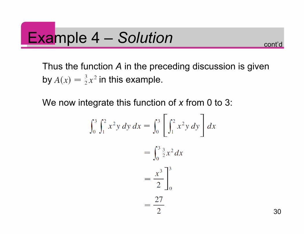
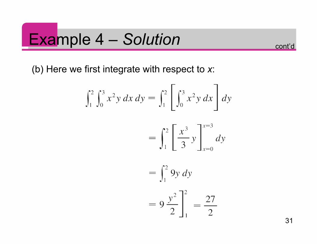
Example 4

Evaluate the iterated integrals.

(a) (b)

Solution:

(a) Regarding x as a constant, we obtain

30

Example 4 – Solution

Thus the function A in the preceding discussion is givenby in this example.

We now integrate this function of x from 0 to 3:

cont’d

31

Example 4 – Solution

(b) Here we first integrate with respect to x:

cont’d

32

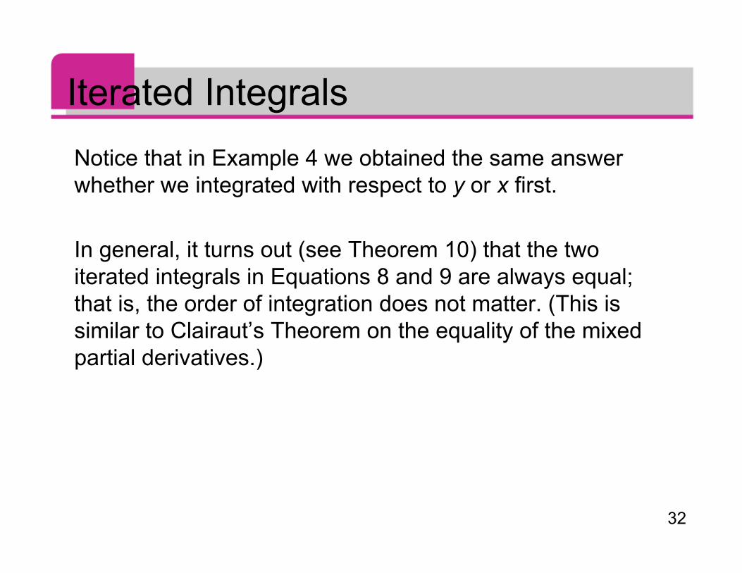
Iterated IntegralsNotice that in Example 4 we obtained the same answerwhether we integrated with respect to y or x first.

In general, it turns out (see Theorem 10) that the twoiterated integrals in Equations 8 and 9 are always equal;that is, the order of integration does not matter. (This issimilar to Clairaut’s Theorem on the equality of the mixedpartial derivatives.)

33

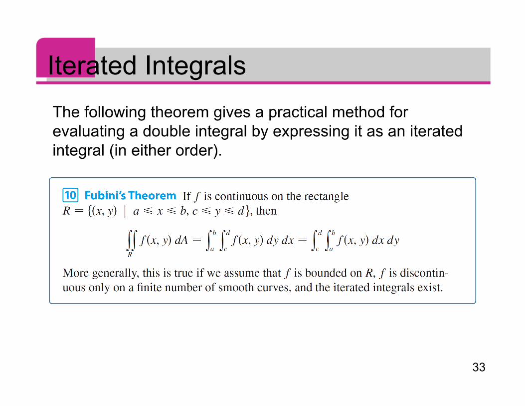
Iterated IntegralsThe following theorem gives a practical method forevaluating a double integral by expressing it as an iteratedintegral (in either order).

34

Iterated IntegralsIn the special case where f (x, y) can be factored as theproduct of a function of x only and a function of y only, thedouble integral of f can be written in a particularly simpleform.

To be specific, suppose that f (x, y) = g (x)h (y) andR = [a, b] × [c, d].

Then Fubini’s Theorem gives

35

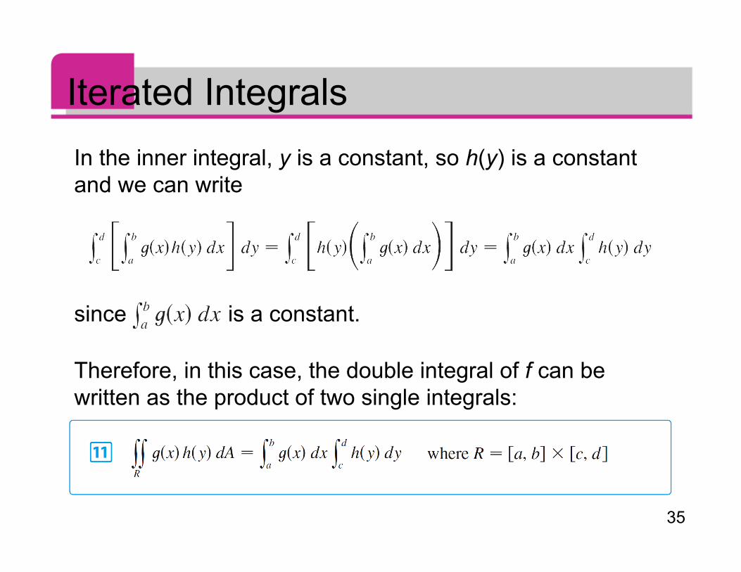
Iterated IntegralsIn the inner integral, y is a constant, so h(y) is a constantand we can write

since is a constant.

Therefore, in this case, the double integral of f can bewritten as the product of two single integrals:

36

Average ValueWe know that the average value of a function f of onevariable defined on an interval [a, b] is

In a similar fashion we define the average value of afunction f of two variables defined on a rectangle R to be

where A(R) is the area of R.

37

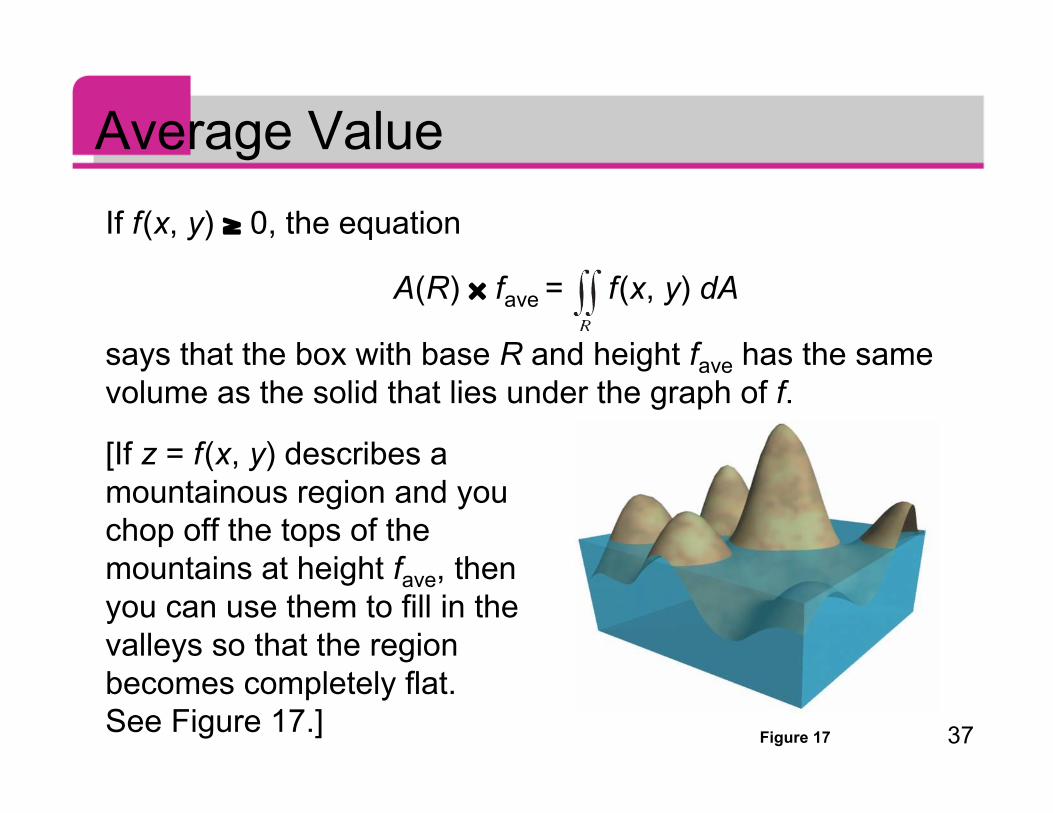
Average ValueIf f (x, y) ≥ 0, the equation

A(R) × fave = f (x, y) dA

says that the box with base R and height fave has the samevolume as the solid that lies under the graph of f.

[If z = f (x, y) describes amountainous region and youchop off the tops of themountains at height fave, thenyou can use them to fill in thevalleys so that the regionbecomes completely flat.See Figure 17.] Figure 17

38

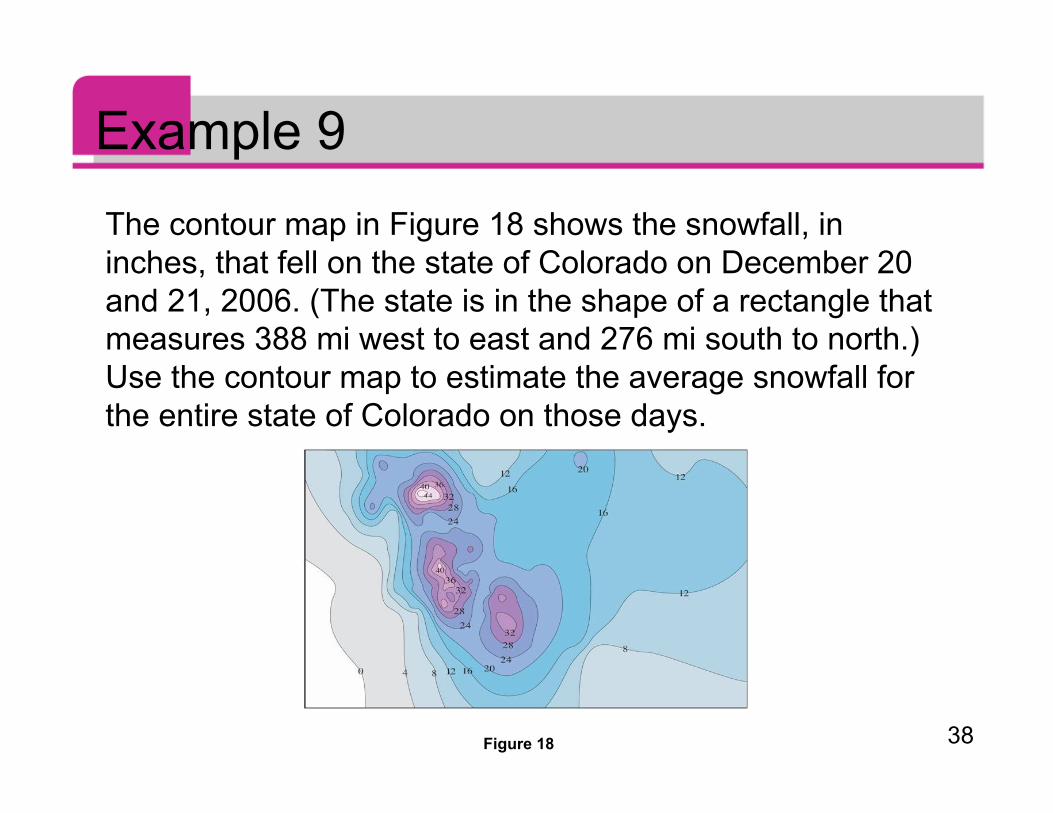
Example 9The contour map in Figure 18 shows the snowfall, ininches, that fell on the state of Colorado on December 20and 21, 2006. (The state is in the shape of a rectangle thatmeasures 388 mi west to east and 276 mi south to north.)Use the contour map to estimate the average snowfall forthe entire state of Colorado on those days.

Figure 18

39

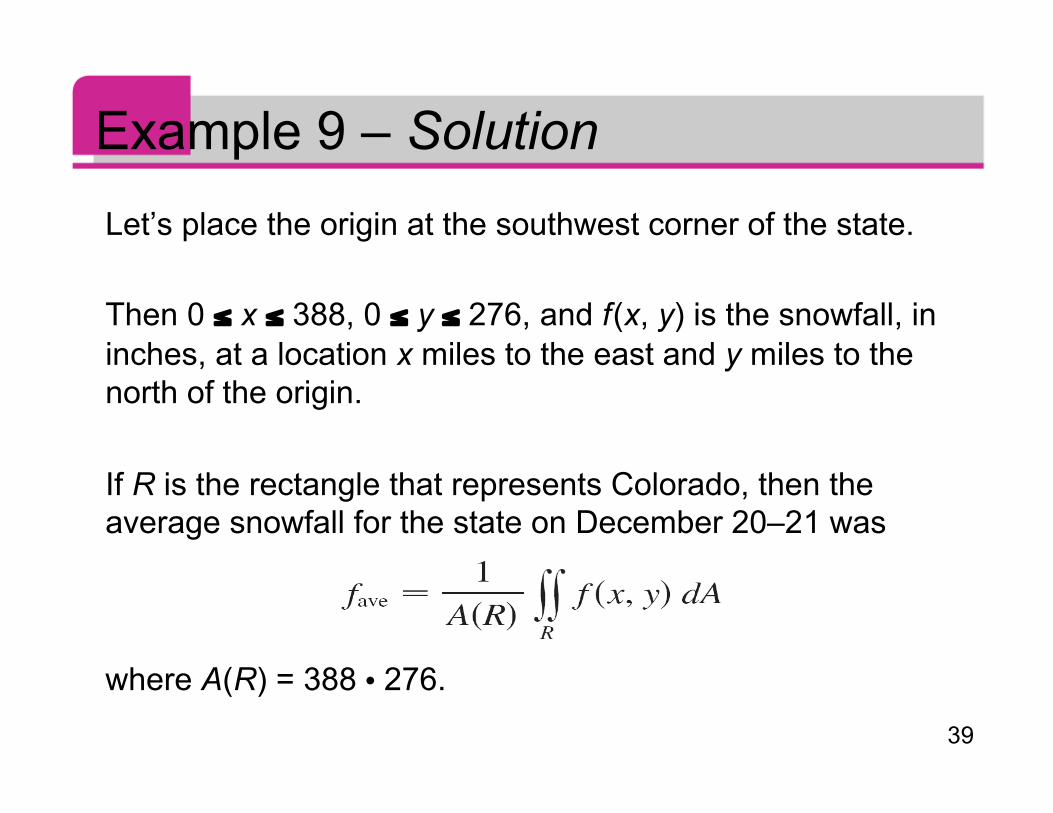
Example 9 – SolutionLet’s place the origin at the southwest corner of the state.

Then 0 ≤ x ≤ 388, 0 ≤ y ≤ 276, and f (x, y) is the snowfall, ininches, at a location x miles to the east and y miles to thenorth of the origin.

If R is the rectangle that represents Colorado, then theaverage snowfall for the state on December 20–21 was

where A(R) = 388 276.

40

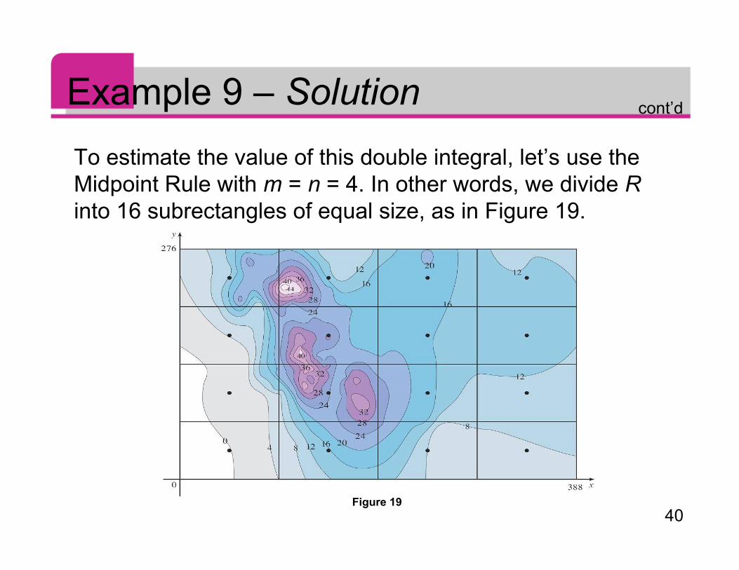
Example 9 – SolutionTo estimate the value of this double integral, let’s use theMidpoint Rule with m = n = 4. In other words, we divide Rinto 16 subrectangles of equal size, as in Figure 19.

Figure 19

cont’d

41

Example 9 – SolutionThe area of each subrectangle is

Using the contour map to estimate the value of f at the centerof each subrectangle, we get

≈ ΔA[0 + 15 + 8 + 7 + 2 + 25 + 18.5 + 11 + 4.5 + 28 + 17 + 13.5 + 12 + 15 + 17.5 + 13]

= (6693)(207)

= 6693 mi2

cont’d

42

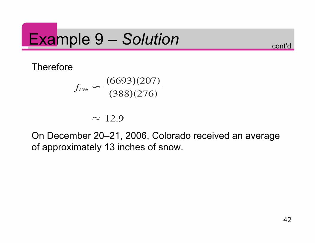
Example 9 – SolutionTherefore

On December 20–21, 2006, Colorado received an averageof approximately 13 inches of snow.

cont’d