15 Forecasting Time Series

15.1 Forecasting Stationary Time Series

We investigate the problem of predicting the values Xn+h, h > 0, of a stationary timeseries with known mean µ and autocovariance function γ in terms of {Xn, . . . , X1}. Ourgoal is to find the linear combination of 1, Xn, Xn−1, . . . , X1, that forecasts Xn+h withminimum mean squared error. The best linear predictor will be denoted by PnXn+h andclearly has the form

PnXn+h = a0 + a1Xn + . . .+ anX1.

It remains to determine the coefficients a0, . . . , an, by finding the values that minimize

S(a0, . . . , an) = E(Xn+h − a0 − a1Xn − . . .− anX1)2.

Since S is a quadratic function of a0, . . . , an and is bounded below by zero, it is clearthat there is at least one value of (a0, . . . , an) that minimizes S and that the minimumsatisfies

∂S(a0, . . . , an)

∂aj= 0, j = 0, . . . , n.

Evaluation of the derivatives gives the equivalent equations

E

[Xn+h − a0 −

n∑

i=1

aiXn+1−i

]= 0, (15.1)

E

[(Xn+h − a0 −

n∑

i=1

aiXn+1−i

)Xn+1−j

]= 0, j = 1, . . . , n. (15.2)

These equations can be written as

a0 = µ

(1−

n∑

i=1

ai

), (15.3)

Γnan = γn(h), (15.4)

where an = (a1, . . . , an)′, Γn := [γ(i− j)]ni,j=1 and γn(h) := (γ(h), . . . , γ(h+ n− 1))′.

Proposition 15.1.1. The the best linear predictor PnXn+h is

PnXn+h = µ+n∑

i=1

ai(Xn+1−i − µ), (15.5)

where an satisfies (15.4). From (15.5) the expected value of the prediction error Xn+h−PnXn+h is zero, and the mean square prediction error is therefore

E(Xn+h − PnXn+h)2 = γ(0)− an

′γn(h),

where an = (a1, . . . , an)′ and γn(h) := (γ(h), . . . , γ(h+ n− 1))′ .

15-1

Remark. If {Yt} is a stationary time series with mean µ and if {Xt} is the zero-meanseries defined by Xt = Yt − µ, then PnYn+h = µ + PnXn+h. So from now on, we canrestrict attention to zero-mean stationary time series.

Example. Consider the time series

Xt = φXt−1 + Zt, t = 0,±1, . . . ,

where |φ| < 1 and Zt ∼ WN(0, σ2). The best linear predictor of Xn+1 in terms of{1, Xn, . . . , X1} is

PnXn+1 = a′nXn,

where Xn = (Xn, . . . , X1)′ and

1 φ . . . φn−1

φ 1 . . . φn−2

......

. . ....

φn−1 φn−2 . . . 1

a1

a2...

an

=

φ

φ2

...

φn

.

A solution is clearlyan = (φ, 0, . . . , 0)′,

and hence the best linear predictor of Xn+1 in terms of {X1, . . . , Xn} is

PnXn+1 = a′nXn = φXn,

with mean squared error

E(Xn+1 − PnXn+1)2 = γ(0)− a′nγn(1) =

σ2

1− φ2− φγ(1) = σ2.

Remark. If {Xt} is a zero-mean stationary series with autocovariance function γ(·), thenin principle determining the best linear predictor PnXn+h in terms of {Xn, . . . , X1} ispossible. However, the direct approach requires the determination of a solution of asystem of n linear equations, which for large n may be difficult and time-consuming.Therefore it would be helpful if the one-step predictor PnXn+1 based on the n previousobservations could be used to simplify the calculation of Pn+1Xn+2, the one-step predic-tor based on n+1 previous observations. Prediction algorithms that utilize this idea aresaid to be recursive. The algorithms to be discussed in this chapter allow us to computebest predictors without having to perform any matrix inversions.

Remark. There are two important recursive prediction algorithms:

� Durbin-Levinson algorithm: Section 15.1.1 and Brockwell and Davis (2002) pp. 69-71.

� Innovations algorithm: Section 15.1.2, Section 16.1.3, Brockwell and Davis (2002)pp. 71-75 and pp. 150-156.

15-2

15.1.1 Durbin-Levinson Algorithm

From Proposition 15.1.1 we know that if the matrix Γn is nonsingular, then

PnXn+1 = φ′nXn = φn1Xn + . . .+ φnnX1, (15.6)

whereφn = Γ−1n γn, γn = (γ(1), . . . , γ(n))′

and the corresponding mean squared error is

νn := E(Xn+1 − PnXn+1)2 = γ(0)− φn

′γn.

A useful sufficient condition for nonsingularity of all the autocovariance matrices Γ1,Γ2, . . .is γ(0) > 0 and γ(h) → 0 as h → ∞. The coefficients φn1, . . . , φnn can be computedrecursively with the Durbin-Levinson algorithm (see Figure 15.1).

Figure 15.1: Algorithm for estimating the parameters φn = (φn1, . . . , φnn) in a pureautoregressive model. Source: Brockwell and Davis (2002), p. 70.

15.1.2 Innovations Algorithm

The recursive algorithm to be discussed in this section is applicable to all series withfinite second moments, regardless of whether they are stationary or not. Its application,however, can be simplified in certain special cases.

15-3

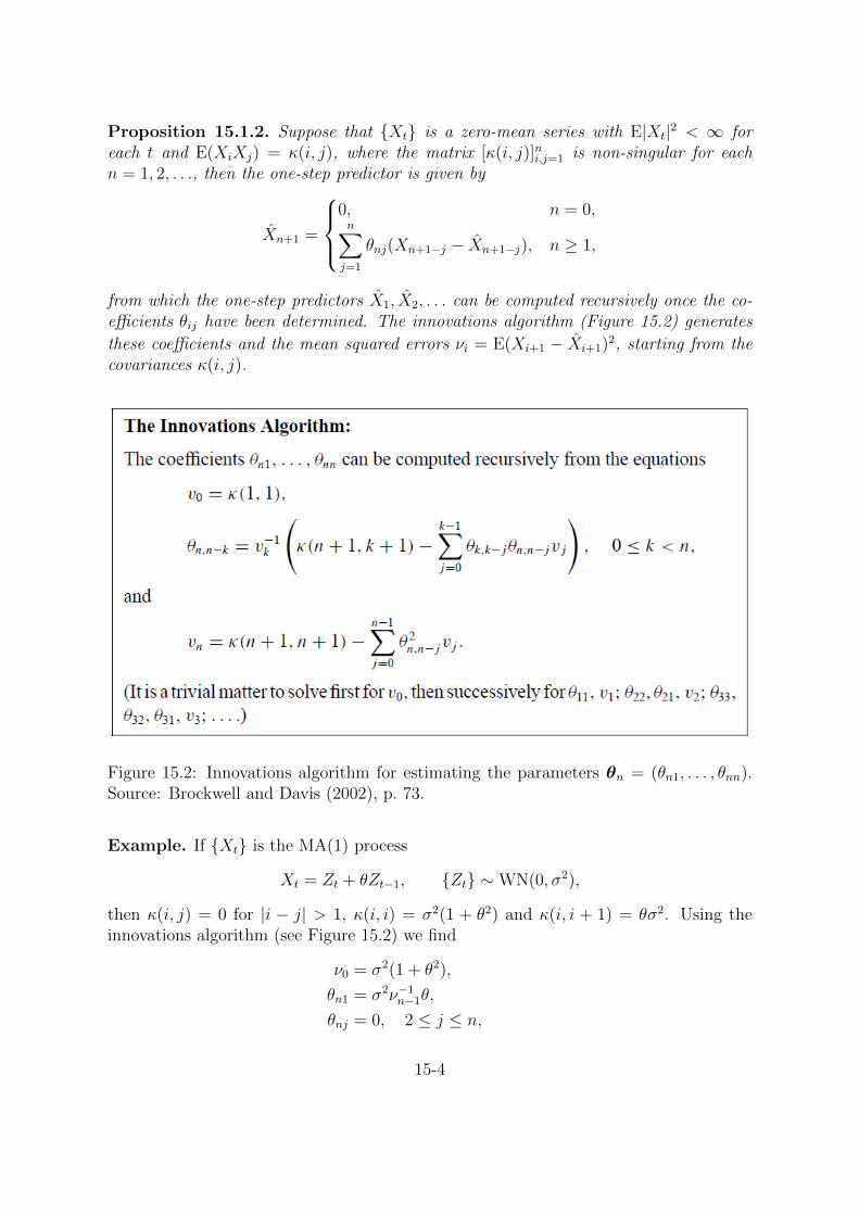
Proposition 15.1.2. Suppose that {Xt} is a zero-mean series with E|Xt|2 < ∞ foreach t and E(XiXj) = κ(i, j), where the matrix [κ(i, j)]ni,j=1 is non-singular for eachn = 1, 2, . . ., then the one-step predictor is given by

Xn+1 =

0, n = 0,n∑

j=1

θnj(Xn+1−j − Xn+1−j), n ≥ 1,

from which the one-step predictors X1, X2, . . . can be computed recursively once the co-efficients θij have been determined. The innovations algorithm (Figure 15.2) generates

these coefficients and the mean squared errors νi = E(Xi+1 − Xi+1)2, starting from the

covariances κ(i, j).

Figure 15.2: Innovations algorithm for estimating the parameters θn = (θn1, . . . , θnn).Source: Brockwell and Davis (2002), p. 73.

Example. If {Xt} is the MA(1) process

Xt = Zt + θZt−1, {Zt} ∼WN(0, σ2),

then κ(i, j) = 0 for |i − j| > 1, κ(i, i) = σ2(1 + θ2) and κ(i, i + 1) = θσ2. Using theinnovations algorithm (see Figure 15.2) we find

ν0 = σ2(1 + θ2),

θn1 = σ2ν−1n−1θ,

θnj = 0, 2 ≤ j ≤ n,

15-4

and

νn = σ2[1 + θ2 − ν−1n−1θ2σ2].

If we define rn = νn/σ2, then we can write

Xn+1 =θ(Xn − Xn)

rn−1,

where r0 = 1 + θ2 and rn+1 = 1 + θ2 − θ2/rn.

15.2 Forecasting ARMA Processes

The innovations algorithm is a recursive method for forecasting second-order zero-meanprocesses that are not necessarily stationary. Proposition 15.1.2 can of course be applieddirectly to the prediction of the causal ARMA process,

φ(B)Xt = θ(B)Zt, {Zt} ∼WN(0, σ2).

However a drastic simplification in the calculations can be achieved, if, instead ofapplying Proposition 15.1.2 to {Xt}, we apply it to the transformed process

Wt =

{σ−1Xt, t = 1, . . . ,m,

σ−1φ(B)Xt, t > m,

where m = max(p, q).For notational convenience we define θ0 := 1, θj := 0 for j > q and assume that

p ≥ 1 and q ≥ 1. The autocovariances κ(i, j) = E(WiWj), i, j ≥ 1, are found from

κ(i, j) =

σ−2γX(i− j), 1 ≤ i, j ≤ m,

σ−2

[γX(i− j)−

p∑

r=1

φrγX(r − |i− j|)], min(i, j) ≤ m < max(i, j) ≤ 2m,

q∑

r=0

θrθr+|i−j|, min(i, j) > m,

0, otherwise.

(15.7)Applying the innovations algorithm to the process {Wt} and replacing (Wj− Wj) by

σ−1(Xj − Xj) we finally obtain

Xn+1 =

n∑

j=1

θnj(Xn+1−j − Xn+1−j), 1 ≤ n < m = max(p, q),

φ1Xn + . . .+ φpXn+1−p +

q∑

j=1

θnj(Xn+1−j − Xn+1−j), n ≥ m,

(15.8)

15-5

andE(Xn+1 − Xn+1)

2 = σ2 E(Wn+1 − Wn+1)2 = σ2rn,

where θnj and rn are found from the innovations algorithm (see Figure 15.2) with κ as

in (15.7). Equations (15.8) determine the one-step predictors X2, X3, . . . recursively.

Example. Prediction of ARMA(1, 1) processes. Let

Xt − φXt−1 = Zt + θZt−1, {Zt} ∼WN(0, σ2),

and |φ| < 1, then equations (15.8) reduce to the single equation

Xn+1 = φXn + θn1(Xn − Xn), n ≥ 1.

We know that

γX(0) = σ2 1 + 2θφ+ θ2

1− φ2.

Substituting in (15.7) then gives, for i, j ≥ 1,

κ(i, j) =

1 + 2θφ+ θ2

1− φ2, i = j = 1,

1 + θ2, i = j ≥ 2,

θ, |i− j| = 1, i ≥ 1,

0, otherwise.

With these values of κ(i, j), the recursions of the innovations algorithm reduce to

r0 =1 + 2θφ+ θ2

1− φ2, θn1 =

θ

rn−1, rn = 1 + θ2 − θ2

rn−1,

which can be solved quite explicitly.

15-6

16 Modeling with ARMAProcesses

The determination of an appropriate ARMA(p, q) model to represent an observed sta-tionary time series involves a number of interrelated problems. These include thechoice of p and q (order selection) and the estimation of the mean, the coefficients{φi, i = 1, . . . , p}, {θi, i = 1, . . . , q} and the white noise variance σ2. Final selection ofthe model depends on a variety of goodness of fit tests1, although it can be system-atized to a large degree by use of criteria such as minimization of the AICC statistic asdiscussed in Section 16.2.2.

When p and q are known, good estimators of φ and θ can be found by imaginingthe data to be observations of a stationary Gaussian time series and maximizing thelikelihood with respect to the p + q + 1 parameters φ1, . . . , φp, θ1, . . . , θq and σ2. Theestimators obtained by this procedure are known as maximum likelihood estimators(Section 16.2). The algorithm used to determine the maximum likelihood estimatorsrequires the specification of initial parameter values with which to begin the search.The closer the preliminary estimates are to the maximum likelihood estimates, the fasterthe search will generally be. To provide these initial values, a number of preliminaryestimation algorithms are available (Section 16.1).

Section 16.3 deals with goodness of fit tests for the chosen model and Chapter 15 withthe use of the fitted model for forecasting. In Section 16.2.2 we discuss the theoreticalbasis for some of the criteria used for order selection.

Remark. A good overview for determining an adequate ARMA model to a time series isgiven in Chapter 6 in Schlittgen and Streitberg (2001) (in German).

16.1 Preliminary Estimation

We shall consider different techniques for preliminary estimation of the parameters

φ = (φ1, . . . , φp), θ = (θ1, . . . , θq),

and σ2 from observations x1, . . . , xn of the causal ARMA(p, q) process defined by

φ(B)Xt = θ(B)Zt, {Zt} ∼WN(0, σ2). (16.1)

1. Pure autoregressive models:

� Yule-Walker procedure (Section 16.1.1)

� Burg’s procedure (Section 16.1.2)

1Goodness of fit tests are used to judge the adequacy of a given statistical model.

16-1

For pure autoregressive models Burg’s algorithm usually gives higher likelihoodsthan the Yule-Walker equations.

2. ARMA(p, q), p, q > 0:

� Innovations algorithm (Section 16.1.3 and Brockwell and Davis (2002), pp. 154–156)

� Hannan-Rissanen algorithm (Section 16.1.4)

For pure moving-average models the innovations algorithm frequently gives slightlyhigher likelihoods than than the Hannan-Rissanen algorithm. For mixed modelsthe Hannan-Rissanen algorithm is usually more successful in finding causal modelswhich are required for initialization of the likelihood maximization.

16.1.1 Yule-Walker Equations2

For a pure autoregressive model the causality assumption allows us to write Xt in theform

Xt =∞∑

j=0

ψjZt−j where ψ(z) =∞∑

j=0

ψjzj =

1

φ(z). (16.2)

Multiplying each side of (16.1) by Xt−j, j = 0, . . . , p, taking expectations, and using(16.2) to evaluate the right-hand side of the first equation, we obtain the Yule-Walkerequations

Γpφ = γp and σ2 = γ(0)− φ′γp,where Γp is the covariance matrix [γ(i− j)]pi,j=1 and γp = (γ(1), . . . , γ(p))′. These

equations can be used to determine γ(0), . . . , γ(p) from σ2 and φ.If we replace the covariances γ(j), j = 0, . . . , p by the corresponding sample covari-

ances γ(j), we obtain a set of equations for the so-called sample Yule-Walker estimatorsφ and σ2 of φ and σ2, namely,

Γpφ = γp (16.3)

and

σ2 = γ(0)− φ′γp (16.4)

whereΓp = [γ(i− j)]pi,j=1 and γp = (γ(1), . . . , γ(p))′ .

If γ(0) > 0, then Γm is nonsingular for everym = 1, 2, . . ., so we can rewrite equations(16.3) and (16.4) in the following form:

2Gibert Walker 1868-1958, George Udny Yule 1871-1951.

16-2

Definition 16.1.1 (Sample Yule-Walker equations).

φ =(φ1, . . . , φp

)′= R

−1p ρp

and

σ2 = γ(0)

(1− ρ′pR

−1p ρp

),

where

ρp = (ρ(1), . . . , ρ(p))′ = γp/γ(0) and Rp = Γp/γ(0).

Proposition 16.1.2 (Large-sample distribution of Yule-Walker equations). For a largesample from an AR(p) process

n1/2(φ− φ) ∼ Np(0, σ2Γ−1p ).

Order selection In practice we do not know the true order of the model generatingthe data. In fact, it will usually be the case that there is no true AR model, in whichcase our goal is simply to find one that represents the data optimally in some sense.Two useful techniques for selecting an appropriate AR model are given below:

� Some guidance in the choice of order is provided by a large-sample result whichstates that if {Xt} is A causal AR(p) process with {Zt} ∼ IID(0, σ2) and if we fit amodel with order m > p using the Yule-Walker equations, then the last component,φmm, of the vector φm is approximately normally distributed with mean 0 andvariance 1/n. Notice that φmm is exactly the sample partial autocorrelation at lagm.

Now, we already know that for an AR(p) process the partial autocorrelation func-tion φmm, m > p, are zero. Therefore, if an AR(p) model is appropriate for thedata, then the values φkk, k > p, should be compatible with observations fromN(0, 1/n). In particular, for k > p, φkk will fall between the bounds ±1.96n−1/2

with probability close to 0.95. This suggests using as a preliminary estimator of pthe smallest value m such that |φkk| < 1.96n−1/2 for k > m.

� A more systematic approach to order selection is to find the values of p and φpthat minimize the AICC statistic

AICC = −2 lnL

(φp,

S(φp)

n

)+

2(p+ 1)n

n− p− 2︸ ︷︷ ︸penalty factor

,

where L is the Gaussian likelihood defined in (16.7) and S is defined in (16.8).

16-3

Proposition 16.1.3. The fitted Yule-Walker AR(m) model is

Xt − φm1Xt−1 − . . .− φmmXt−m = Zt, {Zt} ∼WN(0, νm),

where

φm =(φm1, . . . , φmm

)′= R

−1m ρm

and

νm = γ(0)

(1− ρ′mR

−1m ρm

).

Remark. For both approaches to order selection we need to fit AR models of graduallyincreasing order to our given data. The problem of solving the Yule-Walker equationswith gradually increasing orders has already been encountered in a slightly differentcontext (see Section 15.1.1. Here we can use exactly the same scheme, the Durbin-Levinson algorithm, to solve the Yule-Walker equations (16.3) and (16.4).

U nder the assumption that the order p of the fitted model is the correct value, wecan use the asymptotic distribution of φp to derive approximate large-sample confidenceregions for the true coefficient vector φp and for its individual components φpj. Thus,for large sample-size n the region

{φ ∈ Rp :

(φp − φ

)′Γp

(φp − φ

)≤ n−1νpχ

21−α(p)

}

contains φp with probability close to (1− α).

Similarly, if νjj is the jth diagonal element of νpΓ−1p , then for large n the interval

bounded byφpj ± Φ1−α/2 n

−1/2 ν1/2jj

contains φpj with probability close to (1− α).

16.1.2 Burg’s algorithm (∼ 1967)

The Yule-Walker coefficients φpi, . . . , φpp are precisely the coefficients of the best linearpredictor ofXp+1 in terms of {Xp, . . . , X1} under the assumption that the autocorrelationfunction of {Xt} coincides with the sample autocorrelation function at lags 1, . . . , p.

Burg’s algorithm estimates the partial autocorrelation function {φ11, φ22 . . .} by suc-cessively minimizing sums of squares of forward and backward one-step prediction errorswith respect to the coefficients φii. Given observations {x1, . . . , xn} of a stationary zero-mean time series {Xt} we define ui(t), t = i + 1, . . . , n, 0 ≤ i < n, to be the differencebetween xn+1+i−t and the best linear estimate of xn+1+i−t in terms of the preceding iobservations. Similarly, we define νi(t), t = i + 1, . . . , n, 0 ≤ i < n, to be the differ-ence between xn+1−t and the best linear estimate of xn+1−t in terms of the subsequent

16-4

i observations. Then it can be shown that the forward and backward prediction errors{ui(t)} and {νi(t)} satisfy

u0(t) = ν0(t) = xn+1−t,

ui(t) = ui−1(t− 1)− φiiνi−1(t)and

νi(t) = νi−1(t)− φiiui−1(t− 1).

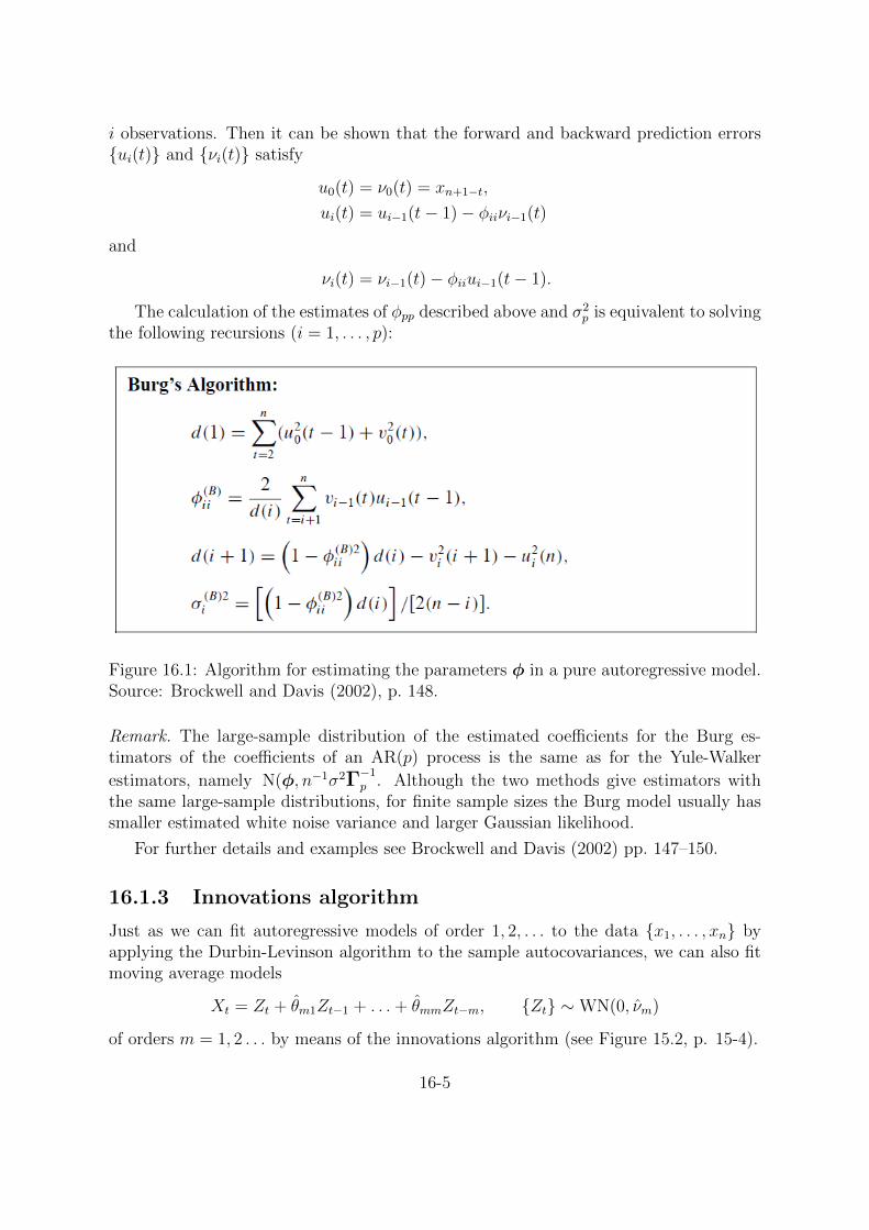
The calculation of the estimates of φpp described above and σ2p is equivalent to solving

the following recursions (i = 1, . . . , p):

Figure 16.1: Algorithm for estimating the parameters φ in a pure autoregressive model.Source: Brockwell and Davis (2002), p. 148.

Remark. The large-sample distribution of the estimated coefficients for the Burg es-timators of the coefficients of an AR(p) process is the same as for the Yule-Walker

estimators, namely N(φ, n−1σ2Γ−1p . Although the two methods give estimators withthe same large-sample distributions, for finite sample sizes the Burg model usually hassmaller estimated white noise variance and larger Gaussian likelihood.

For further details and examples see Brockwell and Davis (2002) pp. 147–150.

16.1.3 Innovations algorithm

Just as we can fit autoregressive models of order 1, 2, . . . to the data {x1, . . . , xn} byapplying the Durbin-Levinson algorithm to the sample autocovariances, we can also fitmoving average models

Xt = Zt + θm1Zt−1 + . . .+ θmmZt−m, {Zt} ∼WN(0, νm)

of orders m = 1, 2 . . . by means of the innovations algorithm (see Figure 15.2, p. 15-4).

16-5

Proposition 16.1.4. The fitted innovations MA(m) model is

Xt = Zt + θm1Zt−1 + . . .+ θmmZt−m, {Zt} ∼WN(0, νm),

where θm = (θm1, . . . , θmm) and νm are obtained from the innovations algorithm with theautocovariance function replaced by the sample autocovariance function.

Order selection Three useful techniques for selecting an appropriate MA model aregiven below. The third is more systematic and extends beyond the narrow class of puremoving-average models.

� We know that for an MA(q) process the autocorrelations ρ(m), m > q, are zero.Moreover, the sample autocorrelation ρm, m > q, is approximately normally dis-tributed with mean ρ(m) = 0 and variance

n−1[1 + 2ρ2(1) + . . . 2ρ2(q)

].

This result enables us to use the graph of ρ(m), m = 1, 2, . . . , both to decidewhether or not a given data set can be plausibly modeled by a moving-averageprocess and also to obtain a preliminary estimate of the order q as the smallestvalue of m such that ρ(k) is not significantly different from zero for all k > m. Forpractical purposes ρ(k) is compared to 1.96n−1/2 in absolute value.

� We examine the coefficient vectors θm, m = 1, 2, . . . to be able not only to assessthe appropriateness of a moving-average model and to estimate its order q, but alsoto obtain preliminary estimates θm1, . . . , θmq of the coefficients. By inspecting the

estimated coefficients θm1, . . . , θmm for m = 1, 2, . . . and the ratio of each coefficientestimate θmj to

1.96σj = 1.96n−1/2

(j−1∑

i=0

θ2mi

)1/2

,

we can see which of the coefficient estimates are most significantly different fromzero, estimate for order of the model to be fitted as the largest j for which theratio is larger than 1 in absolute value.

� As for autoregressive models, a more systematic approach to order selection formoving-average models is to find the values of q and θq = (θm1, . . . , θmq)

′ thatminimize the AICC statistic

AICC = −2 lnL

(θq,

S(θq)

n

)+

2(q + 1)n

n− q − 2,

where L is the Gaussian likelihood defined in (16.7) and S is defined in (16.8).

16-6

16.1.4 Hannan-Rissanen algorithm (1982)

The defining equations for a causal AR(p) model have the form of a linear regressionmodel with coefficient vector φ = (φ1, . . . , φp)

′. This suggests the use of simple leastsquares regression for obtaining preliminary parameter estimates when q = 0. Appli-cation of this technique when q > 0 is complicated by the fact that in the generalARMA(p, q) equations {Xt} is regressed not only on Xt−1, . . . , Xt−p, but also on theunobserved quantities Zt−1, . . . , Zt−q. Nevertheless, it is still possible to apply leastsquares regression to the estimation of φ and θ by first replacing the unobserved quanti-ties Zt−1, . . . , Zt−q by estimated values Zt−1, . . . , Zt−q. The parameters φ and θ are then

estimated by regressing Xt onto Xt−1, . . . , Xt−p, Zt−1, . . . , Zt−q. These are the main stepsin the Hannan-Rissanen estimation procedure, which we now describe in more detail.

Step 1: A high-order AR(m) model (with m > max(p, q)) is fitted to the data usingthe Yule-Walker estimates of Section 16.1.1. If (φm1, . . . , φmm)′ is the vector of estimatedcoefficients, then the estimated residuals are computed from the equations

Zt = Xt − φm1Xt−1 − . . .− φmmXt−m, t = m+ 1, . . . , n.

Step 2: Once the estimated residuals Zt, t = m + 1, . . . , n, have been computed asin Step 1, the vector of parameters β = (φ′,θ′) is estimated by least squares linearregression of Xt onto (Xt−1, . . . , Xt−p, Zt−1, . . . , Zt−q), t = m + 1 + q, . . . , n, i.e., byminimizing

S(β) =n∑

t=m+1+q

(Xt − φ1Xt−1 − . . .− φpXt−p − θ1Zt−1 − . . .− θqZt−q)2

with respect to β. This gives the Hannan-Rissanen estimator

β = (Z′Z)−1Z′Xn,

where Xn = (Xm+1+q, . . . , Xn)′ and Z is the (n−m− q)× (p+ q) matrix

Z =

Xm+q Xm+q−1 · · · Xm+q+1−p Zm+q · · · Zm+1

Xm+q+1 Xm+q · · · Xm+q+2−p Zm+q+1 · · · Zm+2

...... · · · ...

... · · · ...

Xn−1 Xn−2 · · · Xn−p Zn−1 · · · Zn−q

.

The Hannan-Rissanen estimate of the white noise variance is

σ2HR =

S(β)

n−m− q .

16-7

16.2 Maximum Likelihood Estimation

Suppose that {Xt} is a Gaussian time series with mean zero and autocovariance functionκ(i, j) = E(XiXj). Let Xn = (X1, . . . , Xn)′ and let Xn = (X1, . . . , Xn)′, where X1 = 0

and Xj = E(Xj|X1, . . . , Xj−1) = Pj−1Xj, j ≥ 2. Let Γn denote the covariance matrixΓn = E(XnX

′n), and assume that Γn is nonsingular.

The likelihood of Xn is

L(Γn) = (2π)−n/2(det Γn)−1/2 exp

(−1

2X ′nΓ

−1n Xn

). (16.5)

The direct calculation of det Γn and Γ−1n can be avoided by expressing this in termsof the one-step predictors Xj, and their mean squared errors νj−1, j = 1, . . . , n, both ofwhich are calculated recursively from the innovations algorithm.

It can be shown, that

X ′nΓ−1n Xn =

n∑

j=1

(Xj − Xj)2

νj−1,

and

det(Γn) = ν0 · . . . · νn−1.

The likelihood (16.5) of the vector Xn therefore reduces to

L(Γn) = (2π)−n/2(ν0 · . . . · νn−1)−1/2 exp

(−1

2

n∑

j=1

(Xj − Xj)2

νj−1

). (16.6)

Remark. Even if {Xt} is not Gaussian, it still makes sense to estimate the unknownparameters β = (φ1, . . . , φp, θ1, . . . θq)

′ in such a way as to maximize (16.6).A justification for using maximum Gaussian likelihood estimators of ARMA coef-

ficients is that the large-sample distribution of the estimators is the same for {Zt} ∼IID(0, σ2), regardless of whether or not {Zt} is Gaussian.

16.2.1 Estimation for ARMA processes

Suppose now that {Xt} is a causal ARMA(p, q) process. Applying the innovationsalgorithm ((15.8)) we find the one-step predictors Xi+1 and the mean squared errorsE(Xi+1 − Xi+1) = σ2ri. Substituting in the general expression (16.6), we find theGaussian likelihood of the vector of observations Xn = (X1, . . . , Xn)′.

Proposition 16.2.1. The Gaussian likelihood for an ARMA(p, q) process:

L(φ,θ, σ2) =1√

(2πσ2)n r0 · · · rn−1exp

(− 1

2σ2

n∑

j=1

(Xj − Xj)2

rj−1

)(16.7)

16-8

with rj = E(Xj+1 − Xj+1)2/σ2.

Differentiating lnL(φ,θ, σ2) partially with respect to σ2 and noting that Xj and rjare independent of σ2, we find that the maximum likelihood estimators φ, θ, and σ2

satisfy

σ2 = n−1S(φ, θ)

where

S(φ, θ) =n∑

j=1

(Xj − Xj)2

rj−1(16.8)

and φ, θ are the values of φ,θ that minimize

l(φ,θ) = ln(n−1S(φ,θ)) +1

n

n∑

j=1

ln rj−1. (16.9)

Remark. Minimization of l(φ,θ) must be done numerically. The search procedure maybe greatly accelerated if we begin with parameter values φ0,θ0 which are close to theminimum of l. It is for this reason that simple, reasonably good preliminary estimatesof φ,θ are important (see Section 16.1). It is essential to begin the search with a causalparameter vector φ0 since causality is assumed in the computation of l(φ,θ).

16.2.2 Order selection

Let {Xt} denote the mean-corrected transformed series. The problem now is to find themost satisfactory ARMA(p, q) model to represent {Xt}. If p and q were known in advancethis would be a straightforward application of the estimation techniques. However thisis usually not the case, so that it becomes necessary also to identify appropriate valuesfor p and q.

It might appear at first sight that the higher the values of p and q chosen, the betterthe fitted model will be. However we must beware of the danger of overfitting, i.e. oftailoring the fit too closely to the particular numbers observed.

Criteria have been developed, which attempt to prevent overfitting by effectivelyassigning a cost to the introduction of each additional parameter.

We choose a biased-corrected form of the Akaike’s AIC criterion, defined for anARMA(p, q) model with coefficients φp and θq, by

AICC = −2 lnL

(φp,θq,

S(φp,θq)

n

)+

2(p+ q + 1)n

n− p− q − 2,

where L(φ,θ, σ2) is the likelihood of the data under the Gaussian ARMA model (16.7)with parameters (φ,θ, σ2) and S(φ,θ) is the residual sum of squares (16.8). We selectthe model that minimizes the value of AICC. Intuitively one can think of 2(p + q +1)n/(n−p−q−2) as a penalty term to discourage over-parameterization. Once a modelhas been found which minimizes the AICC value, it must then be checked for goodnessof fit (essentially by checking that the residuals are like white noise) as discussed inSection 16.3.

16-9

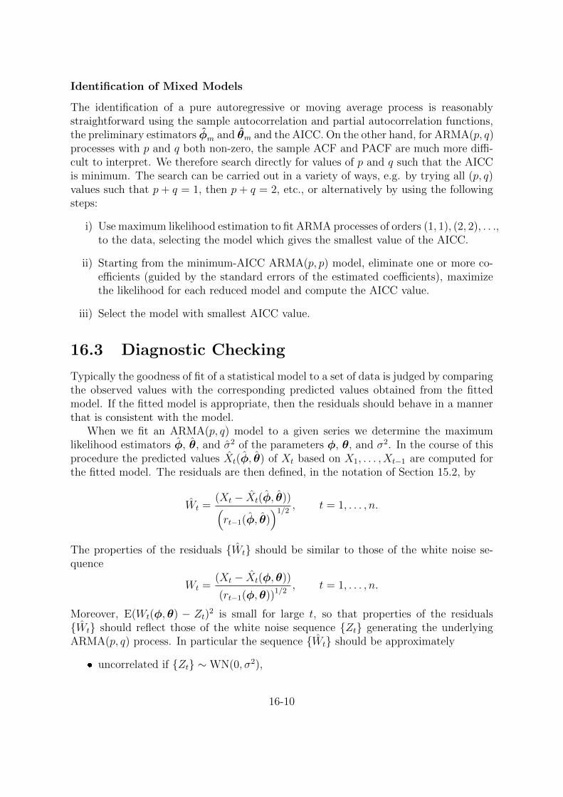
Identification of Mixed Models

The identification of a pure autoregressive or moving average process is reasonablystraightforward using the sample autocorrelation and partial autocorrelation functions,the preliminary estimators φm and θm and the AICC. On the other hand, for ARMA(p, q)processes with p and q both non-zero, the sample ACF and PACF are much more diffi-cult to interpret. We therefore search directly for values of p and q such that the AICCis minimum. The search can be carried out in a variety of ways, e.g. by trying all (p, q)values such that p + q = 1, then p + q = 2, etc., or alternatively by using the followingsteps:

i) Use maximum likelihood estimation to fit ARMA processes of orders (1, 1), (2, 2), . . .,to the data, selecting the model which gives the smallest value of the AICC.

ii) Starting from the minimum-AICC ARMA(p, p) model, eliminate one or more co-efficients (guided by the standard errors of the estimated coefficients), maximizethe likelihood for each reduced model and compute the AICC value.

iii) Select the model with smallest AICC value.

16.3 Diagnostic Checking

Typically the goodness of fit of a statistical model to a set of data is judged by comparingthe observed values with the corresponding predicted values obtained from the fittedmodel. If the fitted model is appropriate, then the residuals should behave in a mannerthat is consistent with the model.

When we fit an ARMA(p, q) model to a given series we determine the maximumlikelihood estimators φ, θ, and σ2 of the parameters φ, θ, and σ2. In the course of thisprocedure the predicted values Xt(φ, θ) of Xt based on X1, . . . , Xt−1 are computed forthe fitted model. The residuals are then defined, in the notation of Section 15.2, by

Wt =(Xt − Xt(φ, θ))(rt−1(φ, θ)

)1/2 , t = 1, . . . , n.

The properties of the residuals {Wt} should be similar to those of the white noise se-quence

Wt =(Xt − Xt(φ,θ))

(rt−1(φ,θ))1/2, t = 1, . . . , n.

Moreover, E(Wt(φ,θ) − Zt)2 is small for large t, so that properties of the residuals

{Wt} should reflect those of the white noise sequence {Zt} generating the underlyingARMA(p, q) process. In particular the sequence {Wt} should be approximately

� uncorrelated if {Zt} ∼WN(0, σ2),

16-10

� independent if {Zt} ∼ IID(0, σ2), and

� normally distributed if {Zt} ∼ N(0, σ2).

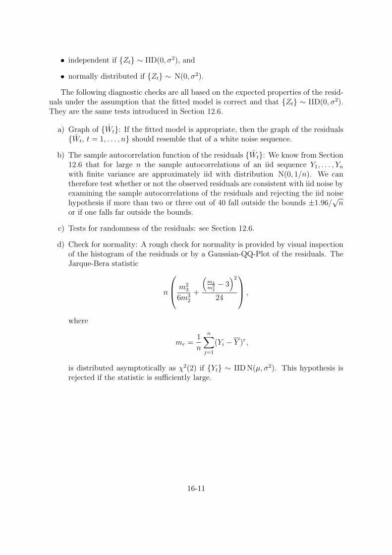
The following diagnostic checks are all based on the expected properties of the resid-uals under the assumption that the fitted model is correct and that {Zt} ∼ IID(0, σ2).They are the same tests introduced in Section 12.6.

a) Graph of {Wt}: If the fitted model is appropriate, then the graph of the residuals{Wt, t = 1, . . . , n} should resemble that of a white noise sequence.

b) The sample autocorrelation function of the residuals {Wt}: We know from Section12.6 that for large n the sample autocorrelations of an iid sequence Y1, . . . , Ynwith finite variance are approximately iid with distribution N(0, 1/n). We cantherefore test whether or not the observed residuals are consistent with iid noise byexamining the sample autocorrelations of the residuals and rejecting the iid noisehypothesis if more than two or three out of 40 fall outside the bounds ±1.96/

√n

or if one falls far outside the bounds.

c) Tests for randomness of the residuals: see Section 12.6.

d) Check for normality: A rough check for normality is provided by visual inspectionof the histogram of the residuals or by a Gaussian-QQ-Plot of the residuals. TheJarque-Bera statistic

n

m2

3

6m32

+

(m4

m32− 3)2

24

,

where

mr =1

n

n∑

j=1

(Yi − Y )r,

is distributed asymptotically as χ2(2) if {Yt} ∼ IID N(µ, σ2). This hypothesis isrejected if the statistic is sufficiently large.

16-11

Defi

nit

ion

:{X

t}is

anA

RM

A(p,q

)pr

oces

sif{X

t}is

stat

iona

ryan

dif

for

ever

yt,

Xt−φ1Xt−

1−...−

φpXt−p

=Zt

+θ 1Zt−

1+...+

θ qZt−q,

whe

re{Z

t}∼

WN

(0,σ

2)

and

the

pol

ynom

ialsφ

(z)

andθ(z)

have

noco

mm

onfa

ctor

s.

Ifφ

(z)≡

1,th

enth

epr

oces

sis

said

tob

ea

mov

ing-

aver

age

proc

ess

ofor

derq

orM

A(q

).

Ifθ(z)≡

1th

enth

epr

oces

sis

said

tob

ean

auto

regr

essi

vepr

oces

sof

orde

rp

orA

R(p

).

AR

(p)

MA

(q)

AR

MA

(p,q

)M

od

elXt

=φ1Xt−

1+...+

φpXt−p

+Zt

Xt

=Zt

+θ 1Zt−

1+...+

θ qZt−q

Xt−φ1Xt−

1−...−

φpXt−p

=Zt

+θ 1Zt−

1+...+

θ qZt−q

φ(B

)Xt

=Zt

Xt

=θ(B

)Zt

φ(B

)Xt

=θ(B

)Zt

Sta

tion

arit

yA

R(1

):|φ|

<1

per

defin

itio

nif

and

only

ifφ

(z)

=1−φ1z−...−

φpzp6=

0fo

ral

l|z|

=1

Cau

sality

Defi

niti

onth

ere

exis

tco

nsta

nts{ψ

j}s

uch

that∑∞ j=

0|ψj|<∞

and

Xt

=∑∞ j=

0ψjZt−j

for

allt

Pro

pos

itio

np

erde

finit

ion

ifan

don

lyifφ

(z)

=1−φ1z−...−

φpzp6=

0fo

ral

l|z|≤

1C

oeffi

cien

tsT

heco

effici

ents{ψ

j}a

rede

term

ined

byth

ere

lati

onψ

(z)

=∑∞ j=

0ψjzj

=θ(z)/φ

(z),

|z|≤

1

Inve

rtib

ilit

yD

efini

tion

ther

eex

ist

cons

tant

s{π

j}s

uch

that∑∞ j=

0|π j|<∞

and

Zt

=∑∞ j=

0π jXt−j

for

allt

Pro

pos

itio

np

erde

finit

ion

ifan

don

lyifθ(z)

=1

+θ 1z

+...+

θ qzq6=

0fo

ral

l|z|≤

1C

oeffi

cien

tsT

heco

effici

ents{π

j}a

rede

term

ined

byth

ere

lati

onπ

(z)

=∑∞ j=

0π jzj

=φ

(z)/θ(z),

|z|≤

1

AC

FA

R(1

):ρ(h)

=φ|h|

AR

(p):

deca

ysρ(h)

=

∑q−|h|

j=

0θ jθ j

+|h|

∑q j=

0θ2 j

if|h|≤q

0if|h|

>q

infin

ite

finit

ein

finit

e(d

amp

edex

pon

enti

als

and/

orsi

new

aves

afte

rfir

stq−p

lags

)

PA

CF

MA

(1)

:α(h

)=−(−θ

)h(1−θ

2)

1−θ2

(h+

1)

α(h

)=

{ φp

ifh

=p

0ifh>p

MA

(q):

deca

ys

finit

ein

finit

ein

finit

e(d

amp

edex

pon

enti

als

and/

orsi

new

aves

afte

rfir

stp−q

lage

s)

Figure 16.2: Summary of the ARMA time series models

16-12

17 Nonstationary and SeasonalTime Series Models

If the data (a) exhibit no apparent deviations from stationarity and (b) have a rapidlydecreasing autocovariance function, we attempt to fit an ARMA model to the mean-corrected data using the techniques developed in Chapter 16. Otherwise, we look firstfor a transformation of the data that generates a new series with the properties (a) and(b). This can frequently be achieved by differencing, leading us to consider the class ofARIMA (autoregressive integrated moving-average) models.

17.1 ARIMA Models

Definition 17.1.1. If d is a non-negative integer, then {Xt} is an ARIMA(p, d, q) processif

Yt := (1−B)dXt

is a causal ARMA(p, q) process.

Remark. This definition means that {Xt} satisfies a difference equation of the form

φ?(B)Xt ≡ φ(B)(1−B)dXt = θ(B)Zt, {Zt} ∼WN(0, σ2), (17.1)

where φ(z) and θ(z) are polynomials of degrees p and q, respectively, and φ(z) 6= 0 for|z| ≤ 1. The polynomial φ?(z) has a zero of order d at z = 1. The process {Xt} isstationary if and only if d = 0, in which case it reduces to an ARMA(p, q) process.

Remark. Notice that if d ≥ 1, we can add an arbitrary polynomial trend of degree (d−1)to {Xt} without violating the difference equation (17.1). ARIMA models are thereforeuseful for representing data with trend.

17.2 SARIMA Models

We have already seen how differencing the series {Xt} at lag s is a convenient way ofeliminating a seasonal component of period s. If we fit an ARMA(p, q) model φ(B)Yt =θ(B)Zt to the differenced series Yt = (1− Bs)Xt, then the model for the original seriesis φ(B)(1 − Bs)Xt = θ(B)Zt. This is a special case of the general seasonal ARIMA(SARIMA) model defined as follows.

The background idea of the application of SARIMA models can be described in threesteps (see Schlittgen and Streitberg (2001)).

1. The existence of seasonal effects means, that an observation of a specific monthdepends on the observations of the same month for past years (e.g. January 2010depends on January 2009, January 2008 etc.). Considering the observations of the

17-1

same month (data with lag s = 12), these dependency can be modeled with anARIMA process: Φ(Bs)(1 − Bs)DXt = Θ(Bs)Ut, where {Xt} is the original timeseries, e.g. the Basel monthly mean temperature time series from 1900 to 2010.

2. Ut is not a White-noise process since there is also a dependency of the tempera-tures between successive months (e.g. January 2010 depends on December 2009,November 2009 etc.). Therefore these non-seasonal patterns are also modeled withan ARIMA process: φ(B)(1−B)dUt = θ(B)Zt, where Zt is a white-noise process.

3. Multiplying the first equation with φ(B)(1−B)d and applying the second equationwe get

φ(B)(1−B)dΦ(Bs)(1−Bs)DXt = φ(B)(1−B)dΘ(Bs)Ut = θ(B)Θ(Bs)Zt.

Definition 17.2.1. If d and D are non-negative integers then {Xt} is a

seasonal ARIMA(p, d, q)× (P,D,Q)s process

with period s if the differenced series

Yt := (1−B)d(1−Bs)DXt

is a causal ARMA(p, q) process defined by

φ(B)Φ(Bs)Yt = θ(B)Θ(Bs)Zt, {Zt} ∼WN(0, σ2), (17.2)

where

φ(z) = 1− φ1z − . . .− φpzp,Φ(z) = 1− Φ1z − . . .− ΦP z

P ,

θ(z) = 1 + θ1z + . . .+ θqzq,

Θ(z) = 1 + Θ1z + . . .+ ΘQzQ.

Example (Basel, p. 1-6). Since the autocorrelation function of Figure 12.10, p. 12-19,showed among other things a negative correlation at lag 12 after differencing the Baselmonthly mean temperature time series with (1−B)(1−B12), we will now use a SARIMAprocess to find an adequate model. Applying an ARIMA(1, 1, 1) × (1, 1, 1)12 processresults in Figure 17.1 which shows that the residuals are white noise and therefore themodel is appropriate. Finally Table 17.1 shows the results of the parameter estimation.

Remark. Note that the process {Yt} is causal if and only if φ(z) 6= 0 and Θ(z) 6= 0 for|z| ≤ 1. In applications D is rarely more than one, and P and Q are typically less thanthree.

17-2

Plot of Residuals

-10

-50

5

Jan 1750 Jan 1800 Jan 1850 Jan 1900 Jan 1950 Jan 2000ACF Plot of Residuals

AC

F

0.0 0.5 1.0 1.5 2.0 2.5 3.0-1.0

0.0

1.0

PACF Plot of Residuals

PA

CF

0.0 0.5 1.0 1.5 2.0 2.5 3.0-0.0

40.

00.

04

P-values of Ljung-Box Chi-Squared Statistics

Lag

p-va

lue

0.4 0.6 0.8 1.0 1.2

0.0

0.4

0.8

ARIMA Model Diagnostics: bmII.om

ARIMA() Model with Mean 0Figure 17.1: Residuals of the Basel monthly mean temperature time series from 1900 to2010 after applying a seasonal ARIMA(1, 1, 1)× (1, 1, 1)12 process.

Remark. The equation (17.2) can be rewritten in the equivalent form

φ?(B)Yt = θ?(B)Zt,

where φ?(·) and θ?(·) are polynomials of degree p+sP and q+sQ, respectively, whose co-efficients can all be expressed in terms of φ1, . . . , φp,Φ1, . . . ,ΦP , θ1, . . . , θq, and Θ1, . . . ,ΘQ.

Remark. In Section 12.5 we discussed the classical decomposition model incorporatingtrend, seasonality, and random noise. In modeling real data it might not be reasonable toassume, as in the classical decomposition model, that the seasonal component st repeatsitself precisely in the same way cycle after cycle. SARIMA models allow for randomnessin the seasonal pattern from one cycle to the next.

17-3

Table 17.1: Parameter estimation of the seasonal ARIMA(1, 1, 1)× (1, 1, 1)12 process.

17-4