15-853:Algorithms in the Real World

Satisfiability Solvers (Lectures 1 & 2)

1

Satisfiability (SAT)

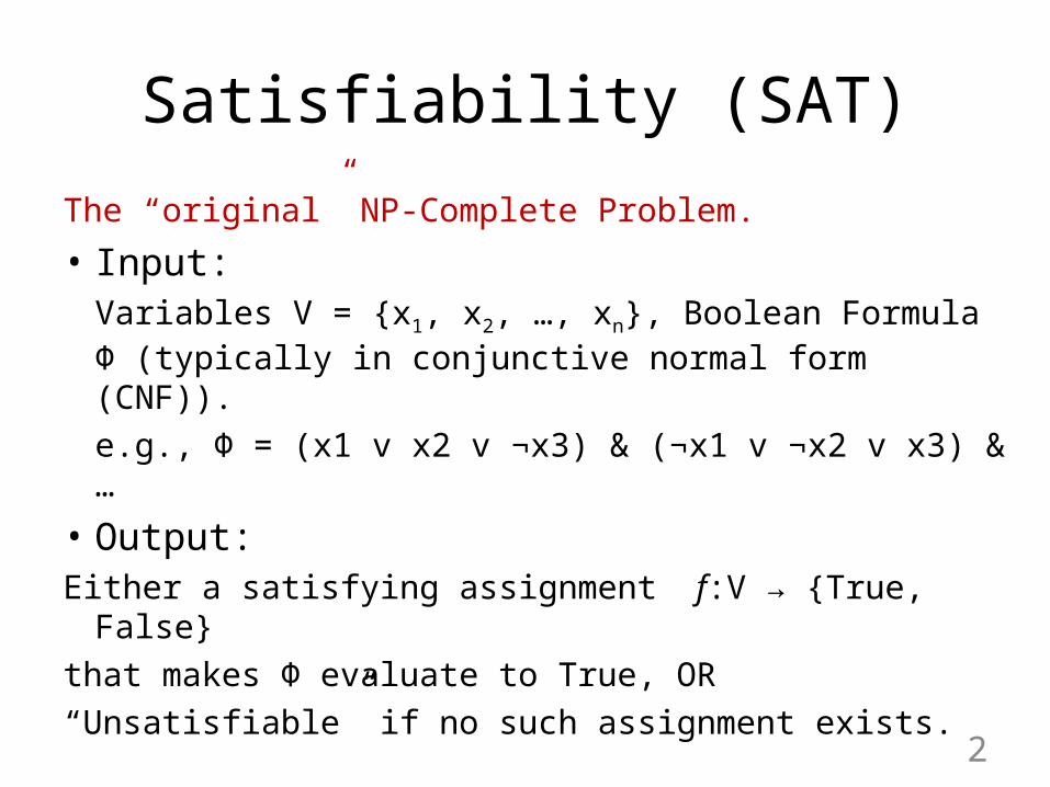
The “original” NP-Complete Problem.

• Input: Variables V = {x1, x2, …, xn}, Boolean Formula Φ (typically in conjunctive normal form (CNF)).e.g., Φ = (x1 v x2 v ¬x3) & (¬x1 v ¬x2 v x3) & …

• Output: Either a satisfying assignment f:V → {True, False} that makes Φ evaluate to True, OR“Unsatisfiable” if no such assignment exists.

2

Extensions/Related Problems

• Satisfiability Modulo TheoriesInput: a formula Φ in quantifier-free first-order logic.Output: is Φ satisfiable?

• Theorem Provers• Pseudo-boolean optimization• Planners (Quantified SAT Solvers)

3

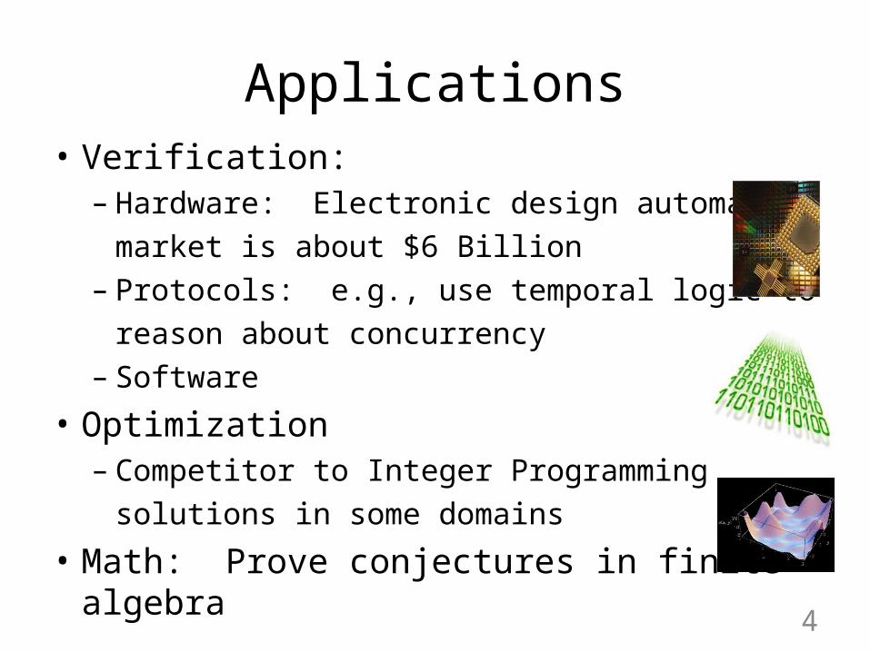
Applications• Verification:

– Hardware: Electronic design automation market is about $6 Billion

– Protocols: e.g., use temporal logic to reason about concurrency

– Software

• Optimization– Competitor to Integer Programming

solutions in some domains

• Math: Prove conjectures in finite algebra 4

An Aside: Example Proof by Machine

• Thm: Robbins Algebra = Boolean Algebra• Robbins Algebra: values {0,1} and 3 axioms:

x v (y v z) = (x v y) v zx v y = y v z¬ (¬(x v y) v ¬(x v ¬y)) = x

• Conjectured in 1933• Proved in 1996 by prover EQP running for 8 days

(RS/6000 with ~30 MB RAM)• Limited success since 1990s.

5

Annual Competitions• SAT Competition • CADE ATP System Competition• ASP Solver Competition • SMT-COMP • Constraint Satisfaction Solver Competition • Competitition/Exhibition of Termination Tools • TANCS • QBF Solvers Evaluation • Open Source Solvers: SATLIB, SATLive

6

Algorithms for SAT

• Complete (satisfying assignment or UNSAT)– Davis-Putnam-Logemann-Loveland algorithm (DPLL)

• Incomplete (satisfying assignment or FAILURE)– GSAT– WalkSAT

7

Prerequisite: Proof Systems• What constitutes a proof of unsatisfiability?• For a language L in {0,1}*, a proof system for

membership in L is a poly-time computable function P such that – For all x in L, there is a witness y with P(x,y) = 1– For all x not in L, for all y, P(x,y) = 0

• Complexity: worst case length of shortest witness for an x in L.

8

Proof System Examples

• L = satisfiable boolean formulae• What’s the lowest complexity proof system for

this you can come up with?• What about for L = unsatisfiable boolean

formulae?

9

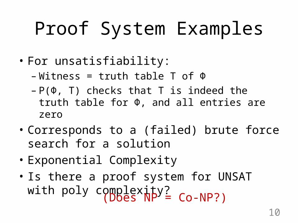
Proof System Examples

• For unsatisfiability:– Witness = truth table T of Φ– P(Φ, T) checks that T is indeed the truth table for Φ,

and all entries are zero

• Corresponds to a (failed) brute force search for a solution

• Exponential Complexity• Is there a proof system for UNSAT with poly

complexity?10

(Does NP = Co-NP?)

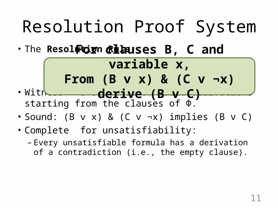
• The Resolution Rule:

• Witness = a sequence of valid derivations starting from the clauses of Φ.

• Sound: (B v x) & (C v ¬x) implies (B v C)• Complete for unsatisfiability:

– Every unsatisfiable formula has a derivation of a contradiction (i.e., the empty clause).

For clauses B, C and variable x,From (B v x) & (C v ¬x) derive (B v C)

Resolution Proof System

11

Duality

• Truth table proof system gives proofs by failed search for a satisfying assignment.

• Resolution proof system gives proofs by showing the initial clauses (constraints) yield a contradiction. This is a systematic search for additional constraints the solution must satisfy.

12

High level idea for many solvers

• Alternate search for solution with search for properties of any solution:– Search for solution in some small part S of the space– If search in S fails, search for a reason for this failure,

in the form of a new constraint C the solution must satisfy.

– Search for a solution in a new part of the space, using new constraint to help guide the search

– Repeat

13

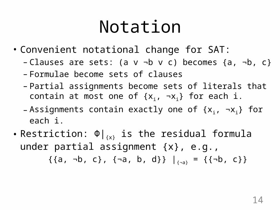
Notation• Convenient notational change for SAT:

– Clauses are sets: (a v ¬b v c) becomes {a, ¬b, c}– Formulae become sets of clauses– Partial assignments become sets of literals that contain

at most one of {xi, ¬xi} for each i.

– Assignments contain exactly one of {xi, ¬xi} for each i.

• Restriction: Φ|{x} is the residual formula under partial assignment {x}, e.g.,

{{a, ¬b, c}, {¬a, b, d}} |{¬a} = {{¬b, c}}

14

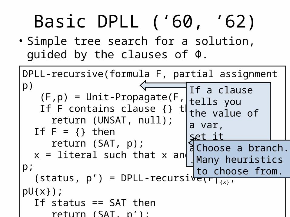
Basic DPLL (‘60, ‘62)• Simple tree search for a solution, guided by

the clauses of Φ.

15

DPLL-recursive(formula F, partial assignment p) (F,p) = Unit-Propagate(F, p); If F contains clause {} then

return (UNSAT, null); If F = {} then

return (SAT, p); x = literal such that x and ¬x are not in p; (status, p’) = DPLL-recursive(F|{x}, pU{x}); If status == SAT then

return (SAT, p’); Else return

DPLL-recursive(F|{¬x}, pU{¬x});

If a clause tells you the value of a var, set it appropriately.

Choose a branch.Many heuristicsto choose from.

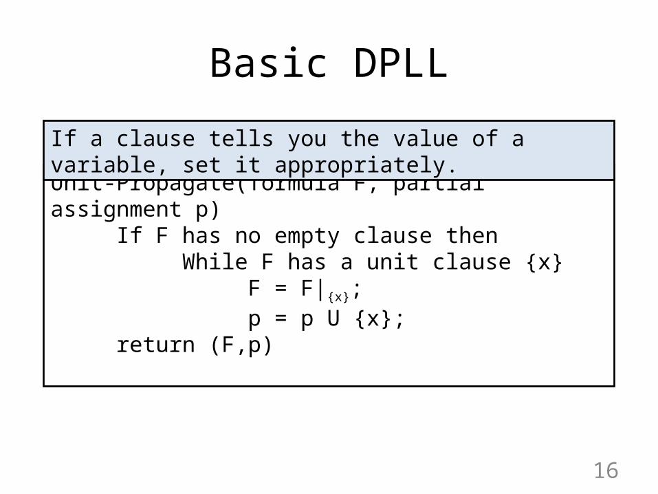
Basic DPLL

16

Unit-Propagate(formula F, partial assignment p)If F has no empty clause then

While F has a unit clause {x}F = F|{x};p = p U {x};

return (F,p)

If a clause tells you the value of a variable, set it appropriately.

Embellishing DPLL

• Branch Selection Heuristics• Clause Learning• Backjumping heuristics• Watched literals• Randomized Restarts• Symmetry breaking• More powerful proof systems• …

17

Branch Selection Heuristics

• Random• Max occurrence in clauses of min size• Max occurrence in as yet unsatisfied clauses• With probability proportional to some

function of how often the literal appears in partial assignments that lead to unsatisfiable restricted formulae.

• …

18

Clause Learning

• When DPLL discovers F|p is unsatisfiable, it derives (learns) a reason for this in the form of new clauses to add to F.

• What clauses are learned, and how, make huge differences in performance.

• Trivially learned clause: if F|p is unsatisfiable for

p = {x1, x2, …, xk}, derive clause {¬x1, ¬x2, …, ¬xk}

But we want short clauses that constrain the solution space as much as possible…

19

Clause Learning

• Use the clauses to guide the search:– So far we’ve seen unit-propagation, and search with

restriction.– We want to learn clauses that let us prune

effectively – this requires us to deduce “higher level” reasons why some partial assignment is no good.

– Use resolution (or some technique) to try to prove that F|p is unsatisfiable for nodes p high up the tree.

20

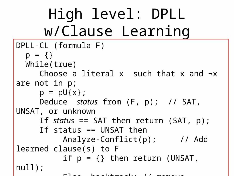
High level: DPLL w/Clause Learning

21

DPLL-CL (formula F) p = {} While(true)

Choose a literal x such that x and ¬x are not in p; p = pU{x};Deduce status from (F, p); // SAT, UNSAT, or unknown

If status == SAT then return (SAT, p); If status == UNSAT then

Analyze-Conflict(p); // Add learned clause(s) to Fif p = {} then return (UNSAT, null);

Else backtrack; // remove literals from p // based on learned clause(s)

If status == unknown then continue; // branch again

Deduce

• Tradeoff between searching more partial assignments (going deeper in the tree), and searching for proofs of unsatisfiability higher up in the tree.

• Currently, deduction is typically just iterated unit-propagation. (Other embellishments to DPLL seem to render more complex deduction unhelpful in practice.)

22

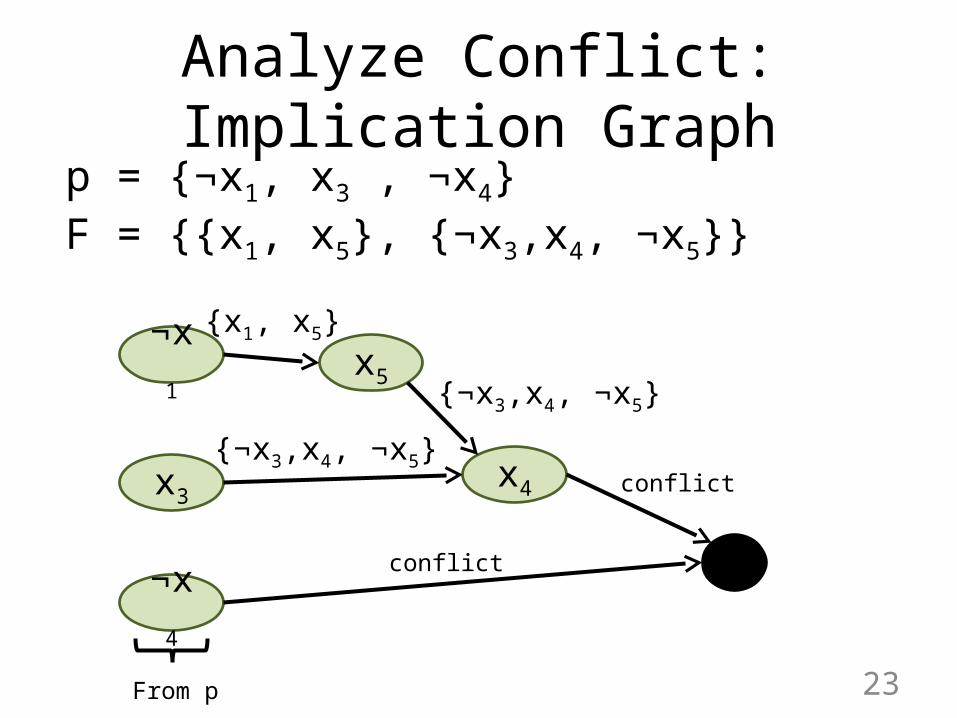
Analyze Conflict: Implication Graph

23

¬x1

x3

¬x4

p = {¬x1, x3 , ¬x4}F = {{x1, x5}, {¬x3,x4, ¬x5}}

x5

{x1, x5}

x4

{¬x3,x4, ¬x5}

{¬x3,x4, ¬x5}

From p

conflict

conflict

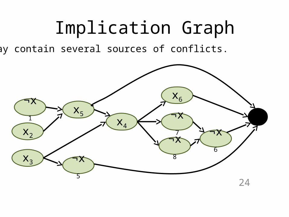
Implication Graph

24

¬x1

x2

¬x5

x5x4

May contain several sources of conflicts.

x6

¬x7

x3

¬x8

¬x6

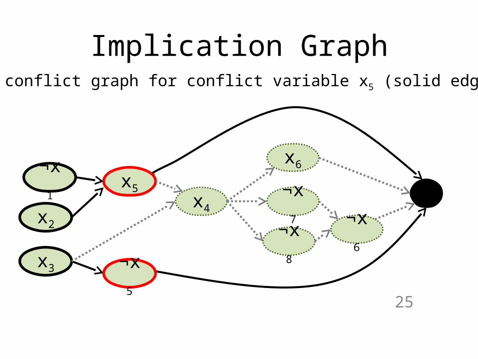
Implication Graph

25

¬x1

x2

¬x5

x5x4

x6

¬x7

x3

¬x8

¬x6

The conflict graph for conflict variable x5 (solid edges).

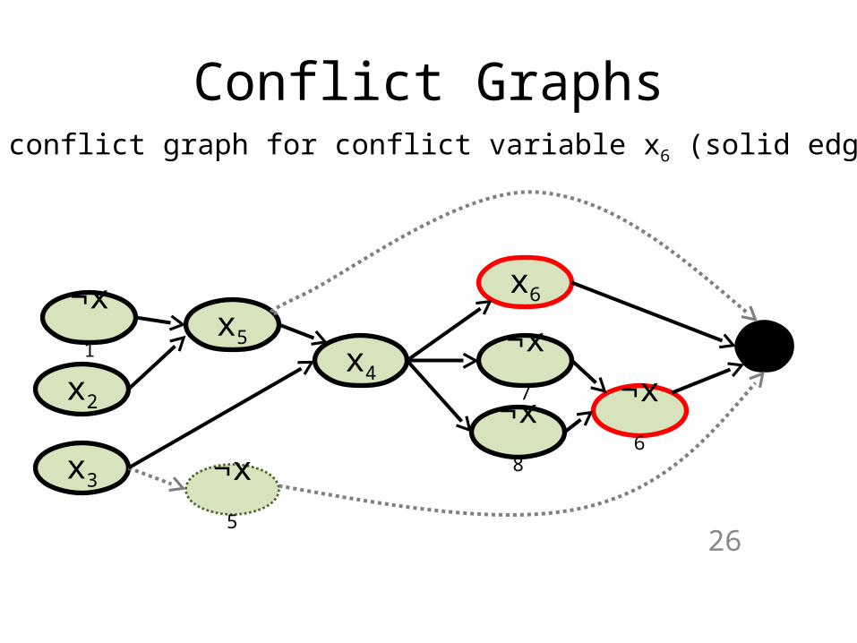
Conflict Graphs

26

¬x1

x2

¬x5

x5x4

The conflict graph for conflict variable x6 (solid edges).

x6

¬x7

x3

¬x8

¬x6

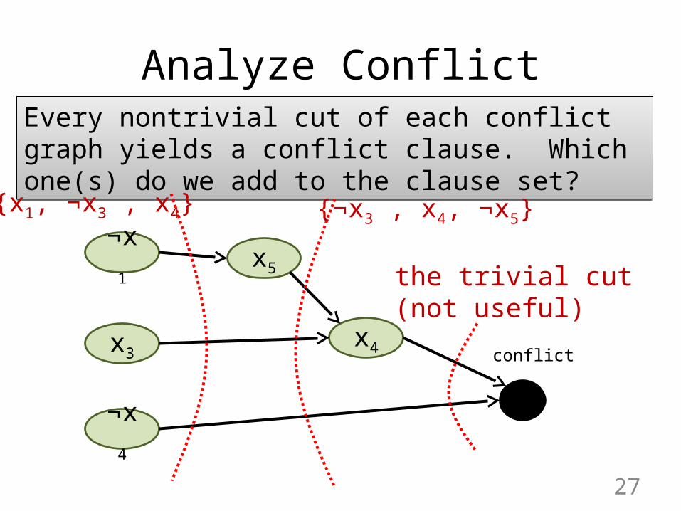
Analyze Conflict

27

¬x1

x3

¬x4

x5

x4 conflict

Every nontrivial cut of each conflict graph yields a conflict clause. Which one(s) do we add to the clause set?Every nontrivial cut of each conflict graph yields a conflict clause. Which one(s) do we add to the clause set?

{x1, ¬x3 , x4} {¬x3 , x4, ¬x5}

the trivial cut(not useful)

What Clauses to Learn?

• Can’t keep everything -- space is a major bottleneck in practice.

• Various heuristics:– First unique implication point– First new cut– Decision cut– …

28

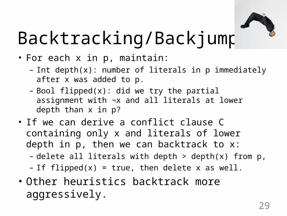
Backtracking/Backjumping

• For each x in p, maintain:– Int depth(x): number of literals in p immediately after x

was added to p.– Bool flipped(x): did we try the partial assignment with ¬x

and all literals at lower depth than x in p?

• If we can derive a conflict clause C containing only x and literals of lower depth in p, then we can backtrack to x:– delete all literals with depth > depth(x) from p,– If flipped(x) = true, then delete x as well.

• Other heuristics backtrack more aggressively.29

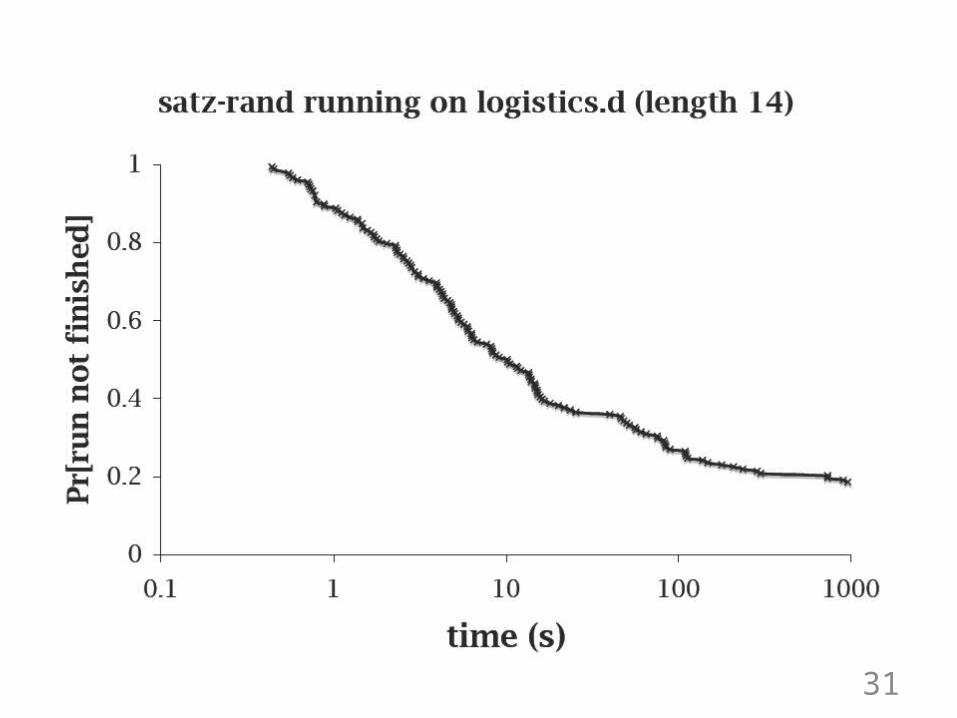
Random Restarts

• Restart: keep learned clauses, but throw away p, resample random bits, and start again.

• Essentially a very aggressive backjump.• Can help performance a lot.

– Run time distributions appear to be heavy-tailed.

30

31

Random Restarts: Heuristics• Fixed cutoff (always restart after T seconds)• Cutoff after k restarts is some function f(k)• Luby et. al. universal restart strategy for f(k)• f(k) = c*k, c^k, …• Restart policies based on predictive models of

solver behavior:– Bayesian approaches, Dynamic Programming, – Online submodular function maximization*

32

Embellishing DPLL

• Branch Selection Heuristics• Clause Learning• Backjumping heuristics• Watched literals• Randomized Restarts• Symmetry breaking• More powerful proof systems• …

33

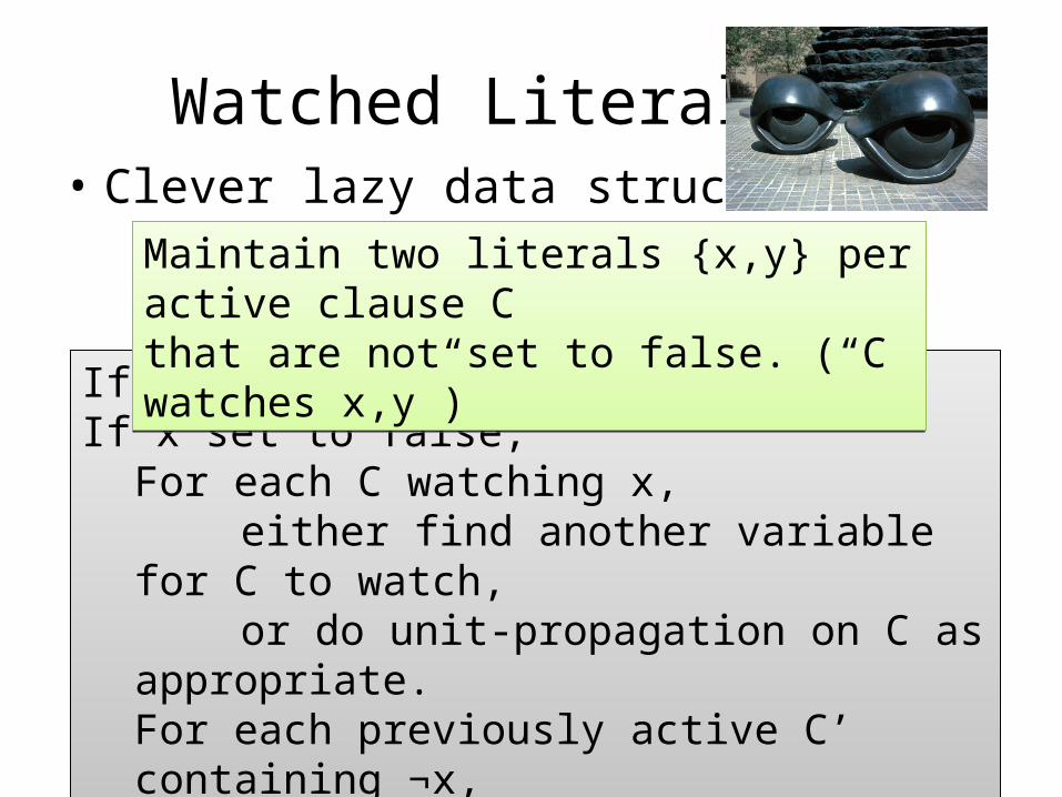
Watched Literals• Clever lazy data structure

34

If x set to true, do nothingIf x set to false,

For each C watching x, either find another variable for C to watch, or do unit-propagation on C as appropriate.

For each previously active C’ containing ¬x, set C’ to watch ¬x

If x is unset, do nothing (!)

If x set to true, do nothingIf x set to false,

For each C watching x, either find another variable for C to watch, or do unit-propagation on C as appropriate.

For each previously active C’ containing ¬x, set C’ to watch ¬x

If x is unset, do nothing (!)

Maintain two literals {x,y} per active clause C that are not set to false. (“C watches x,y”)Maintain two literals {x,y} per active clause C that are not set to false. (“C watches x,y”)

Watched Literals

• Helps quickly find if a clause is satisfied (just look at its watched literals)

• Helps quickly identify clauses ripe for unit-propagation.

• “now a standard method used by most SAT solvers for efficient constraint propagation” – Gomes et. al. “Satisfiability Solvers”

• Partially explains why deduce step is typically just iterated unit-propagation

35

Symmetry Breaking

• Symmetry is common in practice (e.g., identical trucks in vehicle routing)

• SAT encoding throws away this info.• Symmetry is useful for some proofs:

– e.g., Pigeon-hole principle: Impossible to place (n+1) birds into n bins, such that each bin gets at most one bird.

36

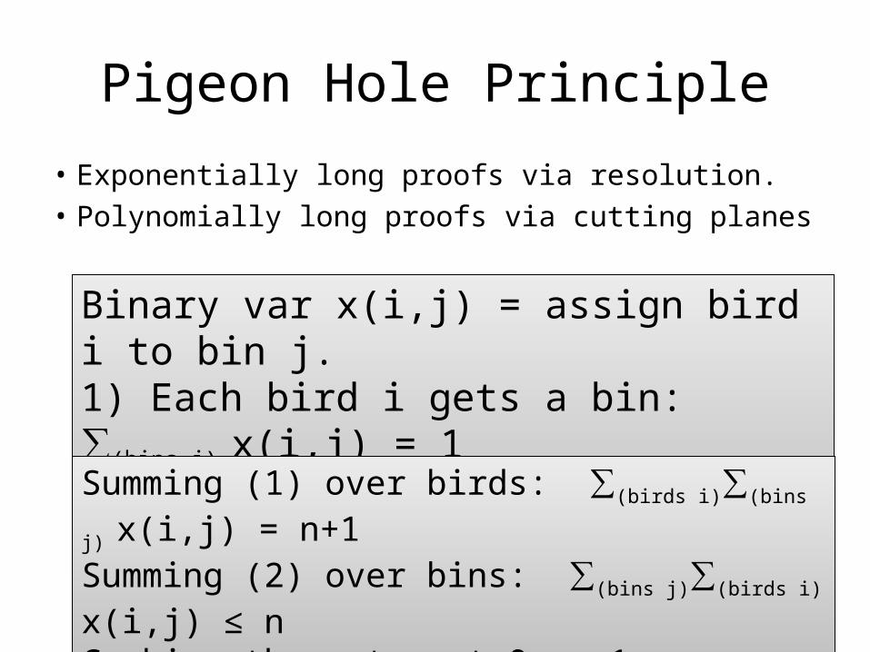
Pigeon Hole Principle

• Exponentially long proofs via resolution.• Polynomially long proofs via cutting planes

37

Binary var x(i,j) = assign bird i to bin j.1) Each bird i gets a bin: ∑(bins j) x(i,j) = 12) Each bin j has capacity one: ∑(birds i) x(i,j) ≤ 1

Binary var x(i,j) = assign bird i to bin j.1) Each bird i gets a bin: ∑(bins j) x(i,j) = 12) Each bin j has capacity one: ∑(birds i) x(i,j) ≤ 1

Summing (1) over birds: ∑(birds i)∑(bins j) x(i,j) = n+1Summing (2) over bins: ∑(bins j)∑(birds i) x(i,j) ≤ nCombine these to get 0 ≤ -1.

Summing (1) over birds: ∑(birds i)∑(bins j) x(i,j) = n+1Summing (2) over bins: ∑(bins j)∑(birds i) x(i,j) ≤ nCombine these to get 0 ≤ -1.

Symmetry Breaking

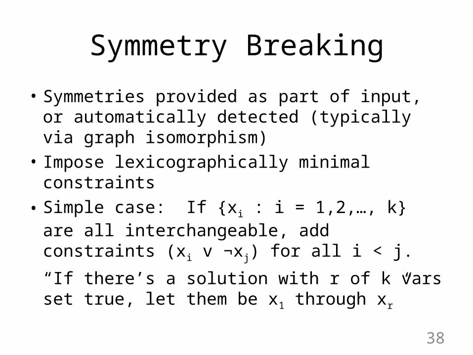
• Symmetries provided as part of input, or automatically detected (typically via graph isomorphism)

• Impose lexicographically minimal constraints• Simple case: If {xi : i = 1,2,…, k} are all

interchangeable, add constraints (xi v ¬xj) for all i < j.“If there’s a solution with r of k vars set true, let them be x1 through xr”

38

Symmetry Breaking

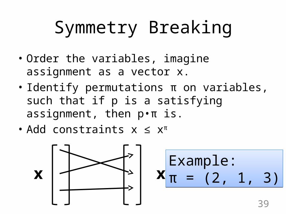
• Order the variables, imagine assignment as a vector x.

• Identify permutations π on variables, such that if p is a satisfying assignment, then p•π is.

• Add constraints x ≤ xπ

39

x xπExample:π = (2, 1, 3)Example:π = (2, 1, 3)

Other Proof Systems

• Truth Tables• Frege Systems (includes resolution as a special case)

• Extended Resolution: Add new vars• Resolution w/symmetry detection• Geometric systems (infer cutting planes)• …

40

Incomplete Algorithms

• Returns satisfying assignment or FAILURE• Based on heuristic search for a solution• Faster than complete algorithms for many

classes of satisfiable instances.• Examples:

– GSAT, WalkSAT, – Survey Propagation/Belief Propagation– Local search algs, Simulated Annealing, ILP, …

41

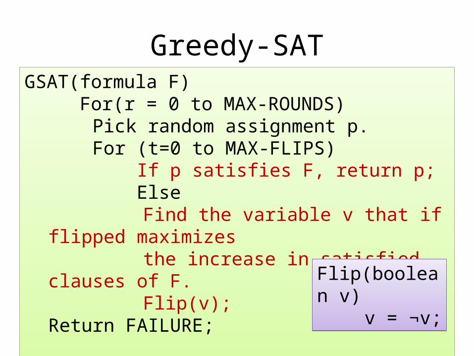
Greedy-SAT

42

GSAT(formula F) For(r = 0 to MAX-ROUNDS)

Pick random assignment p. For (t=0 to MAX-FLIPS) If p satisfies F, return p; Else

Find the variable v that if flipped maximizes

the increase in satisfied clauses of F.Flip(v);

Return FAILURE;

GSAT(formula F) For(r = 0 to MAX-ROUNDS)

Pick random assignment p. For (t=0 to MAX-FLIPS) If p satisfies F, return p; Else

Find the variable v that if flipped maximizes

the increase in satisfied clauses of F.Flip(v);

Return FAILURE;

Flip(boolean v)v = ¬v;

Flip(boolean v)v = ¬v;

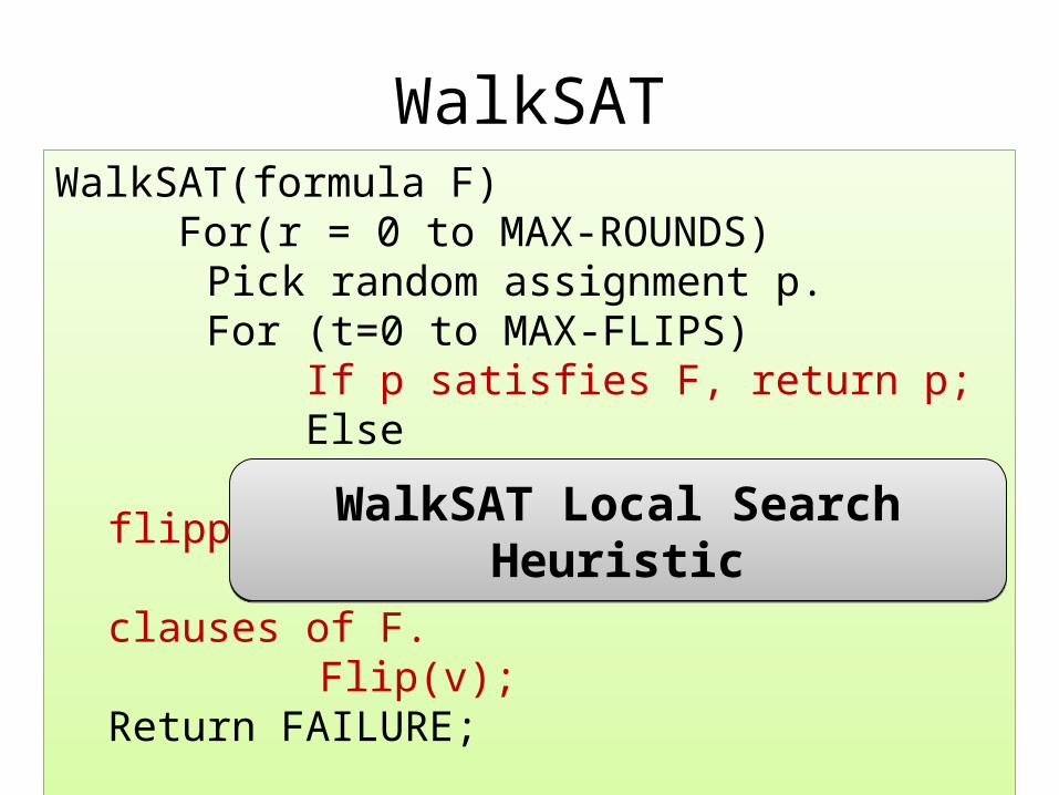
WalkSAT

43

WalkSAT(formula F) For(r = 0 to MAX-ROUNDS)

Pick random assignment p. For (t=0 to MAX-FLIPS) If p satisfies F, return p; Else

Find the variable v that if flipped maximizes

the increase in satisfied clauses of F.Flip(v);

Return FAILURE;

WalkSAT(formula F) For(r = 0 to MAX-ROUNDS)

Pick random assignment p. For (t=0 to MAX-FLIPS) If p satisfies F, return p; Else

Find the variable v that if flipped maximizes

the increase in satisfied clauses of F.Flip(v);

Return FAILURE;

WalkSAT Local Search HeuristicWalkSAT Local Search Heuristic

WalkSAT Local Search Heuristic

44

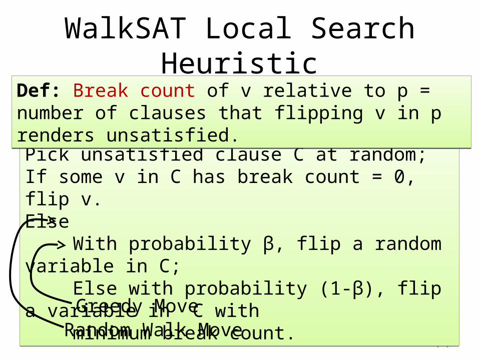
Pick unsatisfied clause C at random;If some v in C has break count = 0, flip v.Else

With probability β, flip a random variable in C;Else with probability (1-β), flip a variable in C with minimum break count.

Pick unsatisfied clause C at random;If some v in C has break count = 0, flip v.Else

With probability β, flip a random variable in C;Else with probability (1-β), flip a variable in C with minimum break count.

Def: Break count of v relative to p = number of clauses that flipping v in p renders unsatisfied. Def: Break count of v relative to p = number of clauses that flipping v in p renders unsatisfied.

Greedy MoveRandom Walk Move

Survey Propagation

• Derived from the cavity method in statistical physics.

• Like DPLL with a special branching heuristic: belief-propagation on objects related to SAT solutions (“covers”)

• Works really well in practice on some random instances – unclear why.

45

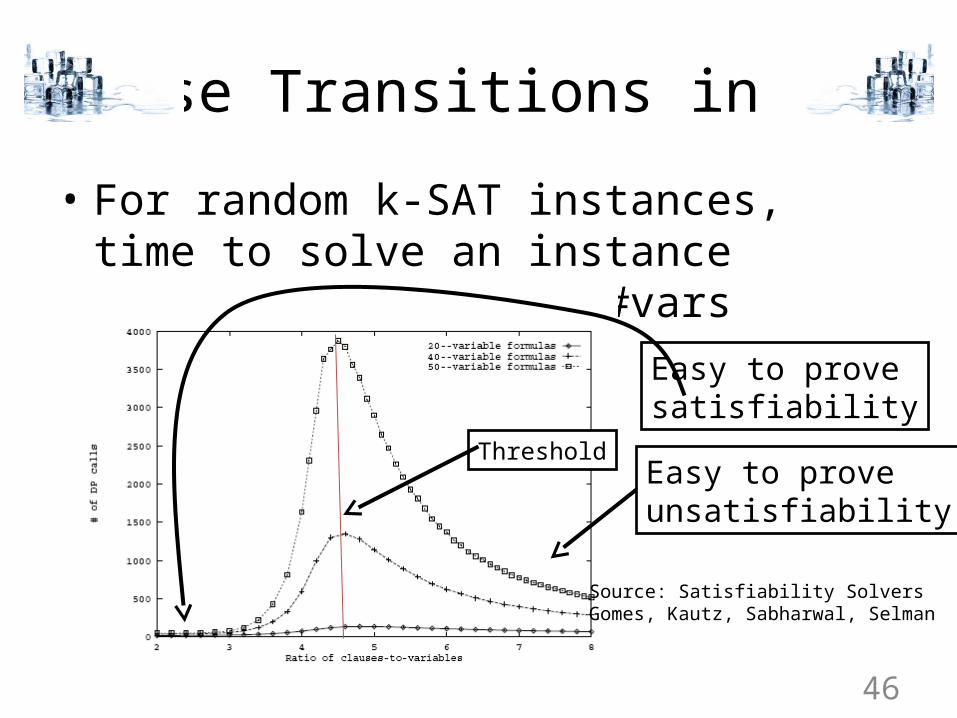
Phase Transitions in SAT

• For random k-SAT instances, time to solve an instance depends on #clauses/#vars

46

Source: Satisfiability SolversGomes, Kautz, Sabharwal, Selman

Easy to prove unsatisfiability

Easy to prove satisfiability

Threshold

Backdoor Sets

• Given a polynomial time subsolver A and formula F, a set S of variables is a strong backdoor if, whenever the vars in S are fixed by partial assignment p, A solves F|p.

• Some real-world instances of SAT have small backdoor sets (e.g., < 1% of vars).

• Useful in explaining success of certain solvers and restart policies

47

Model Counting

• Count # of solutions (#P-Complete)• One idea:

– Add random parity constraints, until unsatisfiable– Each parity constraint eliminates ~1/2 of the

solutions.– Add k constraints ~2(k-1) solutions

48

Encoding Problems in SAT

• If x then y: {¬x, y}• z = (x and y): {x, ¬z}, {y, ¬z}, {¬x, ¬y, z}• z = (x XOR y): {¬x, ¬y, ¬z}, {x, y, ¬z}, {¬x, y, z}, {x, ¬y, z}

• Planning instances: – Constrain length of the plan.

• bit-wise encoding of arithmetic• …

49