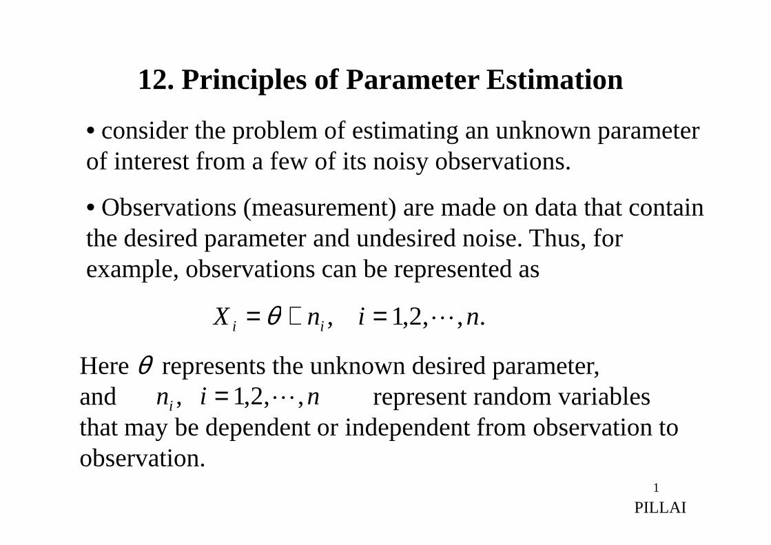
12. Principles of Parameter Estimation

• consider the problem of estimating an unknown parameter of interest from a few of its noisy observations.

• Observations (measurement) are made on data that contain the desired parameter and undesired noise. Thus, for example, observations can be represented as

1

example, observations can be represented as

PILLAI

.,,2,1 , ninX ii L=+= θ

Here θ represents the unknown desired parameter, and represent random variables that may be dependent or independent from observation to observation.

nini ,,2,1 , L=

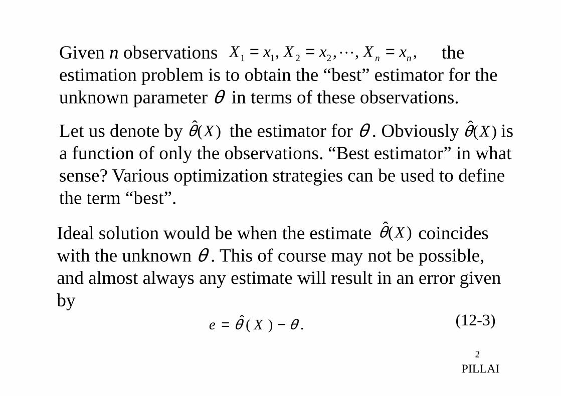
Given n observations the estimation problem is to obtain the “best” estimator for the unknown parameter θ in terms of these observations.

Let us denote by the estimator for θ . Obviously is a function of only the observations. “Best estimator” in what sense? Various optimization strategies can be used to define the term “best”.

, , , , 2211 nn xXxXxX === L

)(ˆ Xθ )(ˆ Xθ

2

the term “best”.

PILLAI

Ideal solution would be when the estimate coincides with the unknown θ . This of course may not be possible, and almost always any estimate will result in an error given by

(12-3).)(ˆ θθ −= Xe

)(ˆ Xθ

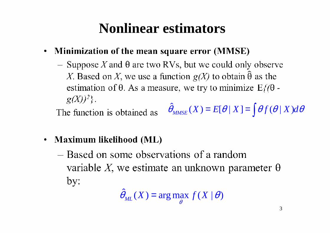
Nonlinear estimators

ˆ ( ) [ | ] ( | )MMSE X E X f X dθ θ θ θ θ= = ∫

3

∫

ˆ ( ) arg max ( | )ML X f Xθ

θ θ=

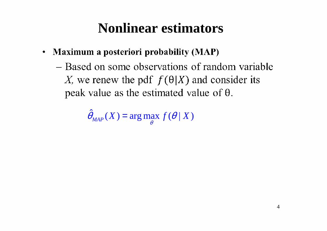
Nonlinear estimators

ˆ ( ) arg max ( | )X f Xθ θ=

4

ˆ ( ) arg max ( | )MAP X f Xθ

θ θ=

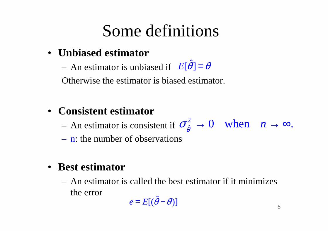
Some definitions• Unbiased estimator

– An estimator is unbiased if

Otherwise the estimator is biased estimator.

• Consistent estimator

ˆ[ ]E θ θ=

• Consistent estimator– An estimator is consistent if

– n: the number of observations

• Best estimator– An estimator is called the best estimator if it minimizes

the error

5

2ˆ 0 when .nθσ → → ∞

ˆ[( )]e E θ θ= −

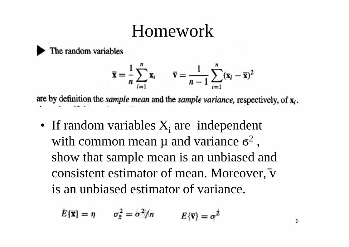
Homework

• If random variables Xare independent • If random variables Xi are independent with common mean µ and variance ϭ2 , show that sample mean is an unbiased and consistent estimator of mean. Moreover, ̄v is an unbiased estimator of variance.

6

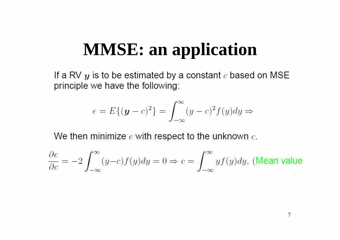
MMSE: an application

7

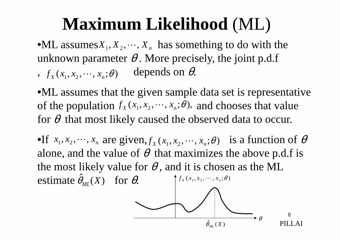
•ML assumes has something to do with the unknown parameter θ . More precisely, the joint p.d.f, depends on θ.

•ML assumes that the given sample data set is representative of the population and chooses that value for θ that most likely caused the observed data to occur.

nXXX , ,, 21 L

); , ,,( 21 θnX xxxf L

),; , ,,( 21 θnX xxxf L

Maximum Likelihood (ML)

8

for θ that most likely caused the observed data to occur.

•If are given, is a function of θalone, and the value of θ that maximizes the above p.d.f is the most likely value for θ , and it is chosen as the ML estimate for θ.

nxxx , ,, 21 L ); , ,,( 21 θnX xxxf L

)(ˆ XMLθ

)(ˆ XMLθ

); , ,,( 21 θnX xxxf L

θPILLAI

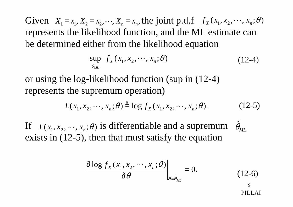
Given the joint p.d.frepresents the likelihood function, and the ML estimate can be determined either from the likelihood equation

or using the log-likelihood function (sup in (12-4) represents the supremumoperation)

, , , , 2211 nn xXxXxX === L ); , ,,( 21 θnX xxxf L

); , ,,( sup 21ˆ

θθ

nX xxxfML

L (12-4)

).; , ,,(log); , ,,( θθ xxxfxxxL LL = (12-5)∆

9

If is differentiable and a supremumexists in (12-5), then that must satisfy the equation

).; , ,,(log); , ,,( 2121 θθ nXn xxxfxxxL LL = (12-5)

); , ,,( 21 θnxxxL L

∆

MLθ̂

.0); , ,,(log

ˆ

21 =∂

∂

= ML

nX xxxf

θθθθL

(12-6)

PILLAI

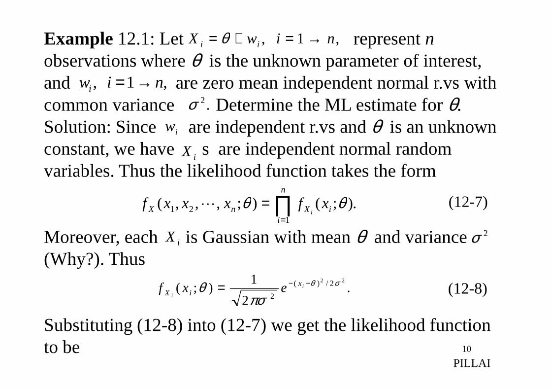
Example 12.1: Let represent nobservations where θ is the unknown parameter of interest, and are zero mean independent normal r.vs with common variance Determine the ML estimate for θ. Solution: Since are independent r.vs and θ is an unknown constant, we have s are independent normal random variables. Thus the likelihood function takes the form

,1 , niwX ii →=+= θ

.2σ,1 , niwi →=

iX

iw

.);(); , ,,( ∏=n

xfxxxf θθ (12-7)

10

Moreover, each is Gaussian with mean θ and variance (Why?). Thus

Substituting (12-8) into (12-7) we get the likelihood function to be

.);(); , ,,(1

21 ∏=

=i

iXnX xfxxxfi

θθL (12-7)

.2

1);(

22 2/)(

2

σθ

πσθ −−= i

i

xiX exf

iX 2σ

(12-8)

PILLAI

.)2(

1);,,,( 1

22 2/)(

2/221

∑= =

−−n

iix

nnX exxxfσθ

πσθL (12-9)

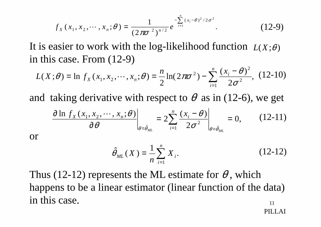
It is easier to work with the log-likelihood function in this case. From (12-9)

and taking derivative with respect to θ as in (12-6), we get

)(); , ,,(ln =−=∂∑

n xxxxf θθL

(12-10)

(12-11)

,2

)()2ln(

2);,,,(ln);(

12

22

21 ∑=

−−==n

i

inX

xnxxxfXL

σθπσθθ L

);( θXL

11

or

Thus (12-12) represents the ML estimate for θ , which happens to be a linear estimator (linear function of the data) in this case.

,02

)(2

); , ,,(ln

ˆ12

ˆ

21 =−=∂

∂

===∑

MLML

n

i

inX xxxxf

θθθθ σθ

θθL

.1

)(ˆ1∑

=

=n

iiML X

nXθ

(12-11)

(12-12)

PILLAI

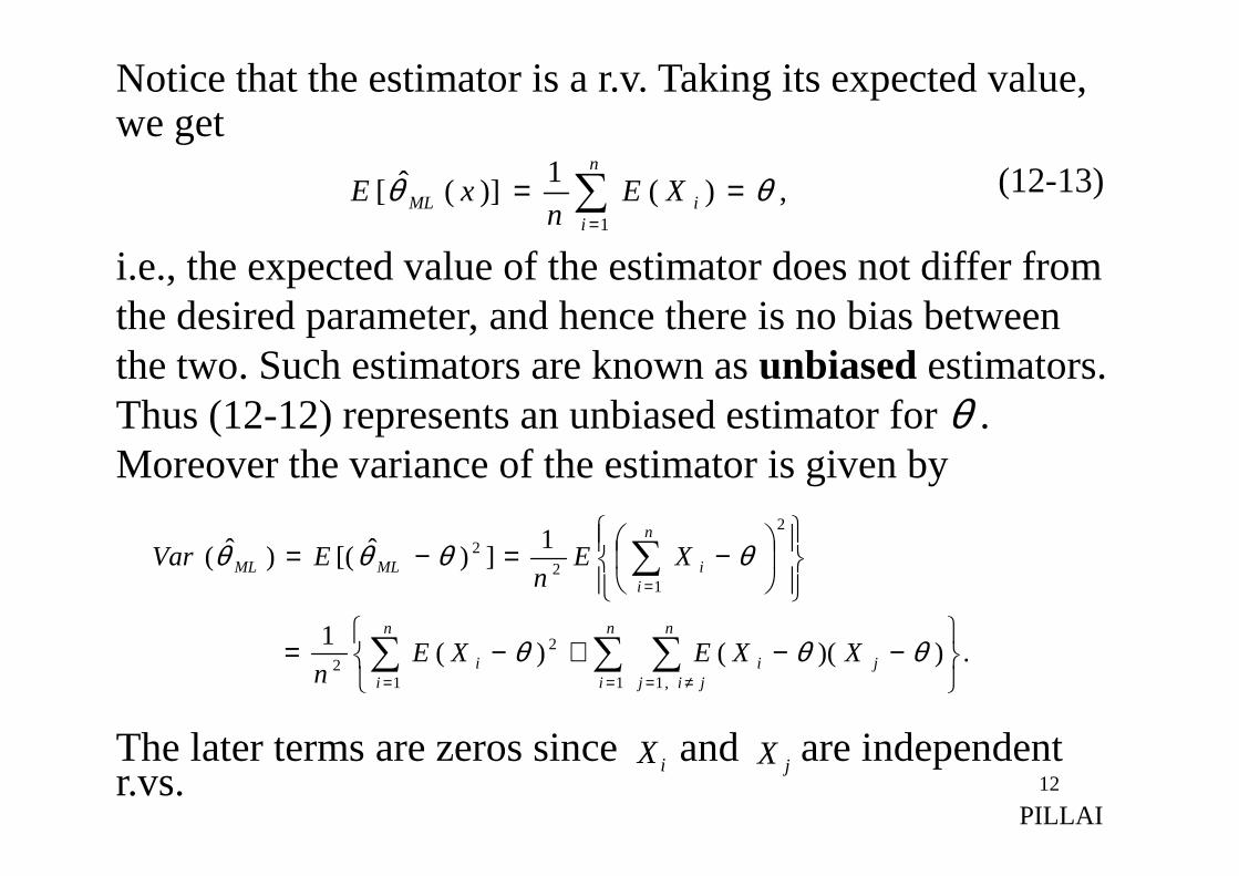
Notice that the estimator is a r.v. Taking its expected value, we get

i.e., the expected value of the estimator does not differ from the desired parameter, and hence there is no bias between the two. Such estimators are known as unbiased estimators. Thus (12-12) represents an unbiased estimator for θ .

,)(1

)](ˆ[1

θθ == ∑=

n

iiML XE

nxE (12-13)

12

Moreover the variance of the estimator is given by

The later terms are zeros since and are independent r.vs.

.))(()(1

1])ˆ[()ˆ(

1 ,11

22

2

12

2

−−+−=

−=−=

∑ ∑∑

∑

= ≠==

=

n

i

n

jijji

n

ii

n

iiMLML

XXEXEn

XEn

EVar

θθθ

θθθθ

iX jX

PILLAI

Then

Thus

another desired property. We say such estimators (that satisfy (12-15)) are consistent estimators.

(12-14).)(1

)ˆ(2

2

2

12 nn

nXVar

nVar

n

iiML

σσθ === ∑=

, as 0)ˆ( ∞→→ nVar MLθ (12-15)

13

Next two examples show that ML estimator can be highly nonlinear.

Example 12.2: Let be independent, identically distributed uniform random variables in the interval with common p.d.f

nXXX , ,, 21 L

),0( θ

,0 ,1

);( θθ

θ <<= iiX xxfi

PILLAI

(12-16)

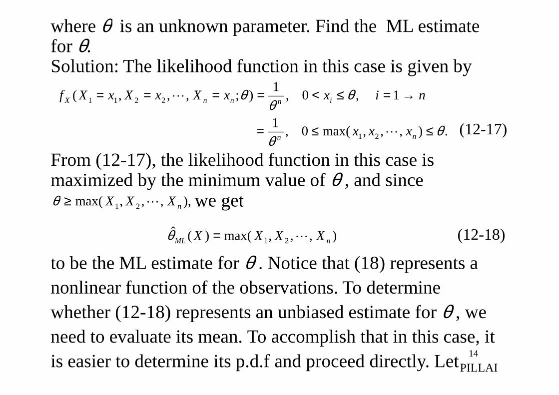
where θ is an unknown parameter. Find the ML estimate for θ. Solution: The likelihood function in this case is given by

From (12-17), the likelihood function in this case is maximized by the minimum value of θ , and since

we get

.) , ,,max(0 ,1

1 ,0 ,1

); , ,,(

21

2211

θθ

θθ

θ

≤≤=

→=≤<====

nn

innnX

xxx

nixxXxXxXf

L

L

(12-17)

), , ,,max( XXX L≥θ

14

we get

to be the ML estimate for θ . Notice that (18) represents a nonlinear function of the observations. To determine whether (12-18) represents an unbiased estimate for θ , we need to evaluate its mean. To accomplish that in this case, it is easier to determine its p.d.f and proceed directly. Let

), , ,,max( 21 nXXX L≥θ

) , ,,max()(ˆ21 nML XXXX L=θ (12-18)

PILLAI

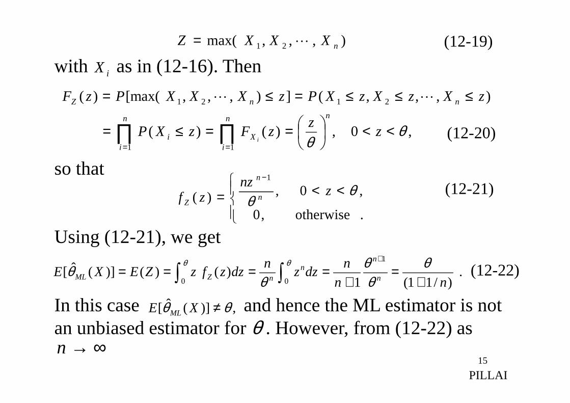
(12-19)) , ,,max( 21 nXXXZ L=

with as in (12-16). Then

so that

iX

,0 ,)()(

),,,(]) , ,,[max()(

11

2121

θθ

<<

==≤=

≤≤≤=≤=

∏∏==

zz

zFzXP

zXzXzXPzXXXPzFnn

iX

n

ii

nnZ

i

LL

(12-20)

,0 ,)(

1

<<=

−

θθ

znz

zf n

n

Z(12-21)

15

Using (12-21), we get

In this case and hence the ML estimator is not an unbiased estimator for θ . However, from (12-22) as

.otherwise,0

)(

= θzf nZ

. )/11(1

)( )()](ˆ[1

0

0 nn

ndzz

ndzzfzZEXE

n

nn

nZML +=

+====

+

∫∫θ

θθ

θθ

θθ(12-22)

,)](ˆ[ θθ ≠XE ML

∞→n

PILLAI

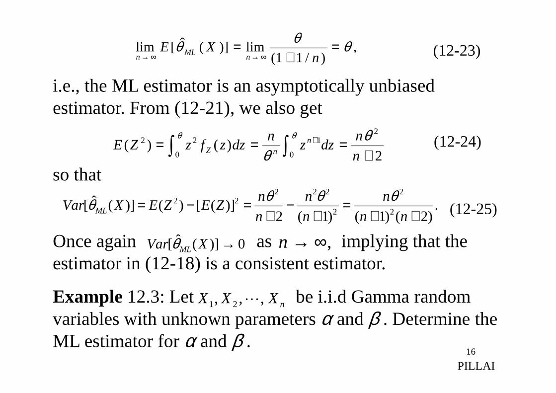
i.e., the ML estimator is an asymptotically unbiased estimator. From (12-21), we also get

so that

(12-23),)/11(

lim)](ˆ[lim θθθ =+

=∞→∞→ n

XEn

MLn

2)()(

2

0

1

0

22

+=== ∫∫

+

n

ndzz

ndzzfzZE n

nZ

θθ

θθ (12-24)

ˆ2222

22 =−=−= nnn θθθθ

16

Once again as implying that the estimator in (12-18) is a consistent estimator.

Example 12.3: Let be i.i.d Gamma random variables with unknown parameters α and β . Determine the ML estimator for α and β .

.)2()1()1(2

)]([)()](ˆ[22

22

++=

+−

+=−=

nn

n

n

n

n

nZEZEXVar ML

θθθθ

0)](ˆ[ →XVar MLθ ,∞→n

nXXX , ,, 21 L

PILLAI

(12-25)

Solution: Here and

This gives the log-likelihood function to be

Differentiating L with respect to α and β we get

,0≥ix

. ))((

),; , ,,(1

121

1∏=

−− ∑

Γ= =

n

i

x

in

n

nX

n

ii

exxxxfβ

αα

αββαL (12-26)

.log)1()(loglog

),; , ,,(log),; , ,,(

11

2121

∑∑==

−

−+Γ−=

=n

ii

n

ii

nXn

xxnn

xxxfxxxL

βααβα

βαβα LL

(12-27)

17

Differentiating L with respect to α and β we get

Thus from (12-29)

,0log)()(

logˆ,ˆ,1

=+Γ ′Γ

−=∂∂

==∑

βαβα

αα

βα

n

iix

nn

L (12-28)

.0ˆ,ˆ,1

=−=∂∂

==∑

βαβαβα

β

n

iix

nL(12-29)

,1

ˆ)(ˆ

1∑

=

=n

ii

MLML

xn

Xαβ (12-30)

PILLAI

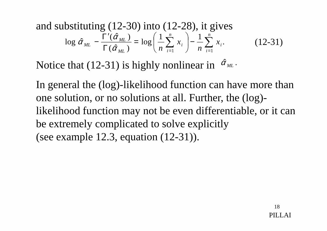
and substituting (12-30) into (12-28), it gives

Notice that (12-31) is highly nonlinear in

In general the (log)-likelihood function can have more than one solution, or no solutions at all. Further, the (log)-likelihood function may not be even differentiable, or it can

.11

log)ˆ(

)ˆ(ˆlog

11∑∑

==

−

=ΓΓ′

−n

ii

n

ii

ML

MLML x

nx

nααα

.ˆ MLα

(12-31)

18

likelihood function may not be even differentiable, or it can be extremely complicated to solve explicitly (see example 12.3, equation (12-31)).

PILLAI

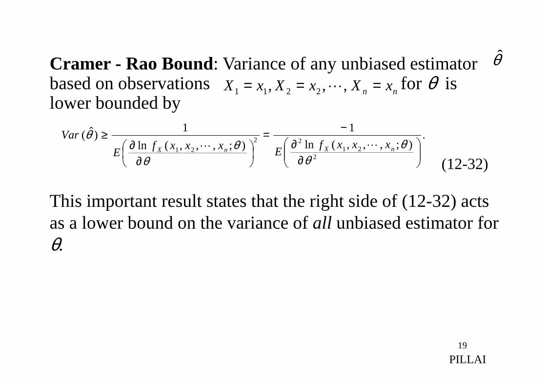
Cramer - Rao Bound: Variance of any unbiased estimator based on observations for θ is lower bounded by

This important result states that the right side of (12-32) acts

θ̂

nn xXxXxX === , ,, 2211 L

.

);,,,(ln

1

);,,,(ln

1)ˆ(

221

22

21

∂∂

−=

∂

∂≥

θθ

θθ

θnXnX xxxf

ExxxfE

VarLL

(12-32)

19

This important result states that the right side of (12-32) acts as a lower bound on the variance of all unbiased estimator for θ.

PILLAI

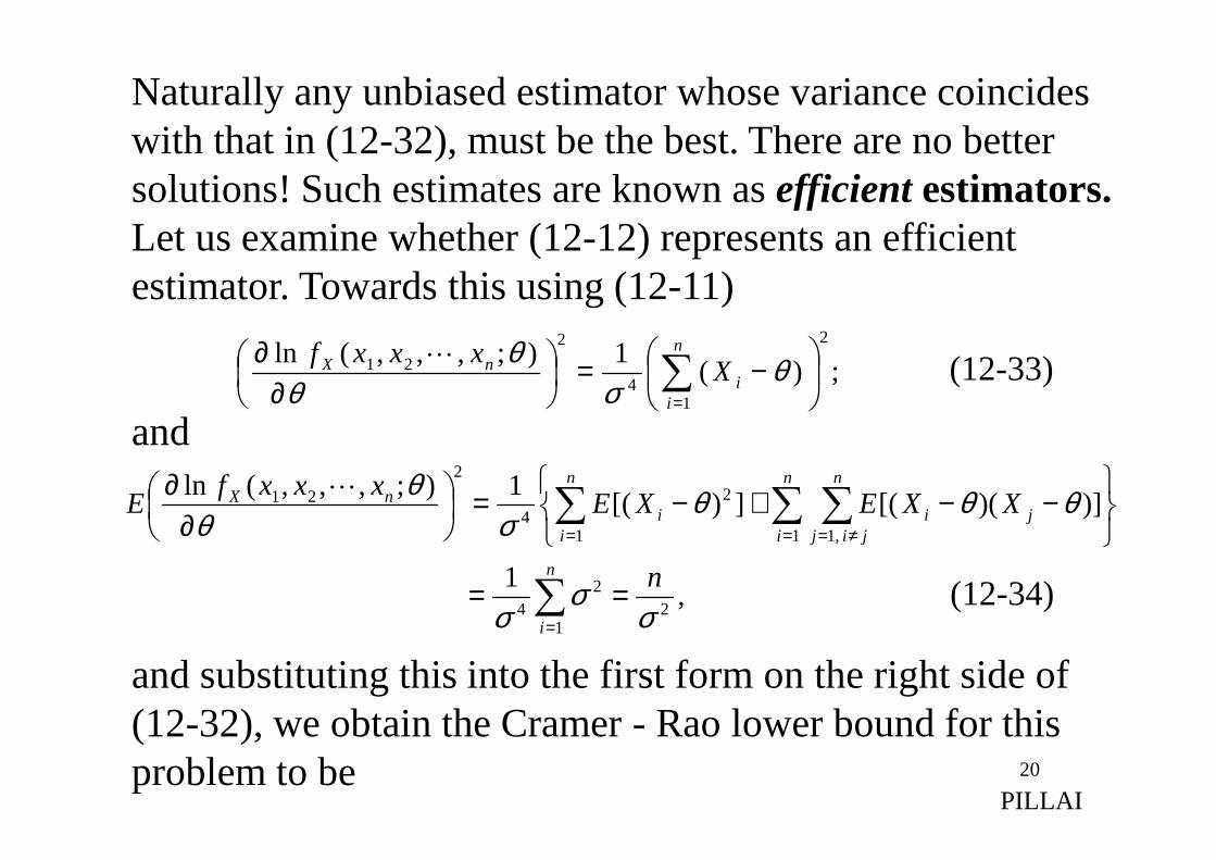
Naturally any unbiased estimator whose variance coincideswith that in (12-32), must be the best. There are no bettersolutions! Such estimates are known as efficient estimators.Let us examine whether (12-12) represents an efficient estimator. Towards this using (12-11)

and

;)(1

);,,,(ln2

14

2

21

−=

∂∂

∑=

n

ii

nX Xxxxf θ

σθθL (12-33)

20

and

and substituting this into the first form on the right side of(12-32), we obtain the Cramer - Rao lower bound for thisproblem to be

,1

)])([(])[(1

);,,,(ln

21

24

1 ,11

24

2

21

σσ

σ

θθθσθ

θ

n

XXEXExxxf

E

n

i

n

i

n

jijji

n

ii

nX

==

−−+−=

∂∂

∑

∑ ∑∑

=

= ≠==

L

(12-34)

PILLAI

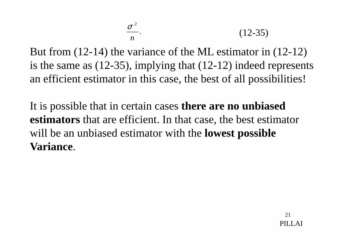
But from (12-14) the variance of the ML estimator in (12-12)is the same as (12-35), implying that (12-12) indeed representsan efficient estimator in this case, the best of all possibilities!

It is possible that in certain cases there are no unbiased estimators that are efficient. In that case, the best estimator

.2

n

σ(12-35)

21

PILLAI

estimators that are efficient. In that case, the best estimator will be an unbiased estimator with the lowest possible Variance.

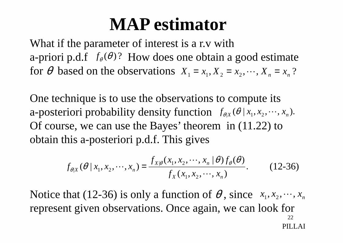
What if the parameter of interest is a r.v witha-priori p.d.f How does one obtain a good estimatefor θ based on the observations

One technique is to use the observations to compute itsa-posteriori probability density function Of course, we can use the Bayes’ theorem in (11.22) to

?)(θθf

? , ,, 2211 nn xXxXxX === L

). , ,,|( 21| nX xxxf Lθθ

MAP estimator

22

Of course, we can use the Bayes’ theorem in (11.22) toobtain this a-posteriori p.d.f. This gives

Notice that (12-36) is only a function of θ , since represent given observations. Once again, we can look for

.) , ,,(

)()| , ,,(), ,,|(

21

21|21|

nX

nXnX xxxf

fxxxfxxxf

L

LL

θθθ θθ

θ = (12-36)

nxxx , ,, 21 L

PILLAI

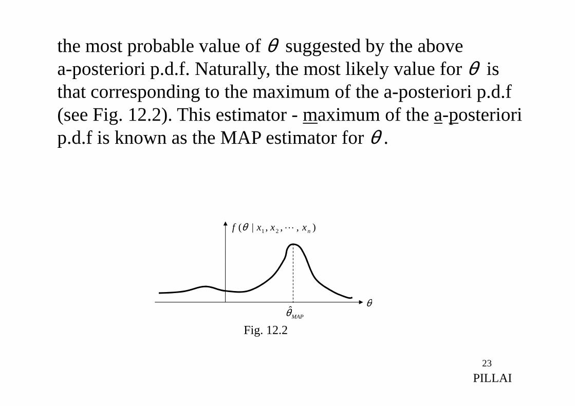
the most probable value of θ suggested by the abovea-posteriori p.d.f. Naturally, the most likely value for θ isthat corresponding to the maximum of the a-posteriori p.d.f(see Fig. 12.2). This estimator - maximum of the a-posteriorip.d.f is known as the MAP estimator for θ .

23

PILLAI

MAPθ̂

) , ,,|( 21 nxxxf Lθ

θ

Fig. 12.2