Lecture 11 STK3100/4100 - Summary

10. November 2014

– p. 1

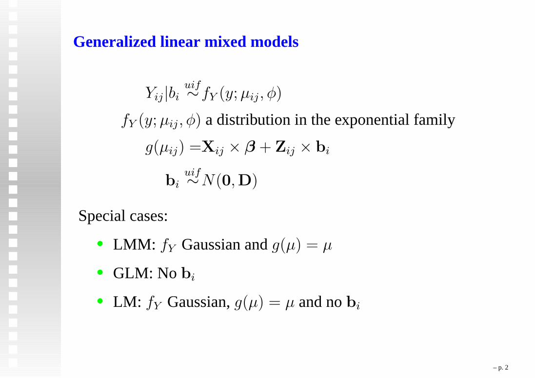
Generalized linear mixed models

Yij|biuif∼fY (y;µij, φ)

fY (y;µij, φ) a distribution in the exponential family

g(µij) =Xij × β + Zij × bi

biuif∼N(0,D)

Special cases:

• LMM: fY Gaussian andg(µ) = µ

• GLM: No bi

• LM: fY Gaussian,g(µ) = µ and nobi

– p. 2

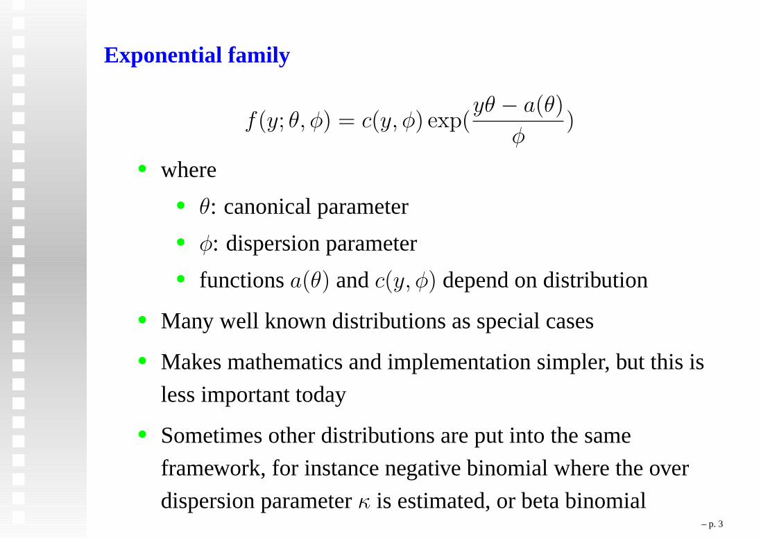
Exponential family

f(y; θ, φ) = c(y, φ) exp(yθ − a(θ)

φ)

• where

• θ: canonical parameter

• φ: dispersion parameter

• functionsa(θ) andc(y, φ) depend on distribution

• Many well known distributions as special cases

• Makes mathematics and implementation simpler, but this is

less important today

• Sometimes other distributions are put into the same

framework, for instance negative binomial where the over

dispersion parameterκ is estimated, or beta binomial– p. 3

G and M

• Generalized models allows

other distributions than the Gaussian and

link functions between expectation and linear predictor

• Mixed models allows dependencies between groups of

observations. Is an example ofhierarchical model model

– p. 4

Link functions

• Canonical link

• Gives simpler mathematics and estimation algorithms

• Not very important today, use the link functions that

fits your problem

• Different alternative link functions for various models, for

instance logit, probit and complementary log-log for

binomial distribution, power link for Poisson

– p. 5

Steps in analysis by GLM and GLMM

• Choose distribution for response variable

• Choose link function

• Estimation and inference for given model

• Model selection

• Choose structure for random effects (GLMM)

• Choose structure for fixed effects

• Model validation

• Prediction

– p. 6

Estimation

• General principle: Maximum likelihood (ML)

• Random effects: ML can underestimate variances, REML

is an alternative, but in practice only for LMM, not GLMM

• PQL a simpler alternative to ML for GLMM

– p. 7

Numerical methods

• GLM: Newton-Raphson/Fisher scoring OK

• LMM: Likelihood directly available

• Likelihood can be optimised by numerical methods,

(but we have not discussed such methods in the course)

• GLMM: Likelihood more difficult to compute

• Simpler criterion: PQL

• Numerical approximations (Laplace, Gauss-Hermite)

– p. 8

Properties of ML estimates

• Good large sample properties

• Consistent

• Asymptotically normal distributed

• Covariance matrix given by the inverse Fisher information

matrix

• Some problems for variances

• Biased

• Boundary effects

– p. 9

Interpretation of parameters

• Depends on link function

• We have studied this for link functions used in Poisson and

binomial regression

• Poisson with log link:exp(β) is rate ratio

• Binomial with logit link: exp(β) is odds ratio

• In models with random effects: Parameters directly

interpretable on individual level

• LMM: Same interpretation on population level

– p. 10

Offset i models for counts

µi = ni exp(β0 +∑

j

βjxij)

= exp(β0 + log(ni) +∑

j

βjxij)

log(µi) = β0 + 1 · log(ni) +∑

j

βjxij

– p. 11

Sensitivity and specificity in models for binary response

• Sensitivity: Proportion of correct predictions when true

Yi = 1

• Specificity: Proportion of correct predictions when true

Yi = 0

• ROC curve: Plot sensitivity vs. (1-specificy) for varying

values of the classification thresholds

– p. 12

Continuous positive responses

• Lognormal

• Gamma

• Inverse Gaussian

– p. 13

Over dispersion and variance structure

• Each distribution within the exponential family has a

variance structure on the form Var[Yij] = φV (µij)

• Poisson/binomial:φ = 1

• Over dispersion if data indicatesφ > 1

• Possibility 1: Quasi likelihood, only specify mean

and variance structure, not a distribution• Possibility 2 Poisson: Use negative binomial

distribution - Var(Yi) = µi + θµ2i

• Possibility 2 “binomial”: Use beta binomial

distribution - Var(Yi) = (1 + ρ(ni − 1))niπ(1− π))

• Mixed models with random intercept

– p. 14

Model selection

Various methods:

• Likelihood ratio test/deviance test

• Wald z/t test,χ2/F test

• Wald z, χ2 if known dispersion parameter

• Wald t, F if unknown dispersion parameter

• AIC/BIC

Which method that is most appropriate depends on

• Type of model

• Which part of model one want to test

– p. 15

Model selection protocol for LMM

Main idea: Want to explain as much as possible by fixed effects

1. Start with a large model with as many explanatory variables

and interactions as possible

2. Find optimal structure on random effects using REML

3. Find optimal structure for fixed effects using both ML

(LRT) and REML (t/F-tests)

4. Estimate the final model using REML

– p. 16

Likelihood ratio test

• General method, can be used to test both fixed and random

effects

• The models to be compared have to benested

• Fixed effects: Use ML

• Random effects: Use REML (for LMM)

Boundary effects: Mixture ofχ2v andχ2

v−1 distribution

• One-to-one correspondence to deviance differences

– p. 17

Wald test

• Useful to test fixed effects

• If dispersion parameter known: use normal distribution

• If dispersion parameter unknown: uset distribution

• Can be generalised to more than one parameter (factors

with more than tho levels), givesχ2/F distribution

• Simpler than LRT, do only need to fit one model

• Worse small sample properties than LRT

– p. 18

AIC/BIC

• Optimise likelihood with penalty for model complexity

• AIC: - 2 log likelihood + 2p

• BIC: - 2 log likelihood + log(n) p

• Can be used to compare both nested and non-nested models

• For LMM:

• For fixed effects: Use ML

• For random effects: Use REML

– p. 19

Number of parameters in LMM and GLMM

• The book and the R software use

p = number of fixed effects

+ number of variance parameters

• Could instead useeffective number of parameters, but this

is difficult to calculate

• Still a research field

– p. 20

Residuals

• Useful for model validation

• Different versions

• Response residualsyij − yij

• Pearson residuals:rPi =Yi−µi

Var(Yi)0.5

• Deviance residuals:r∆i = sign(Yi − µi)

√2(li − li)

• Anscombe residuals

• For mixed models:yij can be computed at different levels

• Most useful to study residualswithin groups

– p. 21

Model validation

• Residual plots

• Distribution of residuals

• Residuals vs. fitted values

• Deviance test

• Comparison with saturated model

• Residual deviance should be small compared to

number of degrees of freedom

• Useful for models with known dispersion parameter

and expected number of observations

within each cell> 5

• Hosmer-Lemeshow test alternative for binomial regression

– p. 22

Prediction

• LMM and GLMM: Can be done at different levels

• Level 0: µij = g−1(Xij × β)

• Level 1: µij = g−1(Xij × β + Zij × bi)

bi = E[bi|Y, β, θ]

– p. 23

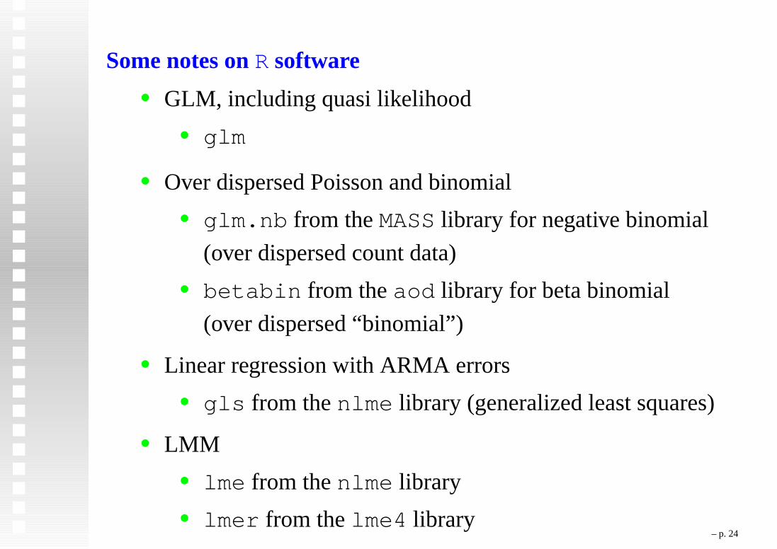
Some notes onR software

• GLM, including quasi likelihood

• glm

• Over dispersed Poisson and binomial

• glm.nb from theMASS library for negative binomial

(over dispersed count data)

• betabin from theaod library for beta binomial

(over dispersed “binomial”)

• Linear regression with ARMA errors

• gls from thenlme library (generalized least squares)

• LMM

• lme from thenlme library

• lmer from thelme4 library– p. 24

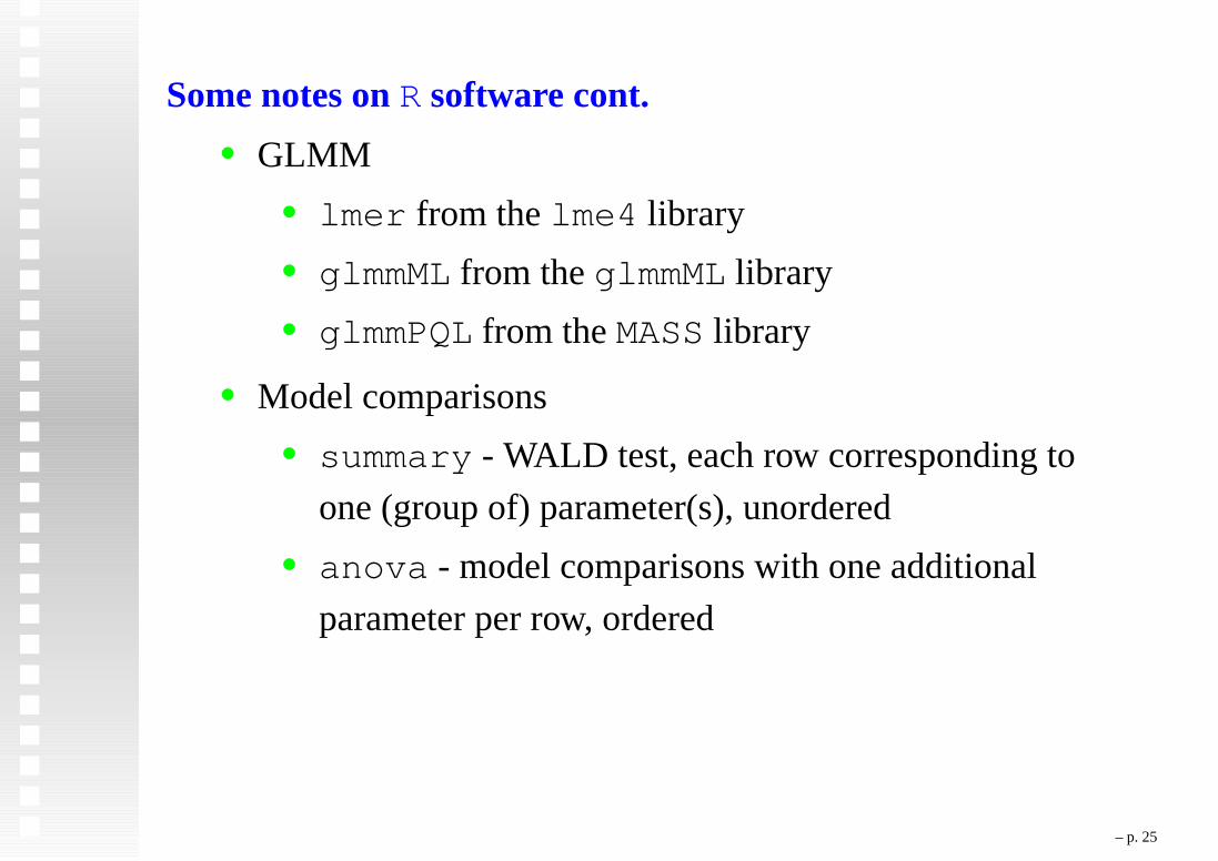
Some notes onR software cont.

• GLMM

• lmer from thelme4 library

• glmmML from theglmmML library

• glmmPQL from theMASS library

• Model comparisons

• summary - WALD test, each row corresponding to

one (group of) parameter(s), unordered

• anova - model comparisons with one additional

parameter per row, ordered

– p. 25

Syllabus

See the course web page

– p. 26