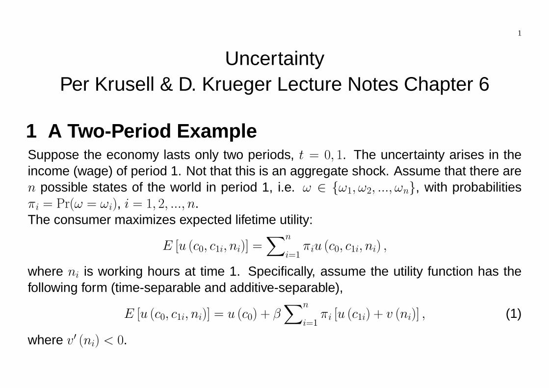
1

UncertaintyPer Krusell & D. Krueger Lecture Notes Chapter 6

1 A Two-Period ExampleSuppose the economy lasts only two periods, t = 0, 1. The uncertainty arises in theincome (wage) of period 1. Not that this is an aggregate shock. Assume that there aren possible states of the world in period 1, i.e. ω ∈ {ω1, ω2, ..., ωn}, with probabilitiesπi = Pr(ω = ωi), i = 1, 2, ..., n.The consumer maximizes expected lifetime utility:

E [u (c0, c1i, ni)] =Xn

i=1πiu (c0, c1i, ni) ,

where ni is working hours at time 1. Specifically, assume the utility function has thefollowing form (time-separable and additive-separable),

E [u (c0, c1i, ni)] = u (c0) + βXn

i=1πi [u (c1i) + v (ni)] , (1)

where v0 (ni) < 0.

2

1.1 A Risk-free AssetThere is a “risk free” asset (similar to a storage technology) denoted by a, which ispriced q at time 0, such that every unit of a purchased in period 0 pays 1 unit of goods inperiod 1, regardless of the state of the world. The consumer faces the following budgetrestriction in period 0, given a fixed time 0 income I:

c0 + aq = I. (2)

At each realization of the state of the world, his budget constraint in period 1 is

c1i = a + wini, i = 1, ..., n. (3)

The consumer’s problem is to choose (c0, a, {c1i, ni}ni=1) to maximize (1), subject to (2)and (3). The Lagrangian is

L = u (I − aq) + βXn

i=1πi [u (c1i) + v (ni)] +

Xn

i=1λi (a+ wini − c1i) .

3

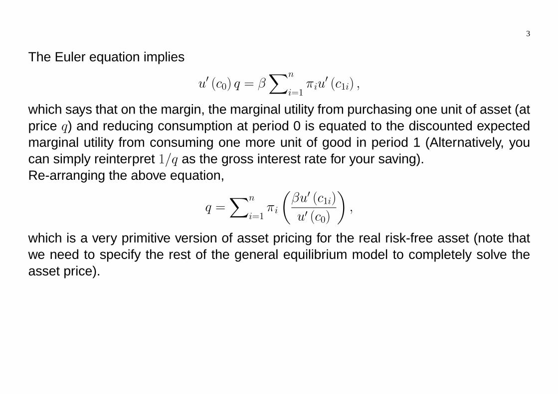
The Euler equation implies

u0 (c0) q = βXn

i=1πiu

0 (c1i) ,

which says that on the margin, the marginal utility from purchasing one unit of asset (atprice q) and reducing consumption at period 0 is equated to the discounted expectedmarginal utility from consuming one more unit of good in period 1 (Alternatively, youcan simply reinterpret 1/q as the gross interest rate for your saving).Re-arranging the above equation,

q =Xn

i=1πi

µβu0 (c1i)

u0 (c0)

¶,

which is a very primitive version of asset pricing for the real risk-free asset (note thatwe need to specify the rest of the general equilibrium model to completely solve theasset price).

4

Example: Let u(c) = c1−σ−11−σ , where σ is the coefficient of relative risk aversion and is

the inverse of the elasticity of intertemporal substitution (the higher σ, the less willingthe consumer is to experience the fluctuations of consumption over time). let σ = 1,then u(c) = ln(c). We also assume v(n) = ln(1 − n). Using the FOCs and the budgetconstraint at state i, we have

c1i =a + wi

2.

Note that there is no state-contingent transfer of wealth in the period 1, and thus period1 consumption may fluctuate a lot, depending on the realization of wi. The holding ofasset a can be solved, again by FOCs and the budget constraints,

q

I − aq= β

Xn

i=1πi

2

a + wi.

Normalizing the supply of the asset to be unity, then a = 1 in equilibrium, and we cansolve for the asset price from this equation.

5

1.2 Arrow SecuritiesInstead of a risk-free asset yielding the same payout in each state, we consider “Arrowsecurities” (state-contingent claims): n assets are traded in period 0 (each priced qi),and each unit of asset i purchased pays off 1 unit if the realized state is i, and 0otherwise.The budget constraint in period 0 is

c0 +Xn

i=1qiai = I. (4)

At each realization of the state of the world, his budget constraint in period 1 is

c1i = ai + wini, i = 1, ..., n. (5)

Will the consumer be better with this market structure?The market structure now allows the wealth transfer across periods to be state-specific:not only can the consumer reallocate his income between periods 0 and 1, but alsomove his wealth across states of the world.

6

Replacing ai, the (intertemporal) budget constraint becomes

c0 +Xn

i=1qic1i = I +

Xn

i=1qiwini.

The Euler equation implies

u0 (c0) qi = βπiu0 (c1i) .

Note that the Euler equation holds for every realization of the state of the world. Alsothe asset price i depends on the MRS of between consumption in period 0 and con-sumption in period 1 when state i occurs,

qi =βπiu

0 (c1i)

u0 (c0)≡MRS(c1i, c0).

If MRS(c1i, c0) is large, i.e., in order to increase one unit of date 1 good in state i, theconsumer is willing to give up a large amount of date 0 good, and thus the consumeris willing to pay a high price for the security.The relative asset price across state equals to the marginal rates of substitution across

7

statesqiqj=

βπiu0 (c1i)

βπju0 (c1j)≡MRS(c1i, c1j).

Example: Given log utility function, the availability of Arrow securities implies

c1i =βπiqi

c0,

which says that consumption in each state is proportional to consumption in period 0,c0 and is independent of the realization of wi. This proportionality is a function of thecost of insurance: the higher qi (the consumer is willing to pay a higher price for thesecurity i) in relation to πi, the lower the wealth transfer into state i. In this way, agentsare able to diversify risk efficiently.

8

2 Representation of Uncertainty

We start with the notion of an event st. The realizations st are drawn from a set S:st ∈ S, ∀t. The set S = {η1, , ..., ηN} of possible events is assumed to be finite and thesame for all periods t. In the following, we use the notation st = 1 instead of st = η1and so forth.An event history st = (st, st−1, ..., s0) is a vector of length t + 1 keeping track of therealizations of all events up from period 0 to period t. Notice that s0 = s0, and we canwrite st =

¡st, s

t−1¢.Formally, St = S × S... × S denoting the t + 1-fold product of S, event history st ∈ St

lies in the set of all possible event histories.Let π (st) denote the probability of a particular event history. Assume that π (st) ≥ 0 forall st ∈ St, for all t.

9

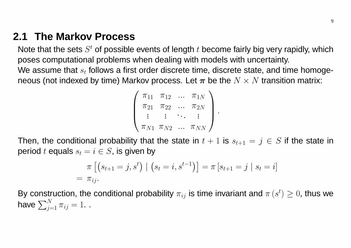
2.1 The Markov ProcessNote that the sets St of possible events of length t become fairly big very rapidly, whichposes computational problems when dealing with models with uncertainty.We assume that st follows a first order discrete time, discrete state, and time homoge-neous (not indexed by time) Markov process. Let π be the N ×N transition matrix:⎛⎜⎜⎝

π11 π12 ... π1Nπ21 π22 ... π2N... ... . . . ...

πN1 πN2 ... πNN

⎞⎟⎟⎠ .

Then, the conditional probability that the state in t + 1 is st+1 = j ∈ S if the state inperiod t equals st = i ∈ S, is given by

㜭st+1 = j, st

¢|¡st = i, st−1

¢¤= π [st+1 = j | st = i]

= πij.

By construction, the conditional probability πij is time invariant and π (st) ≥ 0, thus wehave

PNj=1 πij = 1. .

10

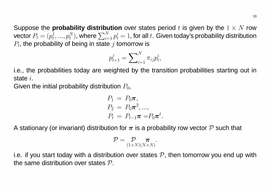
Suppose the probability distribution over states period t is given by the 1 × N rowvector Pt = (p

1t , ..., p

Nt ), where

PNi=1 p

it = 1, for all t. Given today’s probability distribution

Pt, the probability of being in state j tomorrow is

pjt+1 =XN

i=1πijp

it,

i.e., the probabilities today are weighted by the transition probabilities starting out instate i.Given the initial probability distribution P0,

P1 = P0π,

P2 = P0π2, ...,

Pt = Pt−1π =P0πt.

A stationary (or invariant) distribution for π is a probability row vector P such that

P = P(1×N)

π(N×N)

.

i.e. if you start today with a distribution over states P, then tomorrow you end up withthe same distribution over states P.

11

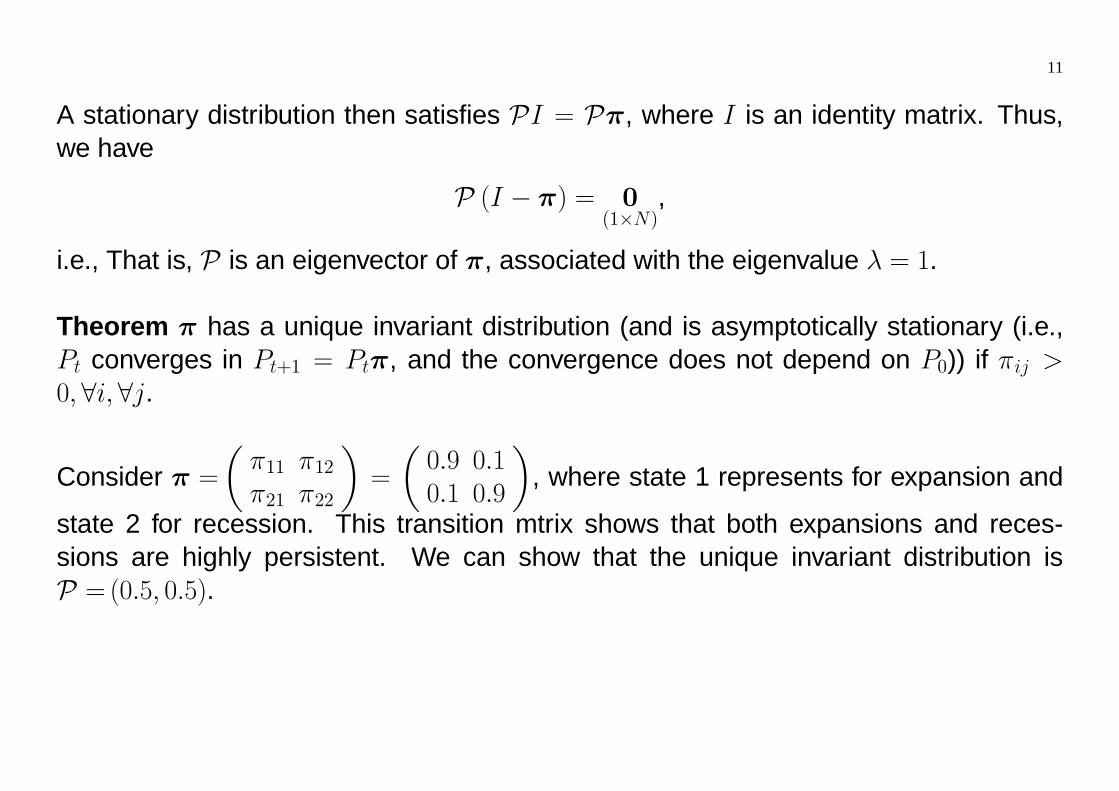
A stationary distribution then satisfies PI = Pπ, where I is an identity matrix. Thus,we have

P (I − π) = 0(1×N)

,

i.e., That is, P is an eigenvector of π, associated with the eigenvalue λ = 1.

Theorem π has a unique invariant distribution (and is asymptotically stationary (i.e.,Pt converges in Pt+1 = Ptπ, and the convergence does not depend on P0)) if πij >0,∀i,∀j.

Consider π =µπ11 π12π21 π22

¶=

µ0.9 0.10.1 0.9

¶, where state 1 represents for expansion and

state 2 for recession. This transition mtrix shows that both expansions and reces-sions are highly persistent. We can show that the unique invariant distribution isP =(0.5, 0.5).

12

3 The Stochastic Neoclassical Growth Model

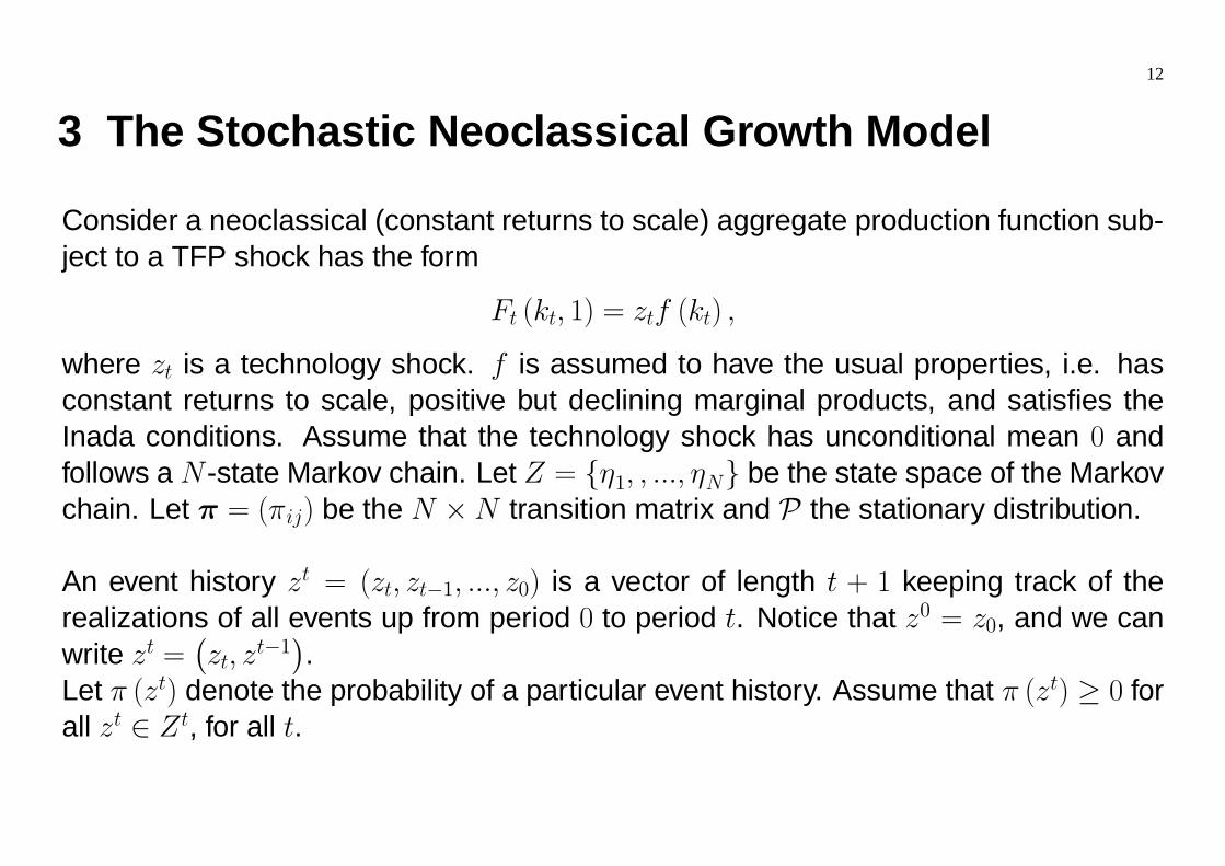
Consider a neoclassical (constant returns to scale) aggregate production function sub-ject to a TFP shock has the form

Ft (kt, 1) = ztf (kt) ,

where zt is a technology shock. f is assumed to have the usual properties, i.e. hasconstant returns to scale, positive but declining marginal products, and satisfies theInada conditions. Assume that the technology shock has unconditional mean 0 andfollows a N -state Markov chain. Let Z = {η1, , ..., ηN} be the state space of the Markovchain. Let π = (πij) be the N ×N transition matrix and P the stationary distribution.

An event history zt = (zt, zt−1, ..., z0) is a vector of length t + 1 keeping track of therealizations of all events up from period 0 to period t. Notice that z0 = z0, and we canwrite zt =

¡zt, z

t−1¢.Let π (zt) denote the probability of a particular event history. Assume that π (zt) ≥ 0 forall zt ∈ Zt, for all t.

13

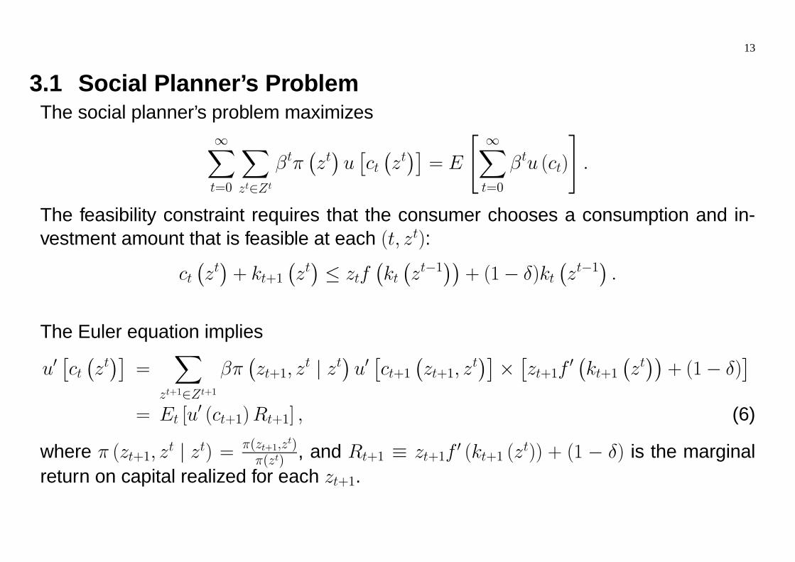
3.1 Social Planner’s ProblemThe social planner’s problem maximizes

∞Xt=0

Xzt∈Zt

βtπ¡zt¢u£ct¡zt¢¤= E

" ∞Xt=0

βtu (ct)

#.

The feasibility constraint requires that the consumer chooses a consumption and in-vestment amount that is feasible at each (t, zt):

ct¡zt¢+ kt+1

¡zt¢≤ ztf

¡kt¡zt−1

¢¢+ (1− δ)kt

¡zt−1

¢.

The Euler equation implies

u0£ct¡zt¢¤=

Xzt+1∈Zt+1

βπ¡zt+1, z

t | zt¢u0£ct+1

¡zt+1, z

t¢¤×£zt+1f

0 ¡kt+1 ¡zt¢¢ + (1− δ)¤

= Et [u0 (ct+1)Rt+1] , (6)

where π (zt+1, zt | zt) = π(zt+1,z

t)π(zt) , and Rt+1 ≡ zt+1f

0 (kt+1 (zt)) + (1 − δ) is the marginal

return on capital realized for each zt+1.

14

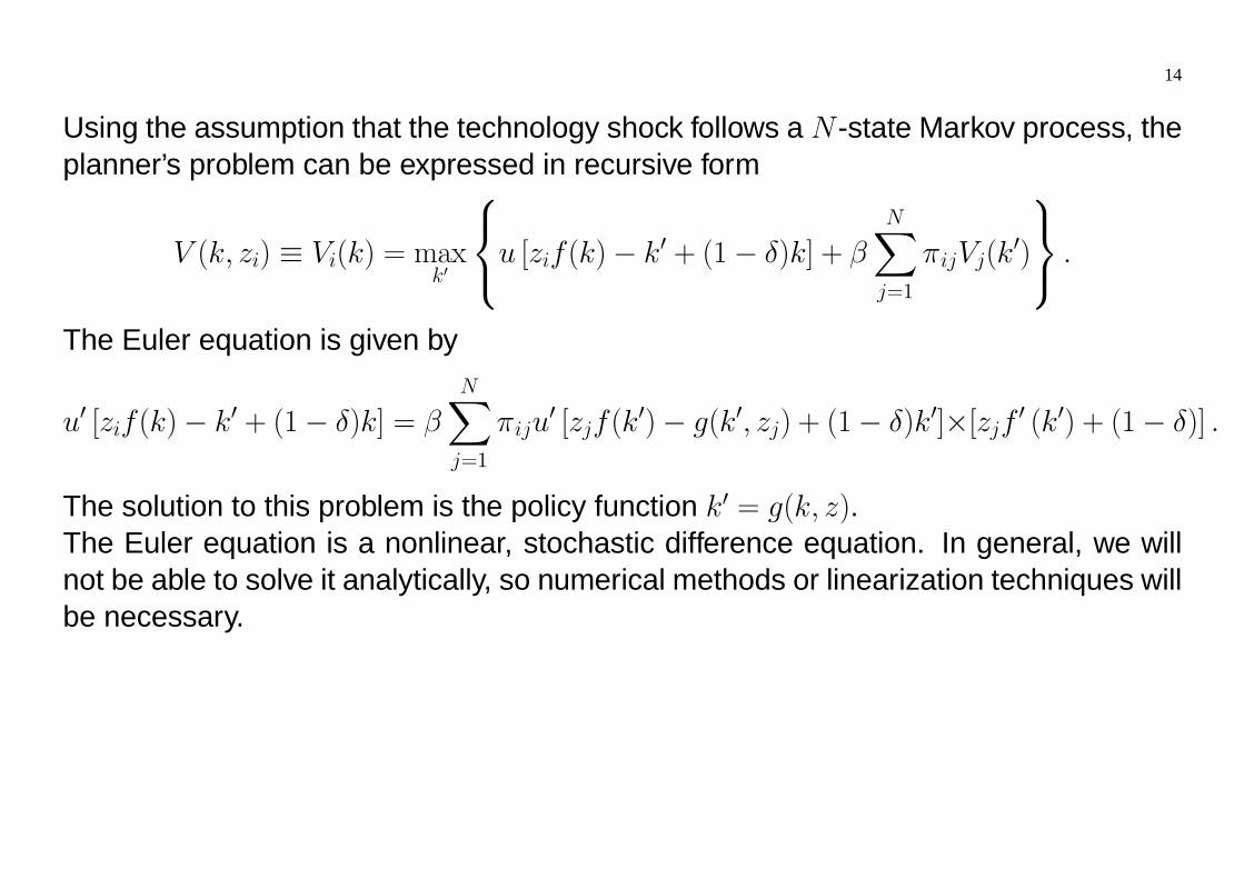
Using the assumption that the technology shock follows a N -state Markov process, theplanner’s problem can be expressed in recursive form

V (k, zi) ≡ Vi(k) = maxk0

⎧⎨⎩u [zif(k)− k0 + (1− δ)k] + βNXj=1

πijVj(k0)

⎫⎬⎭ .

The Euler equation is given by

u0 [zif(k)− k0 + (1− δ)k] = βNXj=1

πiju0 [zjf(k

0)− g(k0, zj) + (1− δ)k0]×[zjf 0 (k0) + (1− δ)] .

The solution to this problem is the policy function k0 = g(k, z).The Euler equation is a nonlinear, stochastic difference equation. In general, we willnot be able to solve it analytically, so numerical methods or linearization techniques willbe necessary.

15

3.2 Competitive equilibrium

In the social planner’s problem, the planner allocates {ct (zt) , kt+1 (zt)} according tothe history of states zt. Note that a commodity with a particular history of realizationsof the random sequence ct (z

t) is a commodity different from ct (zt) resulting from an-

other history of realizations of the random sequence. How to implement these statecontingent commodities?

A complete markets structure will allow contracts between parties to specify and en-force the delivery of physical good in different amounts for different realizations of therandom sequence for a different price. The Arrow-Debreu economy specifies the fullset of state contingent commodities at date 0 and assumes that these contracts can beperfectly enforced.

16

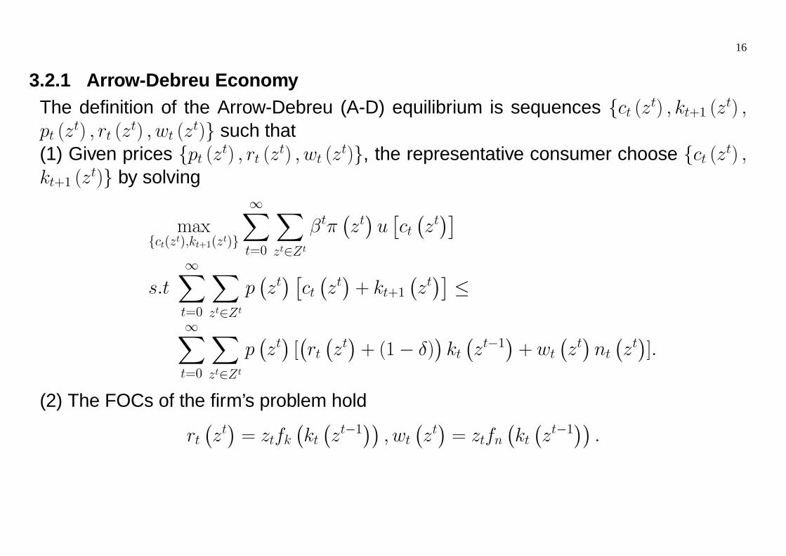
3.2.1 Arrow-Debreu EconomyThe definition of the Arrow-Debreu (A-D) equilibrium is sequences {ct (zt) , kt+1 (zt) ,pt (z

t) , rt (zt) , wt (z

t)} such that(1) Given prices {pt (zt) , rt (zt) , wt (z

t)}, the representative consumer choose {ct (zt) ,kt+1 (z

t)} by solving

max{ct(zt),kt+1(zt)}

∞Xt=0

Xzt∈Zt

βtπ¡zt¢u£ct¡zt¢¤

s.t∞Xt=0

Xzt∈Zt

p¡zt¢ £ct¡zt¢+ kt+1

¡zt¢¤≤

∞Xt=0

Xzt∈Zt

p¡zt¢[¡rt¡zt¢+ (1− δ)

¢kt¡zt−1

¢+ wt

¡zt¢nt¡zt¢].

(2) The FOCs of the firm’s problem hold

rt¡zt¢= ztfk

¡kt¡zt−1

¢¢, wt

¡zt¢= ztfn

¡kt¡zt−1

¢¢.

17

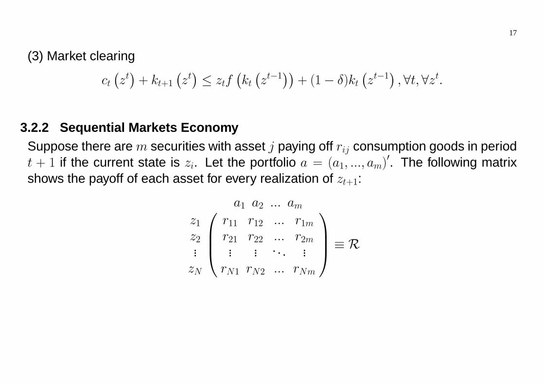
(3) Market clearing

ct¡zt¢+ kt+1

¡zt¢≤ ztf

¡kt¡zt−1

¢¢+ (1− δ)kt

¡zt−1

¢,∀t,∀zt.

3.2.2 Sequential Markets EconomySuppose there are m securities with asset j paying off rij consumption goods in periodt + 1 if the current state is zi. Let the portfolio a = (a1, ..., am)

0. The following matrixshows the payoff of each asset for every realization of zt+1:

z1z2...zN

a1 a2 ... am⎛⎜⎜⎝r11 r12 ... r1mr21 r22 ... r2m... ... . . . ...

rN1 rN2 ... rNm

⎞⎟⎟⎠ ≡ R

18

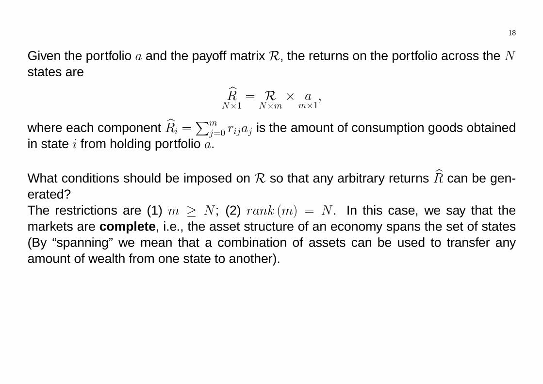
Given the portfolio a and the payoff matrix R, the returns on the portfolio across the Nstates are bR

N×1= R

N×m× a

m×1,

where each component bRi =Pm

j=0 rijaj is the amount of consumption goods obtainedin state i from holding portfolio a.

What conditions should be imposed on R so that any arbitrary returns bR can be gen-erated?The restrictions are (1) m ≥ N ; (2) rank (m) = N . In this case, we say that themarkets are complete, i.e., the asset structure of an economy spans the set of states(By “spanning” we mean that a combination of assets can be used to transfer anyamount of wealth from one state to another).

19

Recall that Arrow security i pays off 1 unit of good if the realized state is i, and 0otherwise. Since each Arrow security is linearly independent, N Arrow securities willbe able to span the entire state returns space. In this case, the markets are complete.

If rank (m) < N , i.e. the number of linearly independent securities is less than thenumber of states, then the set of assets does not “span” the entire state returns spaceand we will have incomplete markets. In this case, Pareto optimality will be in generalnot achievable.

20

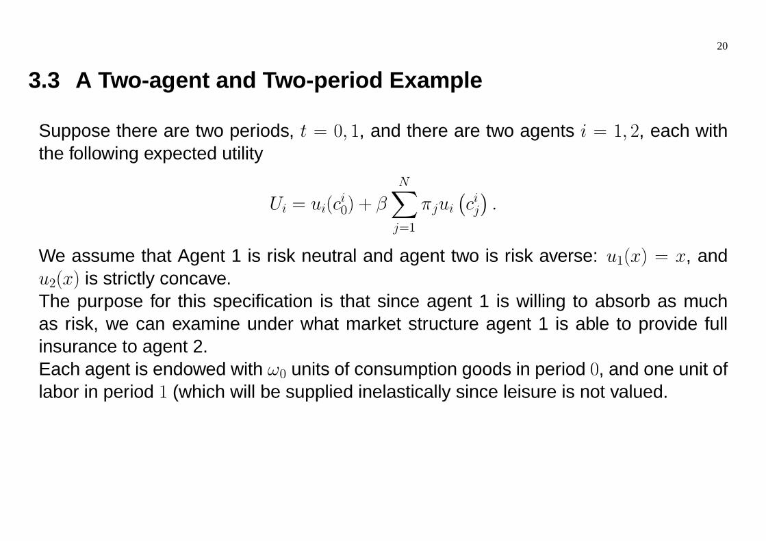
3.3 A Two-agent and Two-period Example

Suppose there are two periods, t = 0, 1, and there are two agents i = 1, 2, each withthe following expected utility

Ui = ui(ci0) + β

NXj=1

πjui¡cij¢.

We assume that Agent 1 is risk neutral and agent two is risk averse: u1(x) = x, andu2(x) is strictly concave.The purpose for this specification is that since agent 1 is willing to absorb as muchas risk, we can examine under what market structure agent 1 is able to provide fullinsurance to agent 2.Each agent is endowed with ω0 units of consumption goods in period 0, and one unit oflabor in period 1 (which will be supplied inelastically since leisure is not valued.

21

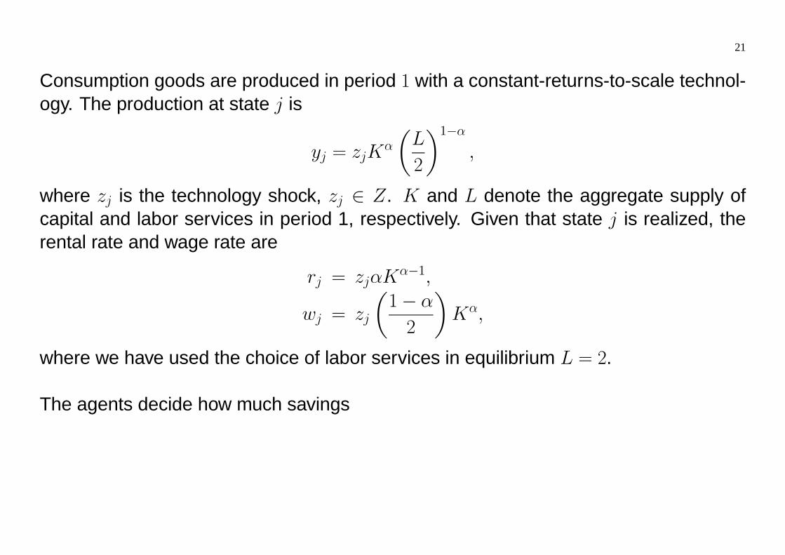
Consumption goods are produced in period 1 with a constant-returns-to-scale technol-ogy. The production at state j is

yj = zjKα

µL

2

¶1−α,

where zj is the technology shock, zj ∈ Z. K and L denote the aggregate supply ofcapital and labor services in period 1, respectively. Given that state j is realized, therental rate and wage rate are

rj = zjαKα−1,

wj = zj

µ1− α

2

¶Kα,

where we have used the choice of labor services in equilibrium L = 2.

The agents decide how much savings

22

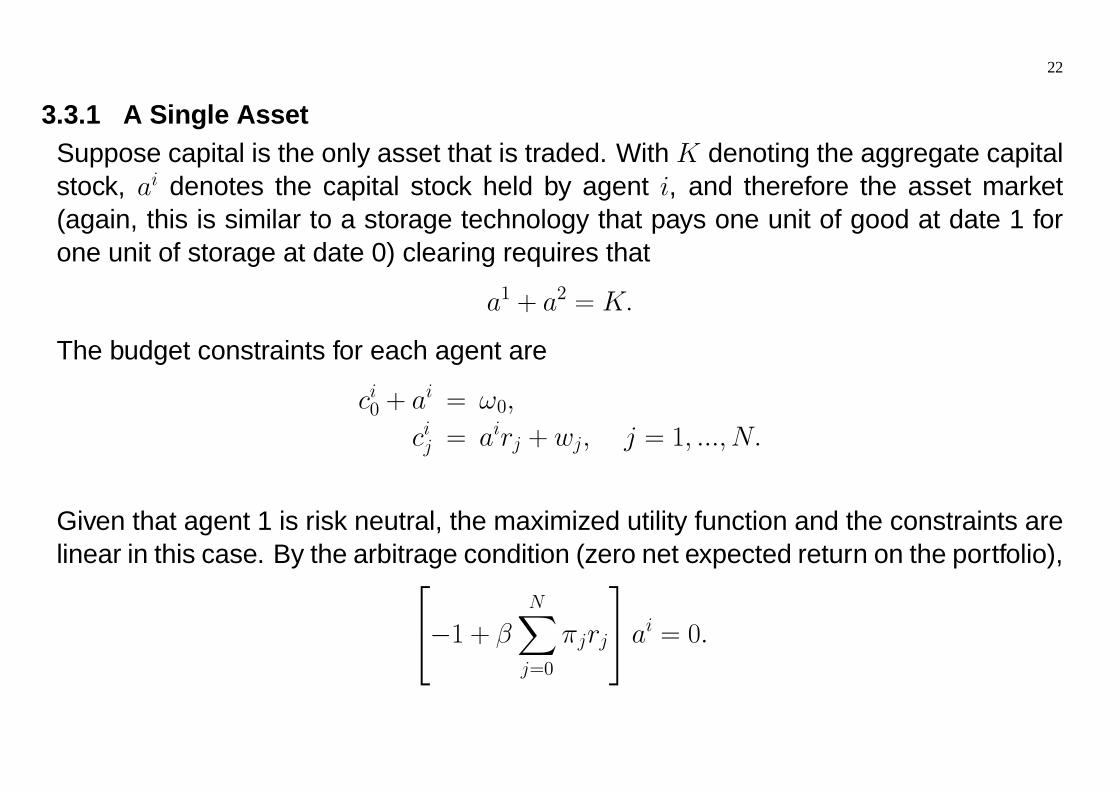
3.3.1 A Single AssetSuppose capital is the only asset that is traded. With K denoting the aggregate capitalstock, ai denotes the capital stock held by agent i, and therefore the asset market(again, this is similar to a storage technology that pays one unit of good at date 1 forone unit of storage at date 0) clearing requires that

a1 + a2 = K.

The budget constraints for each agent are

ci0 + ai = ω0,

cij = airj + wj, j = 1, ..., N.

Given that agent 1 is risk neutral, the maximized utility function and the constraints arelinear in this case. By the arbitrage condition (zero net expected return on the portfolio),⎡⎣−1 + β

NXj=0

πjrj

⎤⎦ ai = 0.

23

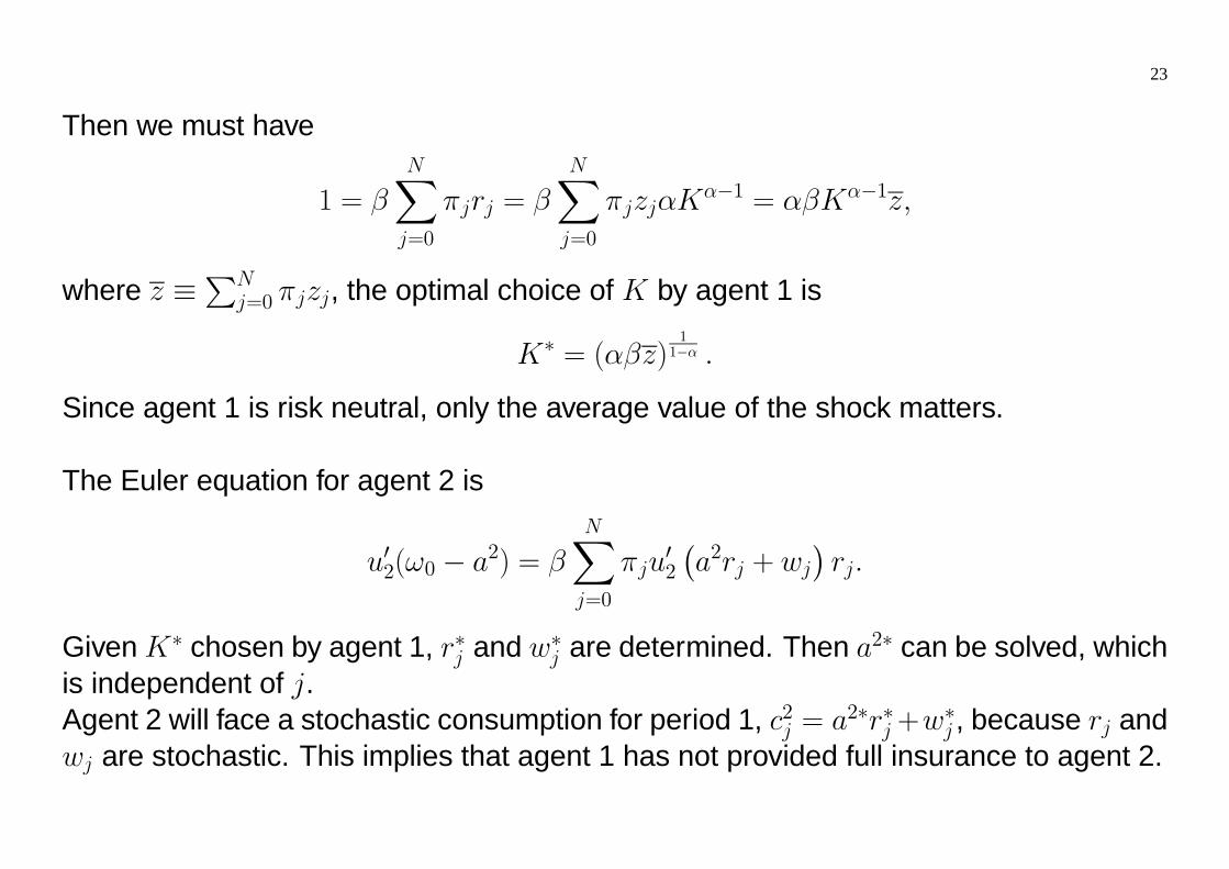
Then we must have

1 = βNXj=0

πjrj = βNXj=0

πjzjαKα−1 = αβKα−1z,

where z ≡PN

j=0 πjzj, the optimal choice of K by agent 1 is

K∗ = (αβz)11−α .

Since agent 1 is risk neutral, only the average value of the shock matters.

The Euler equation for agent 2 is

u02(ω0 − a2) = βNXj=0

πju02

¡a2rj + wj

¢rj.

Given K∗ chosen by agent 1, r∗j and w∗j are determined. Then a2∗ can be solved, whichis independent of j.Agent 2 will face a stochastic consumption for period 1, c2j = a2∗r∗j +w

∗j , because rj and

wj are stochastic. This implies that agent 1 has not provided full insurance to agent 2.

24

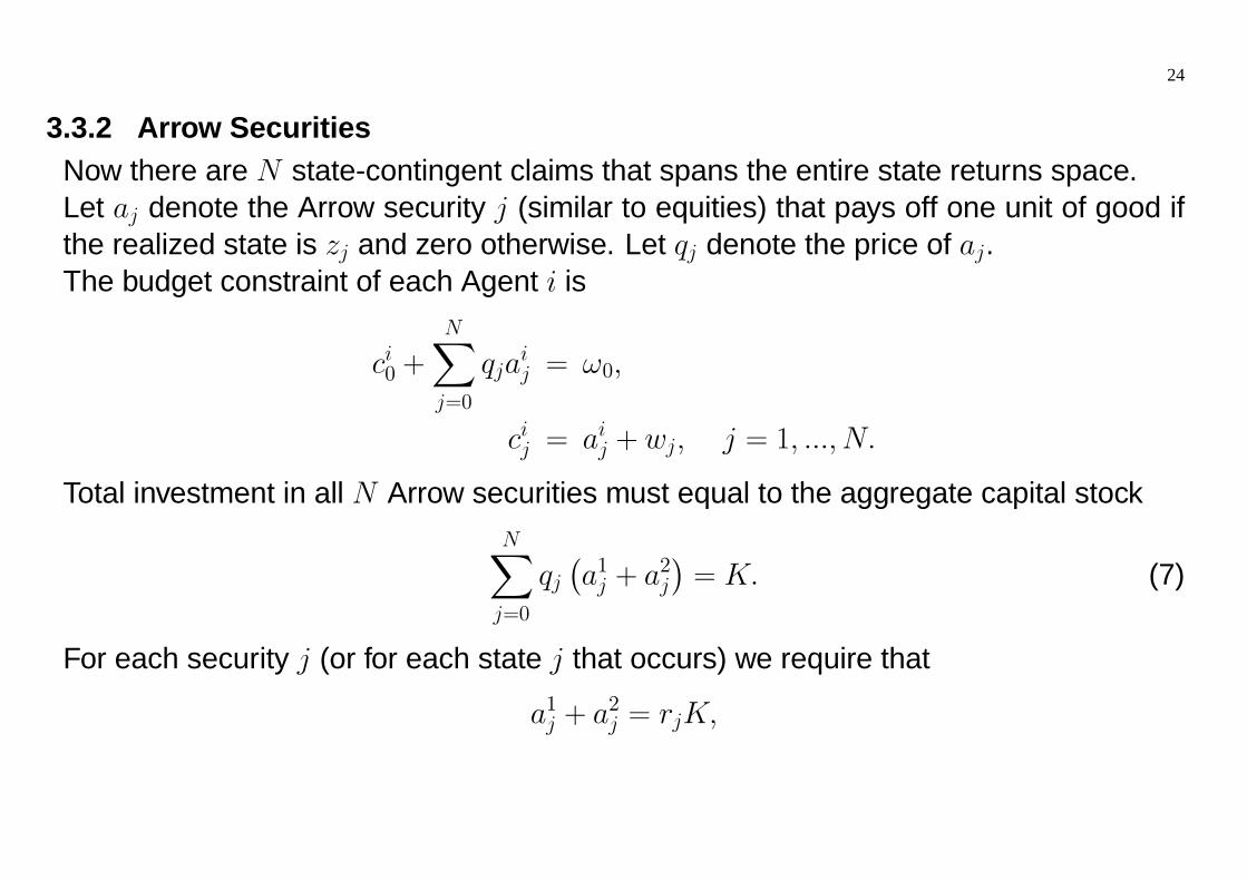
3.3.2 Arrow SecuritiesNow there are N state-contingent claims that spans the entire state returns space.Let aj denote the Arrow security j (similar to equities) that pays off one unit of good ifthe realized state is zj and zero otherwise. Let qj denote the price of aj.The budget constraint of each Agent i is

ci0 +NXj=0

qjaij = ω0,

cij = aij + wj, j = 1, ..., N.

Total investment in all N Arrow securities must equal to the aggregate capital stockNXj=0

qj¡a1j + a2j

¢= K. (7)

For each security j (or for each state j that occurs) we require that

a1j + a2j = rjK,

25

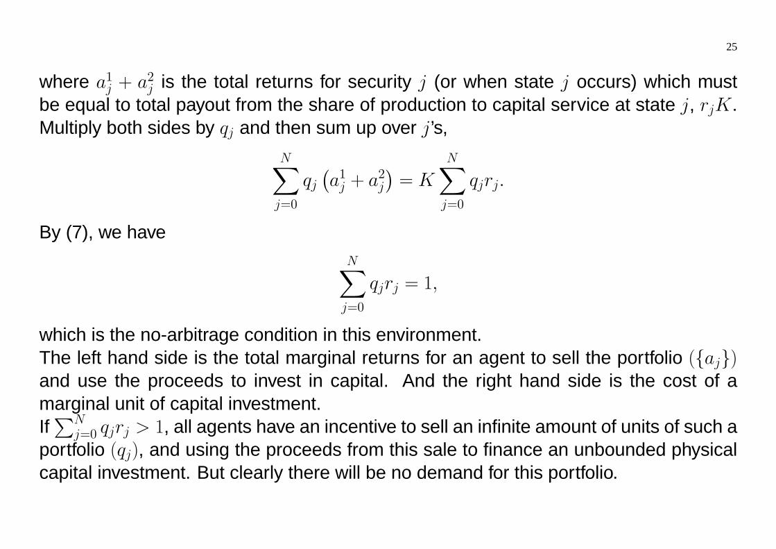
where a1j + a2j is the total returns for security j (or when state j occurs) which mustbe equal to total payout from the share of production to capital service at state j, rjK.Multiply both sides by qj and then sum up over j’s,

NXj=0

qj¡a1j + a2j

¢= K

NXj=0

qjrj.

By (7), we haveNXj=0

qjrj = 1,

which is the no-arbitrage condition in this environment.The left hand side is the total marginal returns for an agent to sell the portfolio ({aj})and use the proceeds to invest in capital. And the right hand side is the cost of amarginal unit of capital investment.IfPN

j=0 qjrj > 1, all agents have an incentive to sell an infinite amount of units of such aportfolio (qj), and using the proceeds from this sale to finance an unbounded physicalcapital investment. But clearly there will be no demand for this portfolio.

26

Using the FOCs of agent 1’s problem, we have

qj = βπj,

and total capital chosen remains to be the same as before

K = (αβz)11−α .

Agent 2’s problem yields the Euler equation

u02(c20)qj = βπju

02

¡c2j¢, for all j.

Using the result qj = βπj, we have

u02(c20) = u02

¡c2j¢, for all j.

which implies agent 2 is fully insured from agent 1, and agent 1 bears all the risk. Notethat in general the asset price depends on MRS of the agent, reflecting how much theagent is willing to purchase insurance. But the risk-neutral agent is willing to bear allthe risk so that the risk-averse agent is able to diversify all the risk re-arranging hisportfolio (purchase more a2j when state j yields a low productivity).