1

Practical Statistics for Physicists

Stockholm Lectures

Sept 2008

Louis Lyons

Imperial College and Oxford

CDF experiment at FNAL

CMS expt at LHC

l.lyons@physics.ox.ac.uk

2

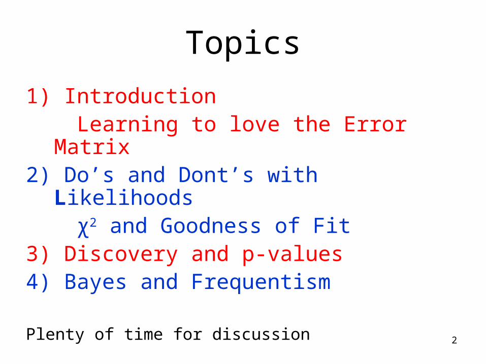
Topics

1) Introduction Learning to love the Error Matrix2) Do’s and Dont’s with Likelihoods χ2 and Goodness of Fit3) Discovery and p-values4) Bayes and Frequentism

Plenty of time for discussion

3

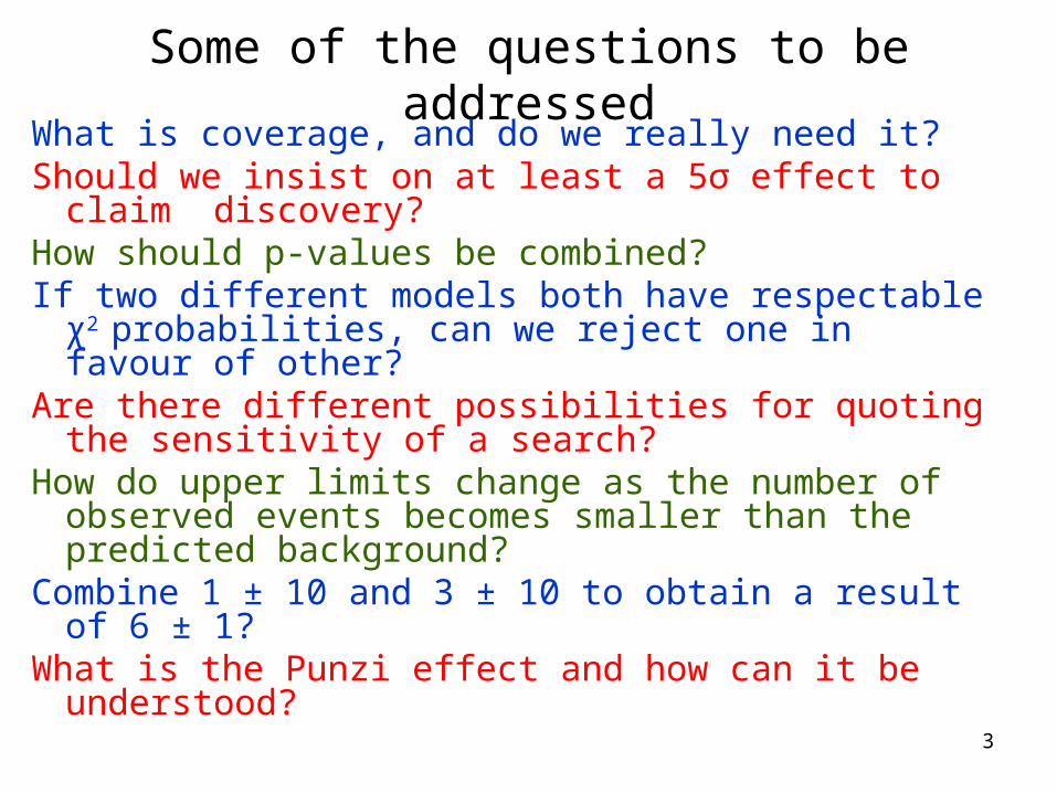
Some of the questions to be addressedWhat is coverage, and do we really need it? Should we insist on at least a 5σ effect to claim

discovery?How should p-values be combined? If two different models both have respectable χ2

probabilities, can we reject one in favour of other?Are there different possibilities for quoting the

sensitivity of a search?How do upper limits change as the number of

observed events becomes smaller than the predicted background?

Combine 1 ± 10 and 3 ± 10 to obtain a result of 6 ± 1? What is the Punzi effect and how can it be

understood?

4

Books

Statistics for Nuclear and Particle Physicists Cambridge University Press, 1986

Available from CUP

Errata in these lectures

5

Other Books

CDF Statistics Committee

BaBar Statistics Working Group

6

7

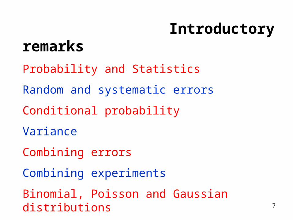
Introductory remarks

Probability and Statistics

Random and systematic errors

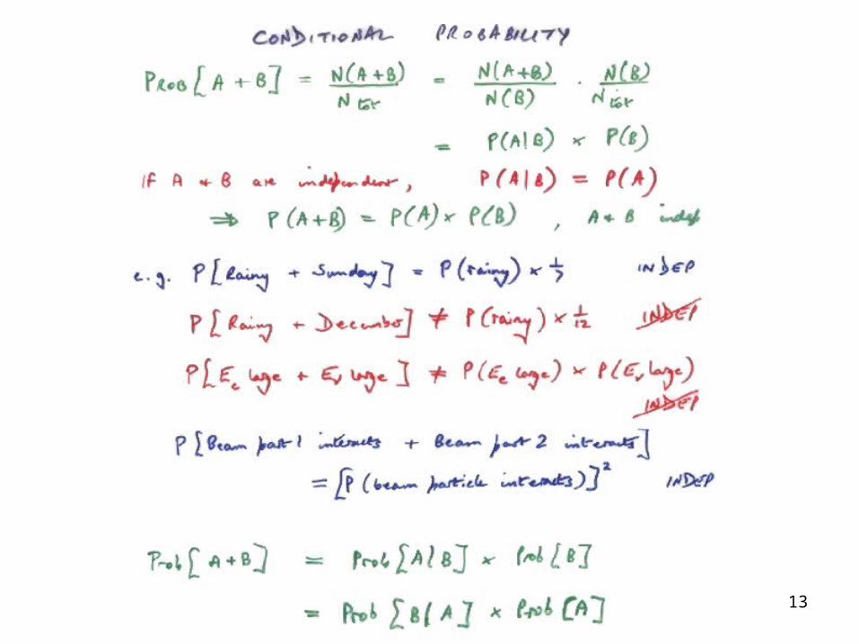
Conditional probability

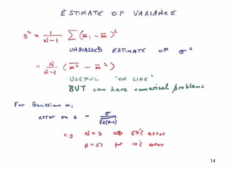
Variance

Combining errors

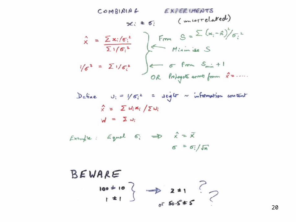
Combining experiments

Binomial, Poisson and Gaussian distributions

8

9

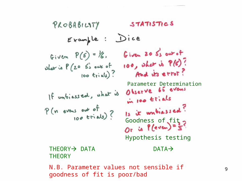
Parameter Determination

Goodness of fit

Hypothesis testing

THEORY DATA DATA THEORY

N.B. Parameter values not sensible if goodness of fit is poor/bad

10

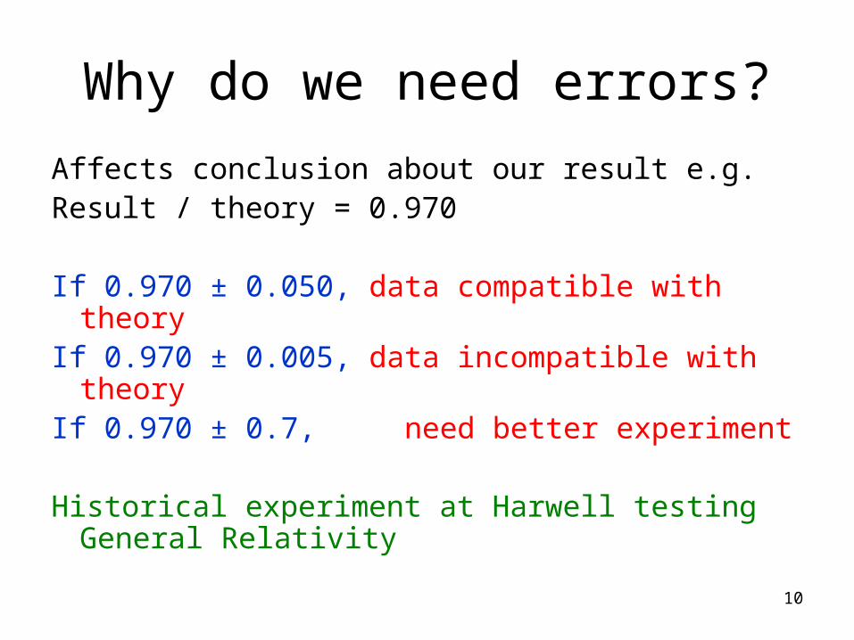
Why do we need errors?

Affects conclusion about our result e.g.Result / theory = 0.970

If 0.970 ± 0.050, data compatible with theory If 0.970 ± 0.005, data incompatible with theoryIf 0.970 ± 0.7, need better experiment

Historical experiment at Harwell testing General Relativity

11

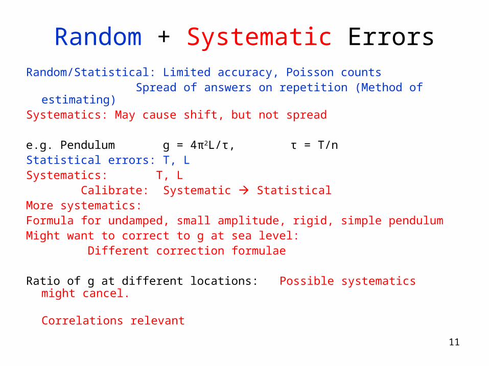
Random + Systematic ErrorsRandom/Statistical: Limited accuracy, Poisson counts Spread of answers on repetition (Method of estimating)Systematics: May cause shift, but not spread

e.g. Pendulum g = 4π2L/τ, τ = T/nStatistical errors: T, LSystematics: T, L Calibrate: Systematic StatisticalMore systematics:Formula for undamped, small amplitude, rigid, simple pendulumMight want to correct to g at sea level: Different correction formulae

Ratio of g at different locations: Possible systematics might cancel. Correlations relevant

12

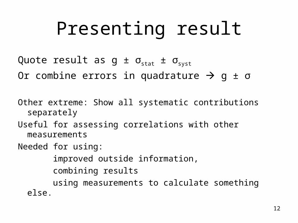
Presenting result

Quote result as g ± σstat ± σsyst

Or combine errors in quadrature g ± σ

Other extreme: Show all systematic contributions separately

Useful for assessing correlations with other measurements

Needed for using:

improved outside information,

combining results

using measurements to calculate something else.

13

14

15

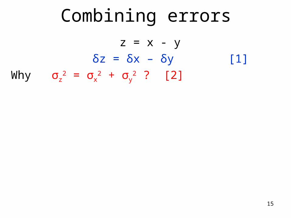
Combining errors z = x - y

δz = δx – δy [1]

Why σz2 = σx

2 + σy2 ? [2]

16

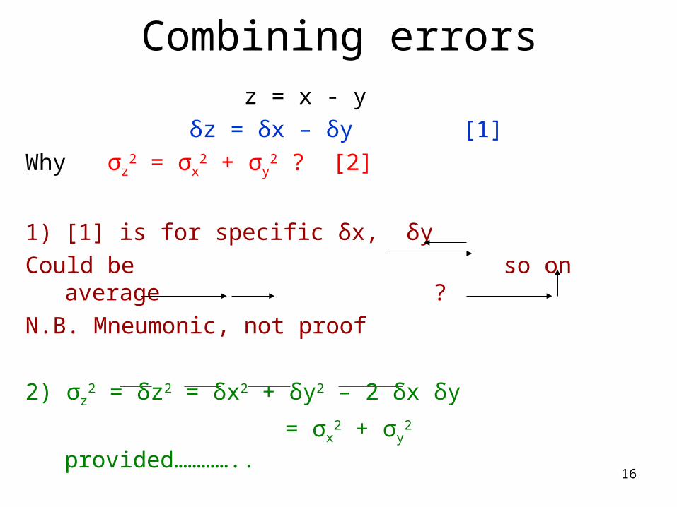
Combining errors z = x - y

δz = δx – δy [1]

Why σz2 = σx

2 + σy2 ? [2]

1) [1] is for specific δx, δy

Could be so on average ?

N.B. Mneumonic, not proof

2) σz2 = δz2 = δx2 + δy2 – 2 δx δy

= σx2 + σy

2 provided…………..

17

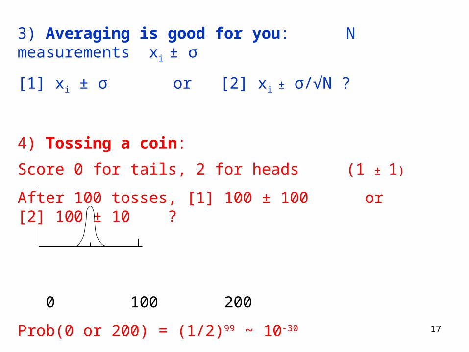
3) Averaging is good for you: N measurements xi ± σ

[1] xi ± σ or [2] xi ± σ/√N ?

4) Tossing a coin:

Score 0 for tails, 2 for heads (1 ± 1)

After 100 tosses, [1] 100 ± 100 or [2] 100 ± 10 ?

0 100 200

Prob(0 or 200) = (1/2)99 ~ 10-30

Compare age of Universe ~ 1018 seconds

18

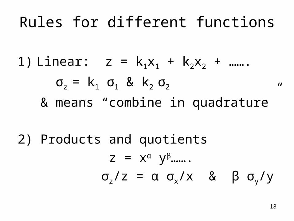
Rules for different functions

1) Linear: z = k1x1 + k2x2 + …….

σz = k1 σ1 & k2 σ2

& means “combine in quadrature”

2) Products and quotients

z = xα yβ…….

σz/z = α σx/x & β σy/y

19

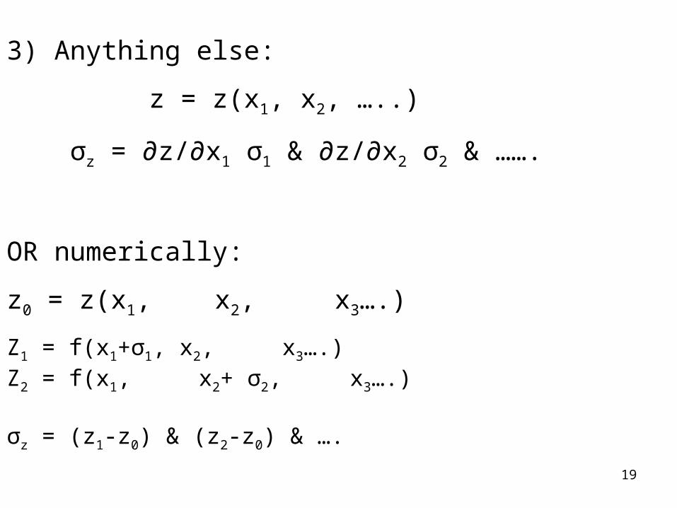
3) Anything else:

z = z(x1, x2, …..)

σz = ∂z/∂x1 σ1 & ∂z/∂x2 σ2 & …….

OR numerically:

z0 = z(x1, x2, x3….)

Z1 = f(x1+σ1, x2, x3….)Z2 = f(x1, x2+ σ2, x3….)

σz = (z1-z0) & (z2-z0) & ….

20

21

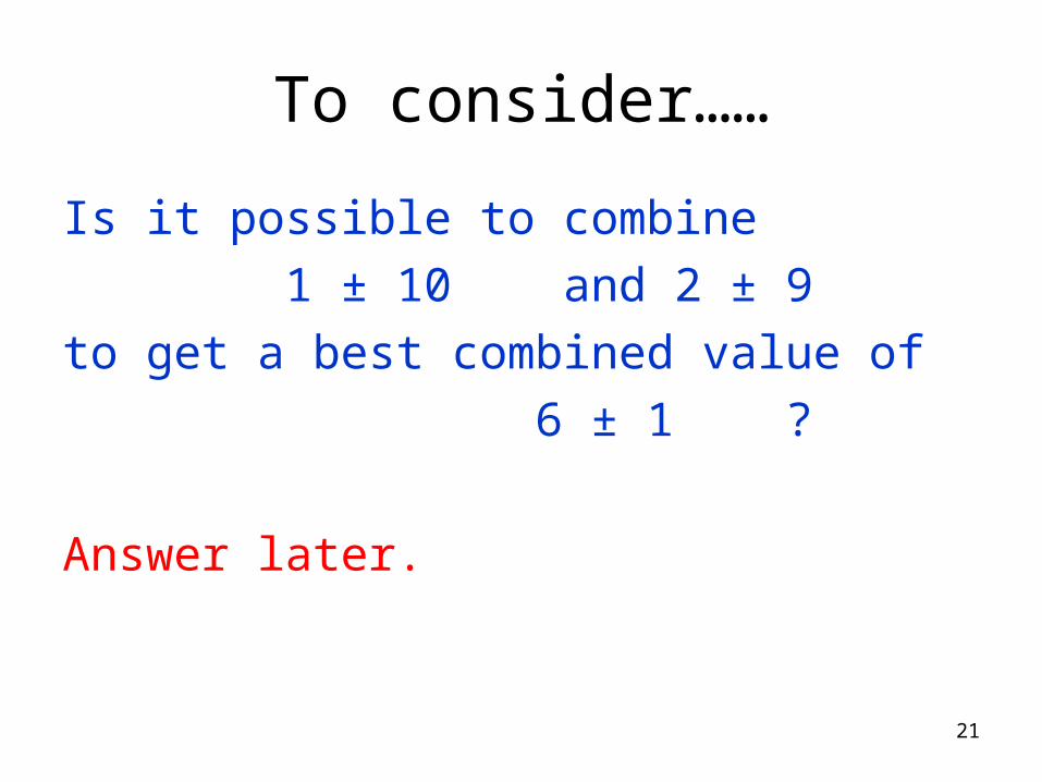
To consider……

Is it possible to combine

1 ± 10 and 2 ± 9

to get a best combined value of

6 ± 1 ?

Answer later.

22

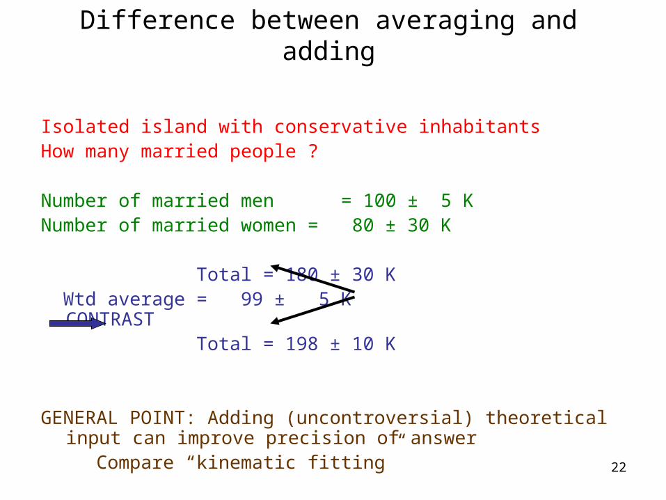
Difference between averaging and adding

Isolated island with conservative inhabitantsHow many married people ?

Number of married men = 100 ± 5 KNumber of married women = 80 ± 30 K

Total = 180 ± 30 K Wtd average = 99 ± 5 K CONTRAST Total = 198 ± 10 K

GENERAL POINT: Adding (uncontroversial) theoretical input can improve precision of answer

Compare “kinematic fitting”

23

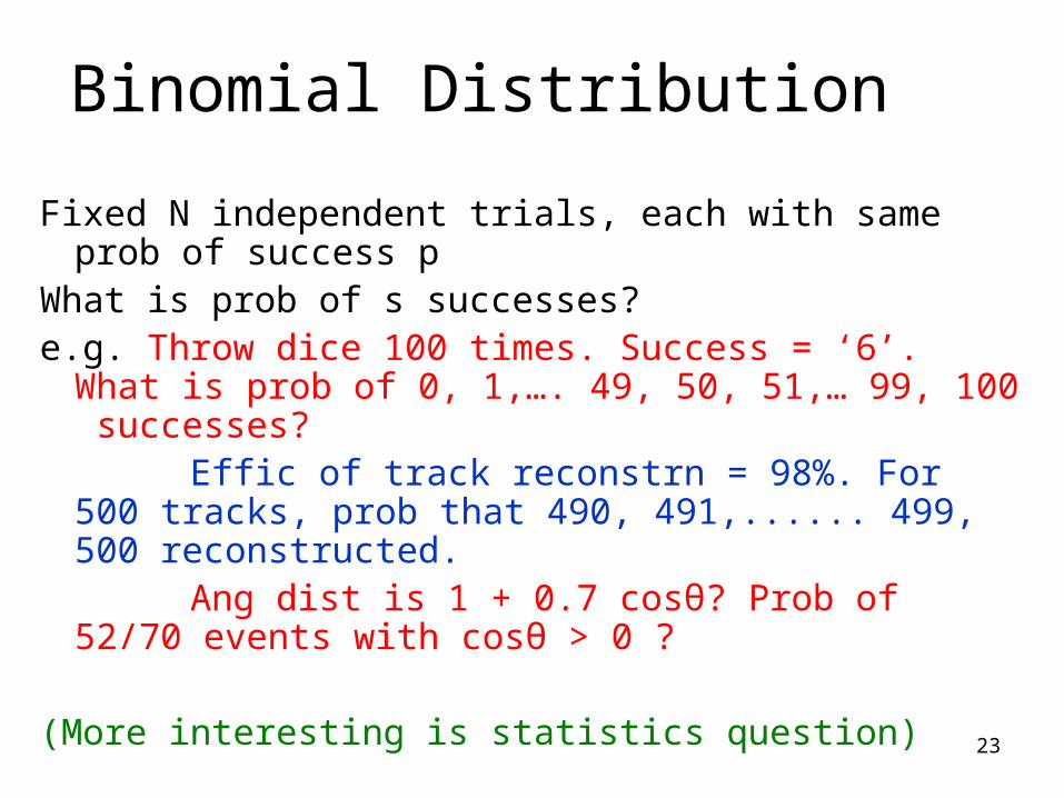
Binomial Distribution

Fixed N independent trials, each with same prob of success p

What is prob of s successes?e.g. Throw dice 100 times. Success = ‘6’. What is

prob of 0, 1,…. 49, 50, 51,… 99, 100 successes? Effic of track reconstrn = 98%. For 500 tracks,

prob that 490, 491,...... 499, 500 reconstructed. Ang dist is 1 + 0.7 cosθ? Prob of 52/70 events

with cosθ > 0 ?

(More interesting is statistics question)

24

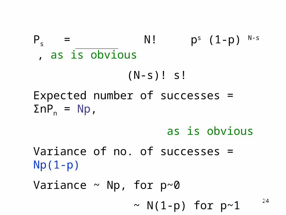
Ps = N! ps (1-p) N-s , as is obvious

(N-s)! s!

Expected number of successes = ΣnPn = Np,

as is obvious

Variance of no. of successes = Np(1-p)

Variance ~ Np, for p~0

~ N(1-p) for p~1

NOT Np in general. NOT n ±√n

25

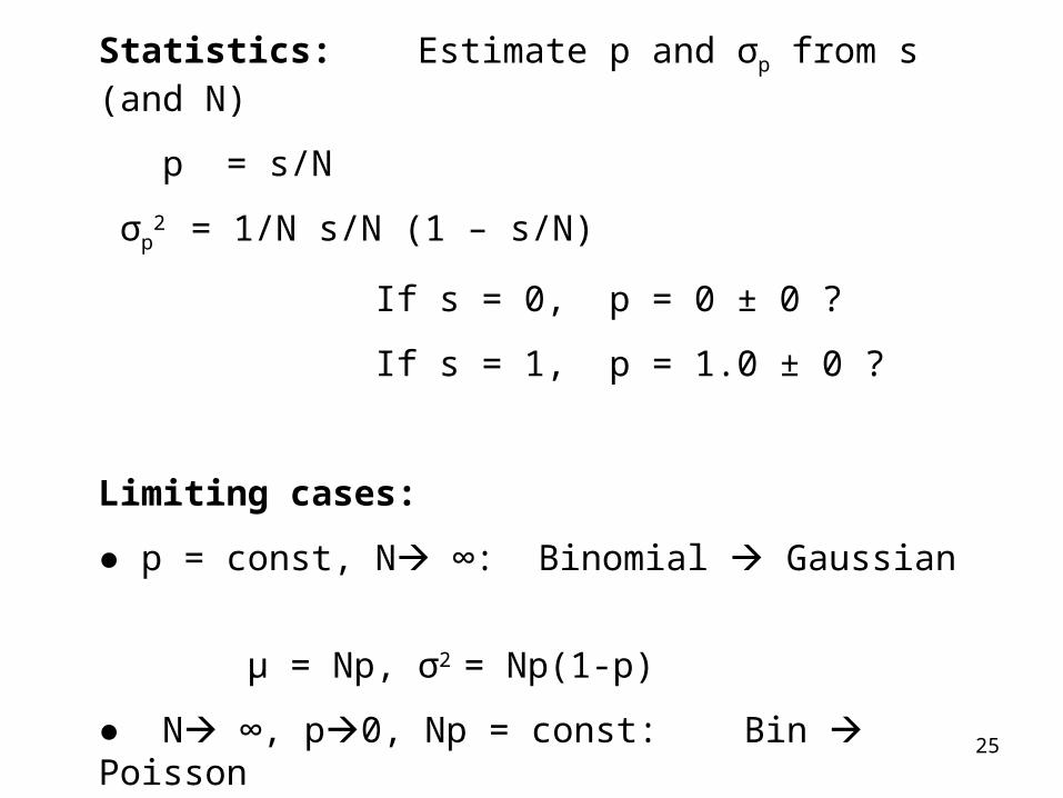
Statistics: Estimate p and σp from s (and N)

p = s/N

σp2

= 1/N s/N (1 – s/N)

If s = 0, p = 0 ± 0 ?

If s = 1, p = 1.0 ± 0 ?

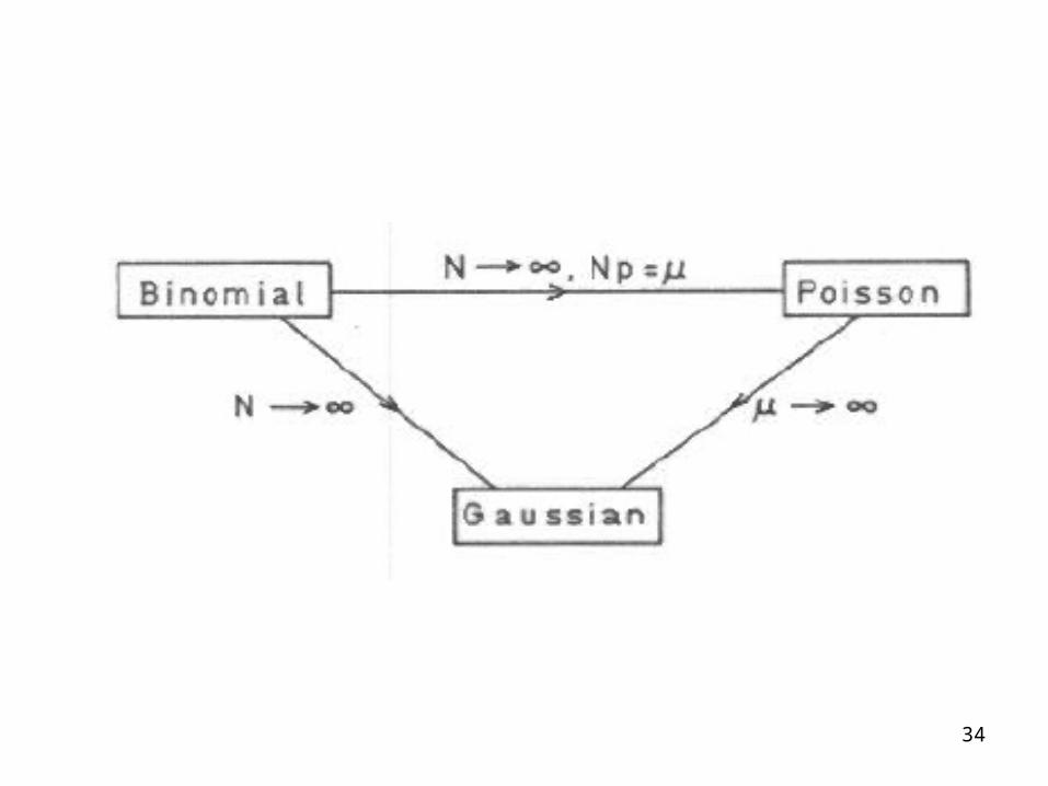
Limiting cases:

● p = const, N ∞: Binomial Gaussian

μ = Np, σ2 = Np(1-p)

● N ∞, p0, Np = const: Bin Poisson

μ = Np, σ2 = Np

{N.B. Gaussian continuous and extends to -∞}

26

27

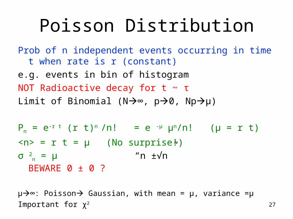
Poisson DistributionProb of n independent events occurring in time t when rate

is r (constant)

e.g. events in bin of histogram

NOT Radioactive decay for t ~ τ

Limit of Binomial (N∞, p0, Npμ)

Pn = e-r t (r t)n /n! = e -μ μn/n! (μ = r t)

<n> = r t = μ (No surprise!)

σ 2n = μ “n ±√n” BEWARE 0 ± 0 ?

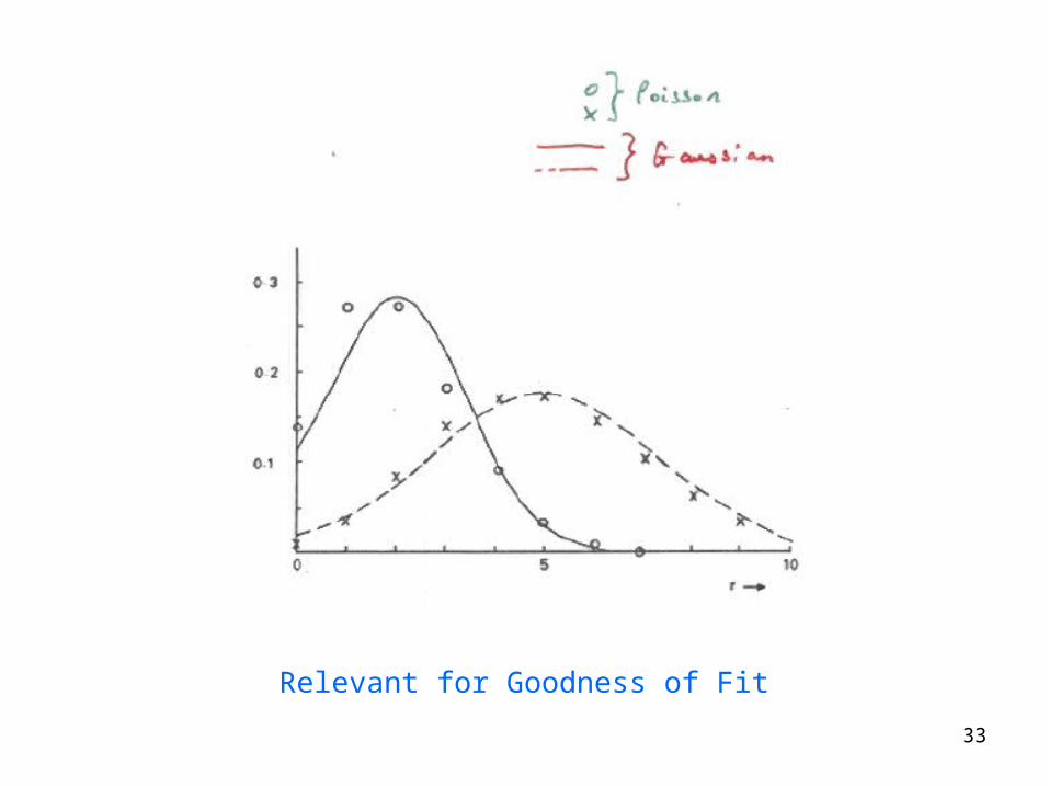
μ∞: Poisson Gaussian, with mean = μ, variance =μ

Important for χ2

28

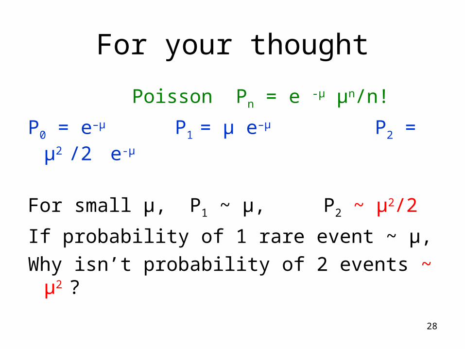
For your thought

Poisson Pn = e -μ μn/n!

P0 = e–μ P1 = μ e–μ P2 = μ2 /2 e-μ

For small μ, P1 ~ μ, P2 ~ μ2/2

If probability of 1 rare event ~ μ,

Why isn’t probability of 2 events ~ μ2 ?

29

30

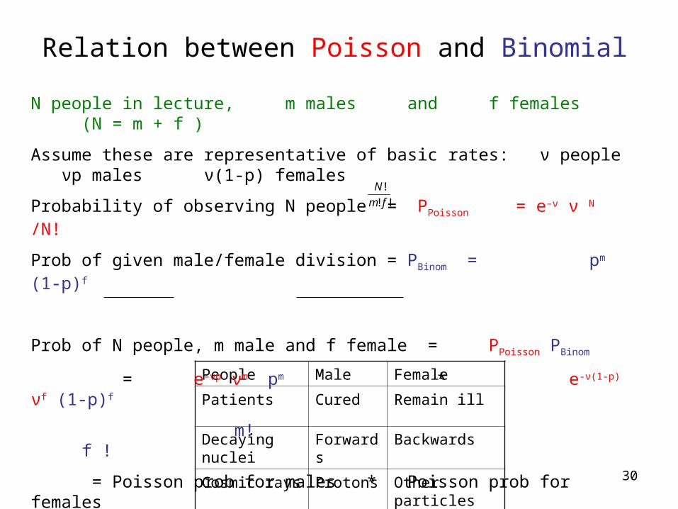
Relation between Poisson and Binomial

!!

!

fm

N

People Male Female

Patients Cured Remain ill

Decaying nuclei

Forwards Backwards

Cosmic rays Protons Other particles

N people in lecture, m males and f females (N = m + f )

Assume these are representative of basic rates: ν people νp males ν(1-p) females

Probability of observing N people = PPoisson = e–ν ν N /N!

Prob of given male/female division = PBinom = pm (1-p)f

Prob of N people, m male and f female = PPoisson PBinom

= e–νp νm pm * e-ν(1-p) νf (1-p)f

m! f !

= Poisson prob for males * Poisson prob for females

31

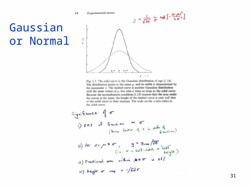
Gaussian or Normal

32

33

Relevant for Goodness of Fit

34

35

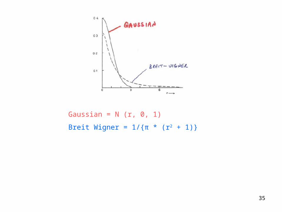
Gaussian = N (r, 0, 1)

Breit Wigner = 1/{π * (r2 + 1)}

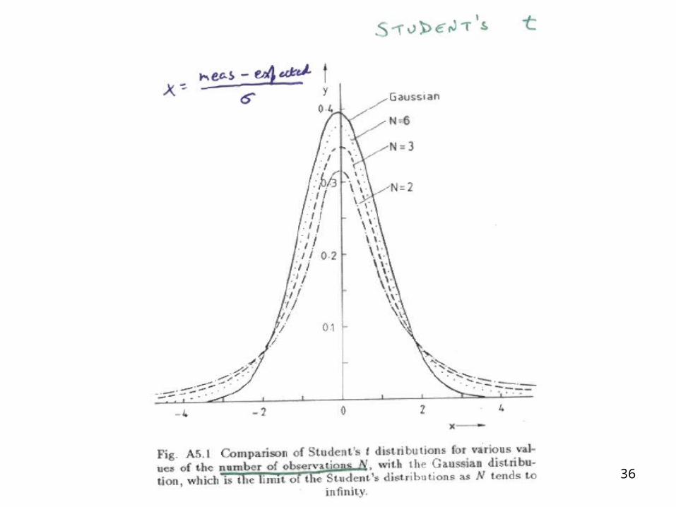
36

37

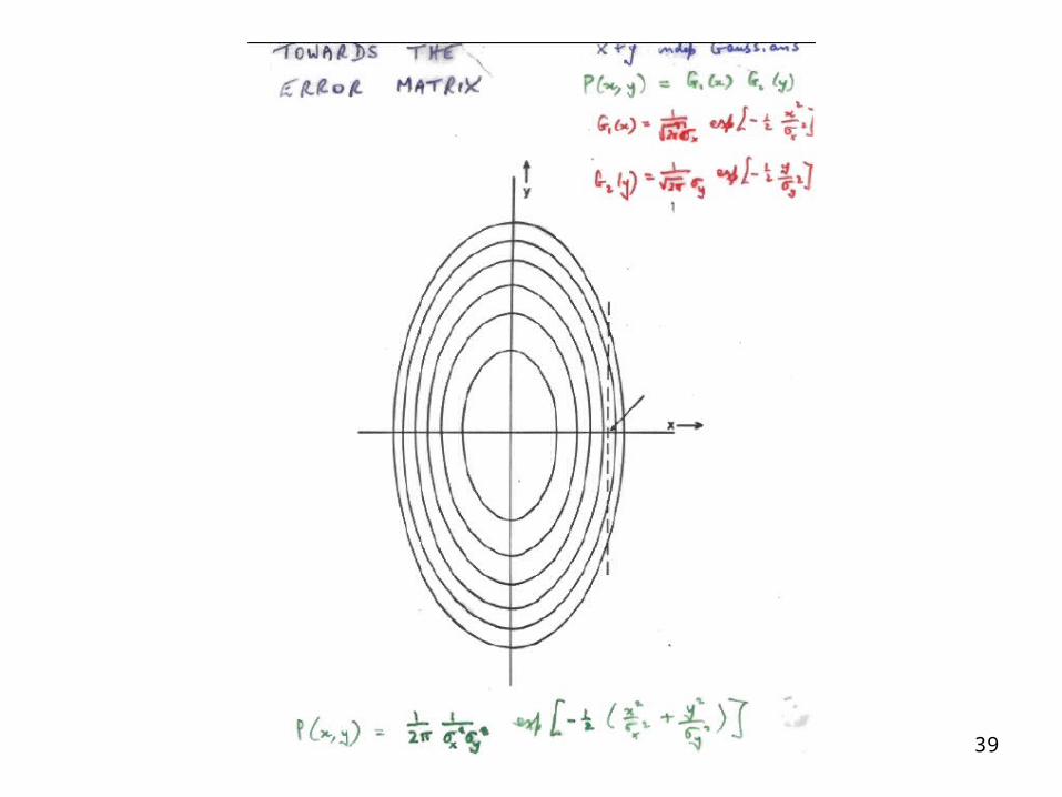
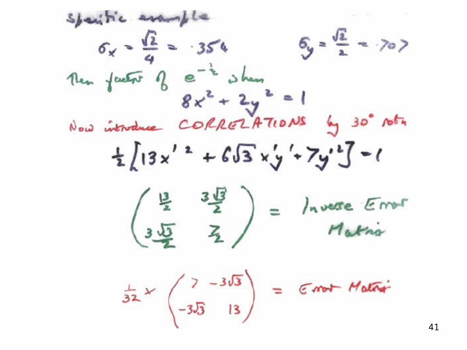
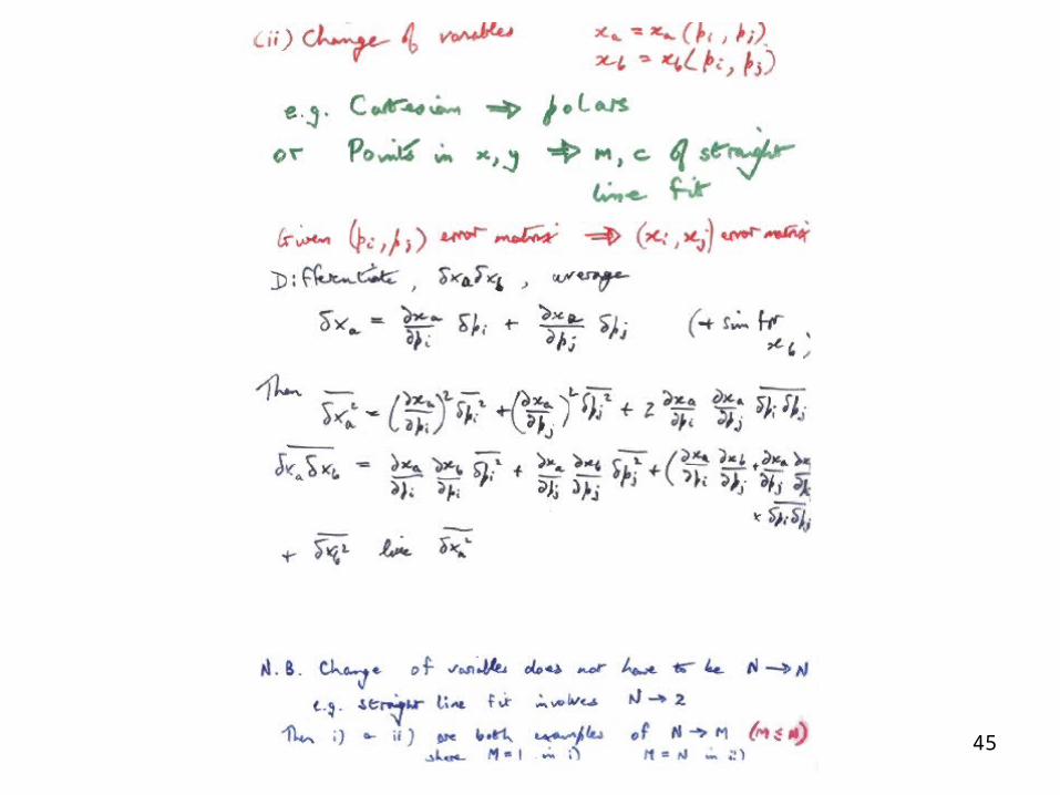
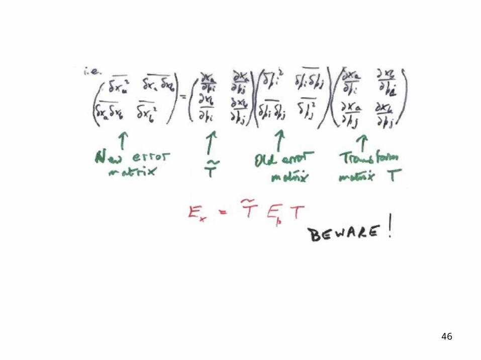
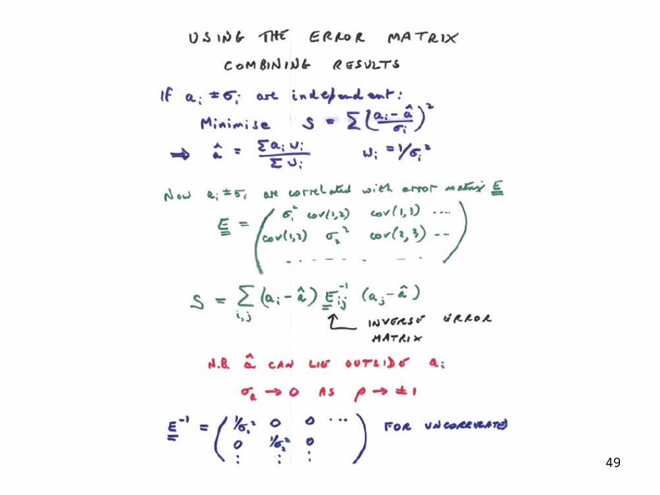
Learning to love the Error Matrix

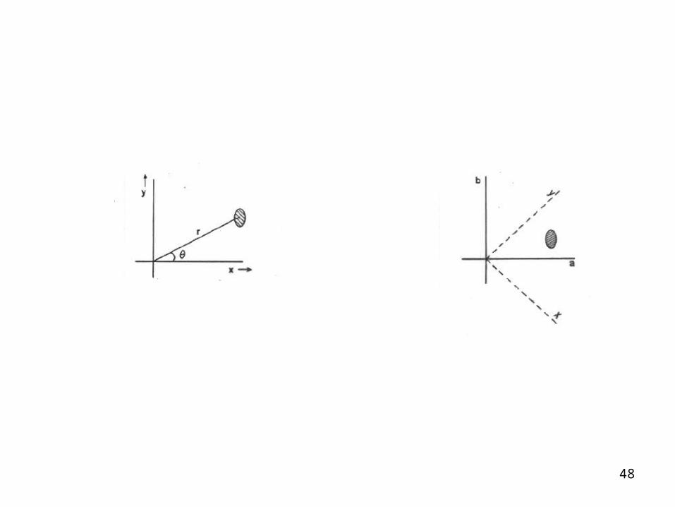
• Introduction via 2-D Gaussian

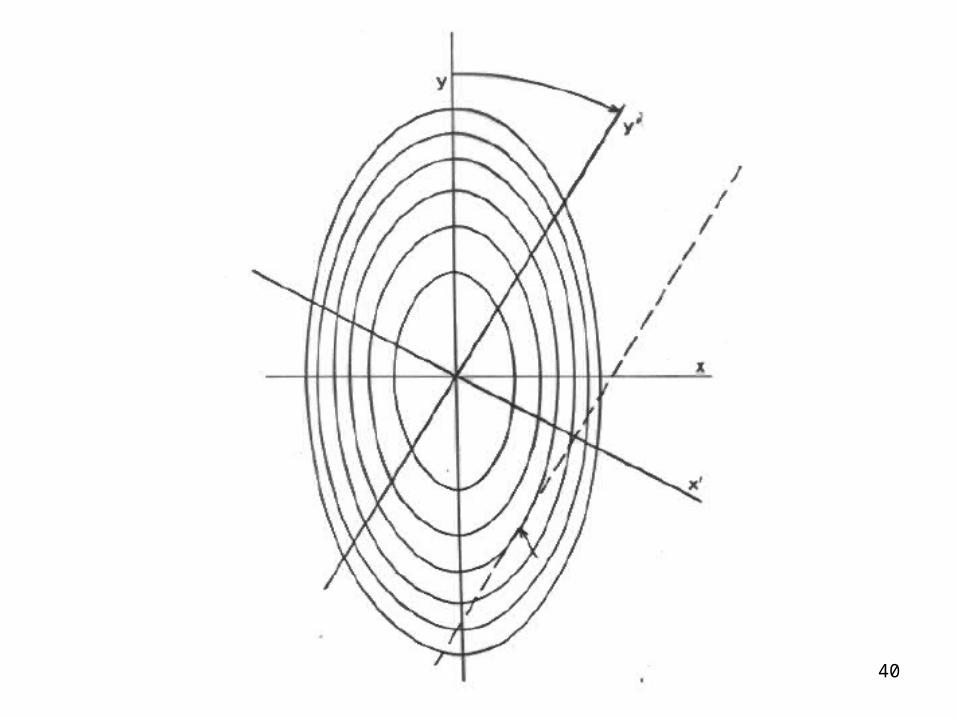
• Understanding covariance

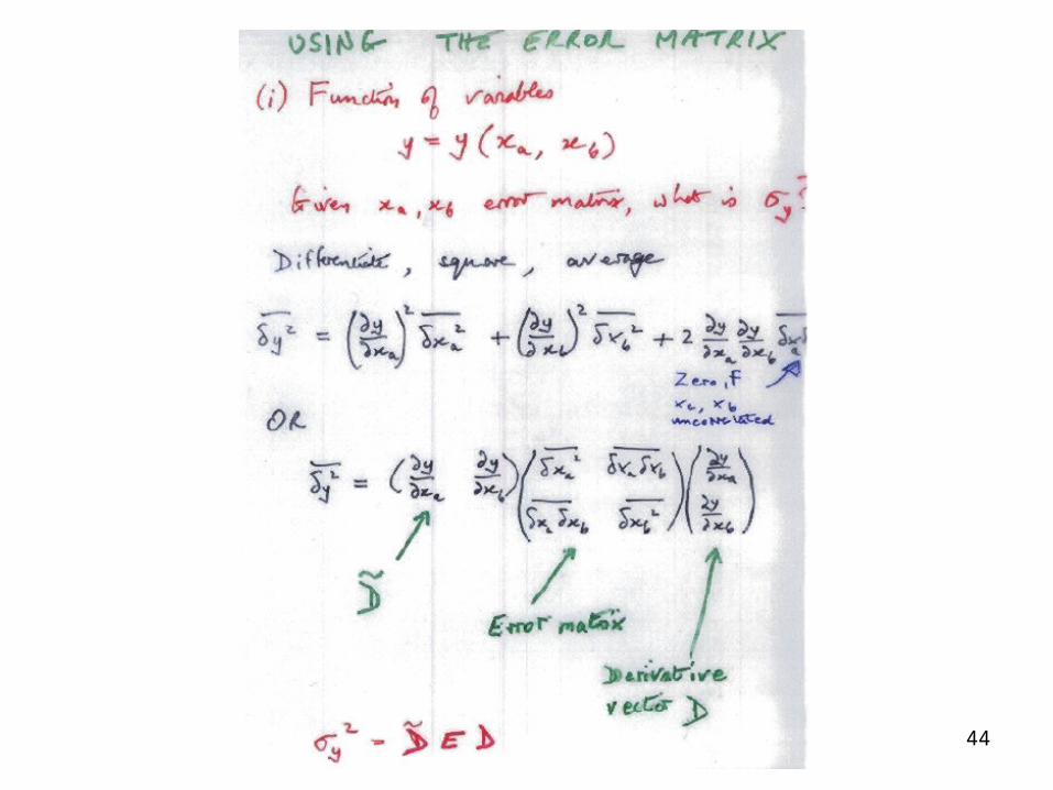
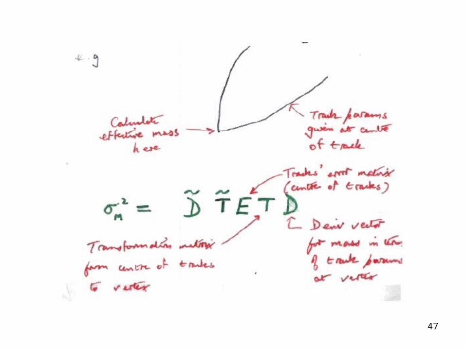
• Using the error matrix

Combining correlated measurements

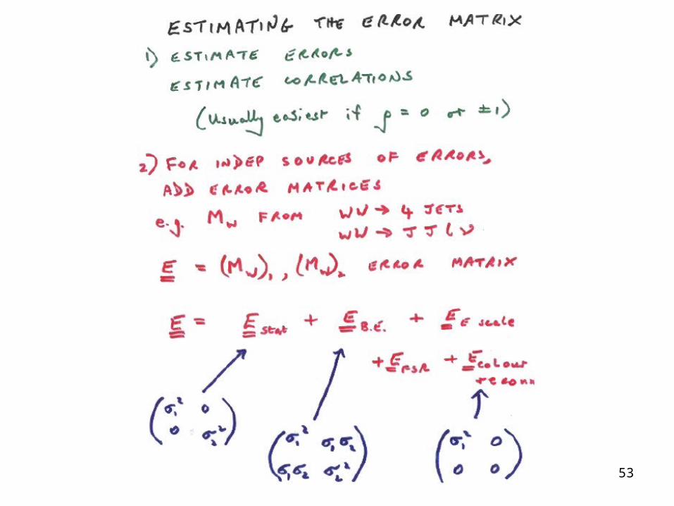
• Estimating the error matrix

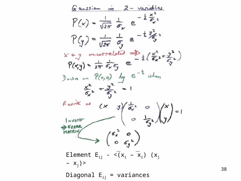
38

Element Eij - <(xi – xi) (xj – xj)>

Diagonal Eij = variances

Off-diagonal Eij = covariances

39

40

41

42

43

44

45

46

47

48

49

50

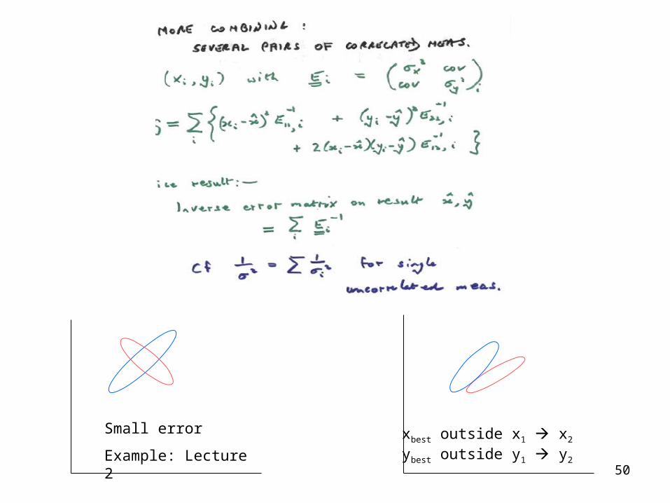
Small error

Example: Lecture 2

xbest outside x1 x2

ybest outside y1 y2

51

a

b

x

y

52

53

54

55

Conclusion

Error matrix formalism makes life easy when correlations are relevant

56

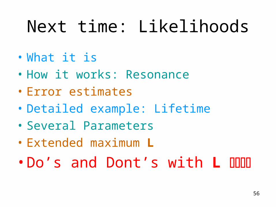
Next time: Likelihoods

• What it is

• How it works: Resonance

• Error estimates

• Detailed example: Lifetime

• Several Parameters

• Extended maximum L

• Do’s and Dont’s with L