1

p-values and Discovery

Louis Lyons

Oxford

l.lyons@physics.ox.ac.uk

SLUO Lecture 4,

February 2007

2

3

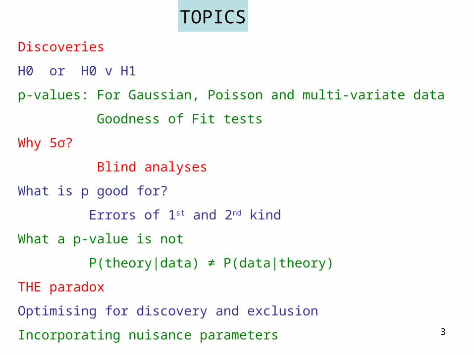
Discoveries

H0 or H0 v H1

p-values: For Gaussian, Poisson and multi-variate data

Goodness of Fit tests

Why 5σ?

Blind analyses

What is p good for?

Errors of 1st and 2nd kind

What a p-value is not

P(theory|data) ≠ P(data|theory)

THE paradox

Optimising for discovery and exclusion

Incorporating nuisance parameters

TOPICS

4

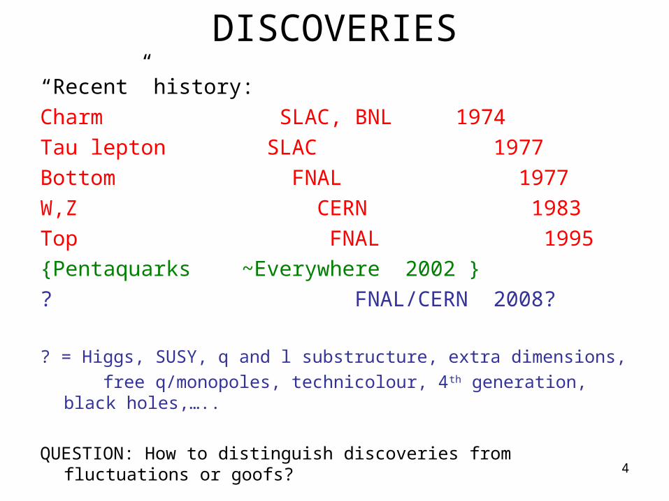
DISCOVERIES

“Recent” history:

Charm SLAC, BNL 1974

Tau lepton SLAC 1977

Bottom FNAL 1977

W,Z CERN 1983

Top FNAL 1995

{Pentaquarks ~Everywhere 2002 }

? FNAL/CERN 2008?

? = Higgs, SUSY, q and l substructure, extra dimensions,

free q/monopoles, technicolour, 4th generation, black holes,…..

QUESTION: How to distinguish discoveries from fluctuations or goofs?

5

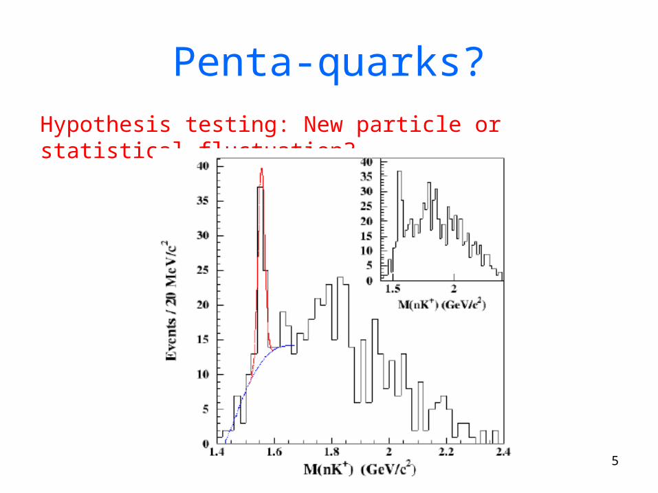
Penta-quarks?

Hypothesis testing: New particle or statistical fluctuation?

6

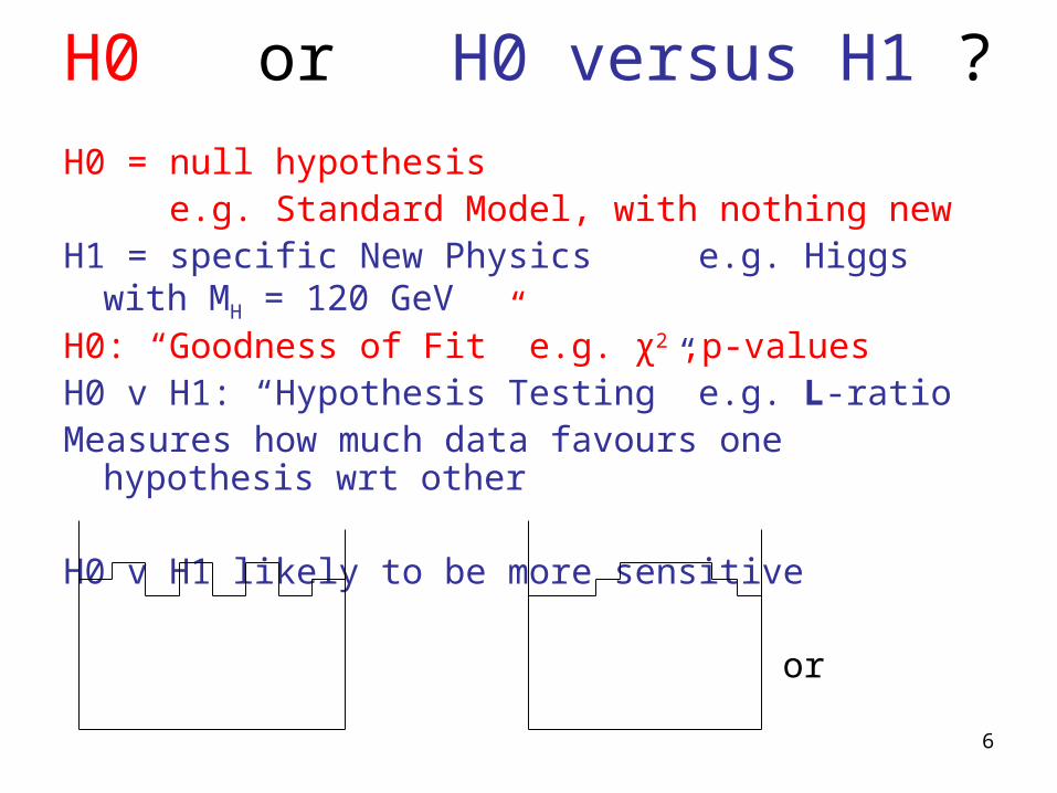
H0 or H0 versus H1 ?

H0 = null hypothesis e.g. Standard Model, with nothing new

H1 = specific New Physics e.g. Higgs with MH = 120 GeV H0: “Goodness of Fit” e.g. χ2 ,p-valuesH0 v H1: “Hypothesis Testing” e.g. L-ratioMeasures how much data favours one hypothesis wrt other

H0 v H1 likely to be more sensitive

or

7

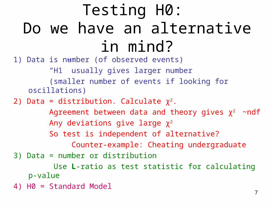
Testing H0: Do we have an alternative in mind?

1) Data is number (of observed events)

“H1” usually gives larger number

(smaller number of events if looking for oscillations)

2) Data = distribution. Calculate χ2.

Agreement between data and theory gives χ2 ~ndf

Any deviations give large χ2

So test is independent of alternative?

Counter-example: Cheating undergraduate

3) Data = number or distribution

Use L-ratio as test statistic for calculating p-value

4) H0 = Standard Model

8

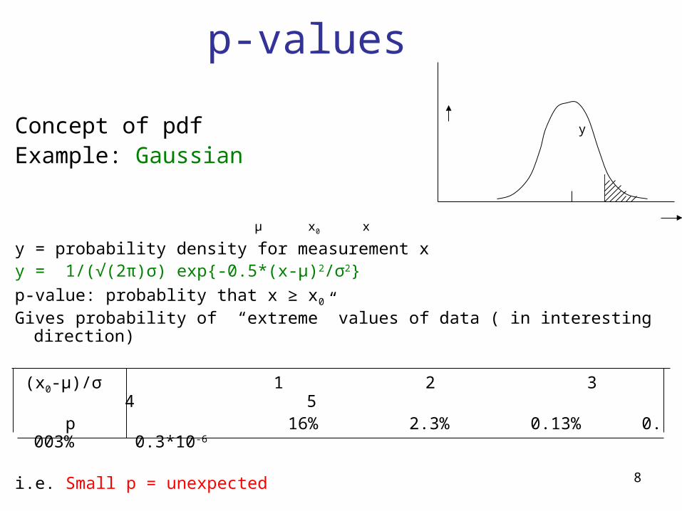
p-values

Concept of pdf y

Example: Gaussian

μ x0 x y = probability density for measurement xy = 1/(√(2π)σ) exp{-0.5*(x-μ)2/σ2}

p-value: probablity that x ≥ x0

Gives probability of “extreme” values of data ( in interesting direction)

(x0-μ)/σ 1 2 3 4 5 p 16% 2.3% 0.13% 0. 003% 0.3*10-6

i.e. Small p = unexpected

9

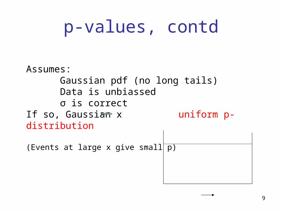
p-values, contd

Assumes: Gaussian pdf (no long tails) Data is unbiassed σ is correctIf so, Gaussian x uniform p-distribution

(Events at large x give small p)

0 p 1

10

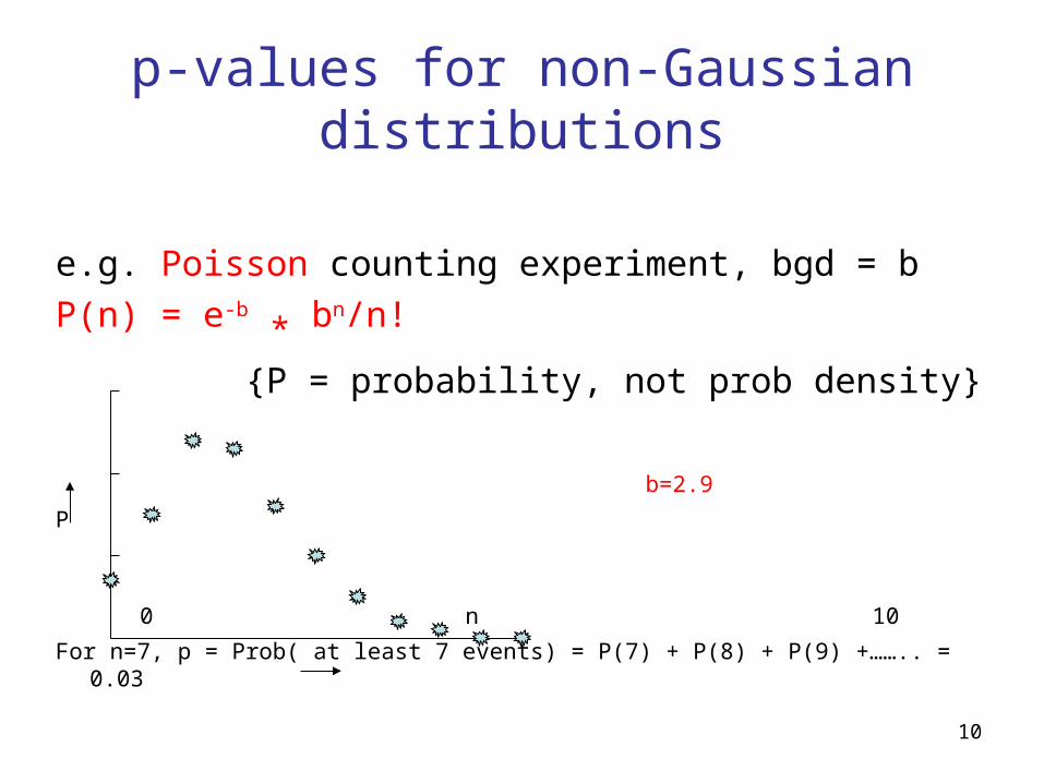
p-values for non-Gaussian distributions

e.g. Poisson counting experiment, bgd = b

P(n) = e-b * bn/n!

{P = probability, not prob density}

b=2.9

P

0 n 10

For n=7, p = Prob( at least 7 events) = P(7) + P(8) + P(9) +…….. = 0.03

11

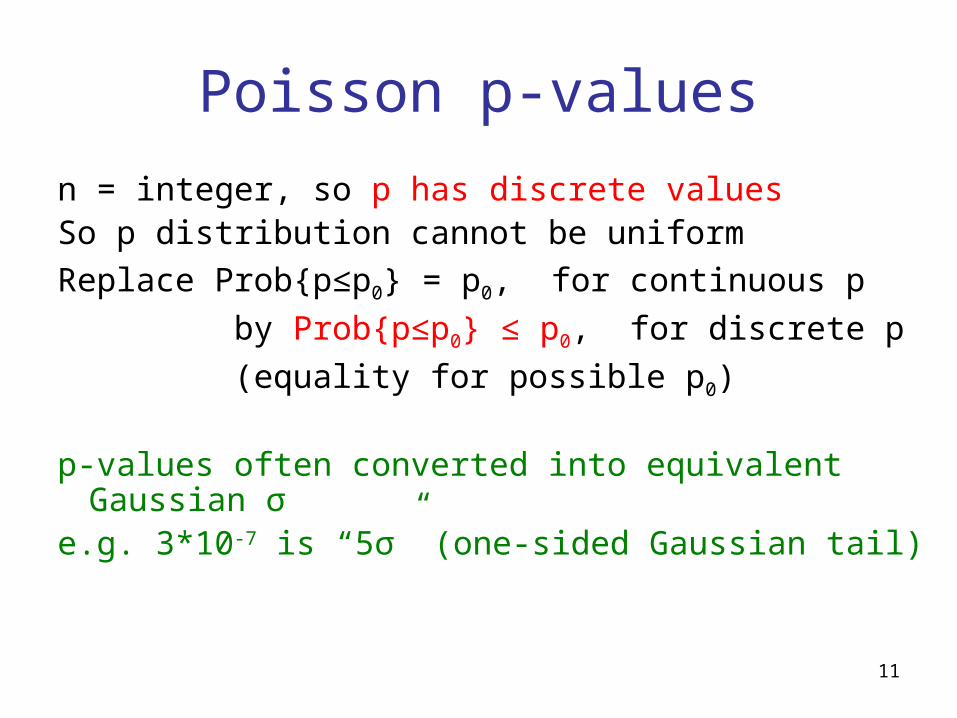
Poisson p-values

n = integer, so p has discrete valuesSo p distribution cannot be uniform

Replace Prob{p≤p0} = p0, for continuous p

by Prob{p≤p0} ≤ p0, for discrete p

(equality for possible p0)

p-values often converted into equivalent Gaussian σ

e.g. 3*10-7 is “5σ” (one-sided Gaussian tail)

12

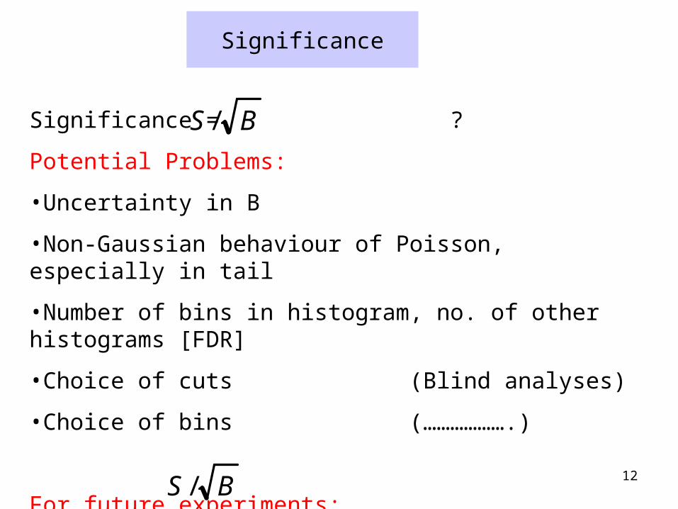
Significance

Significance = ?

Potential Problems:

•Uncertainty in B

•Non-Gaussian behaviour of Poisson, especially in tail

•Number of bins in histogram, no. of other histograms [FDR]

•Choice of cuts (Blind analyses)

•Choice of bins (……………….)

For future experiments:

• Optimising could give S =0.1, B = 10-6

BS /

BS /

13

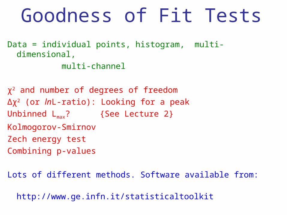
Goodness of Fit TestsData = individual points, histogram, multi-dimensional,

multi-channel

χ2 and number of degrees of freedom

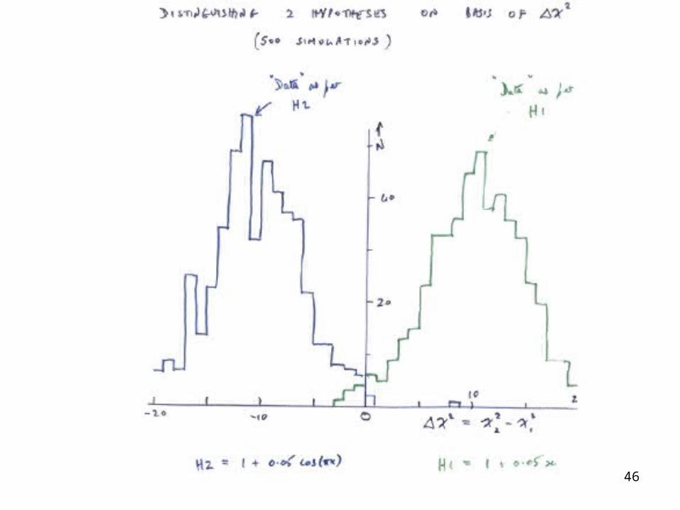
Δχ2 (or lnL-ratio): Looking for a peak

Unbinned Lmax? {See Lecture 2}

Kolmogorov-Smirnov

Zech energy test

Combining p-values

Lots of different methods. Software available from:

http://www.ge.infn.it/statisticaltoolkit

14

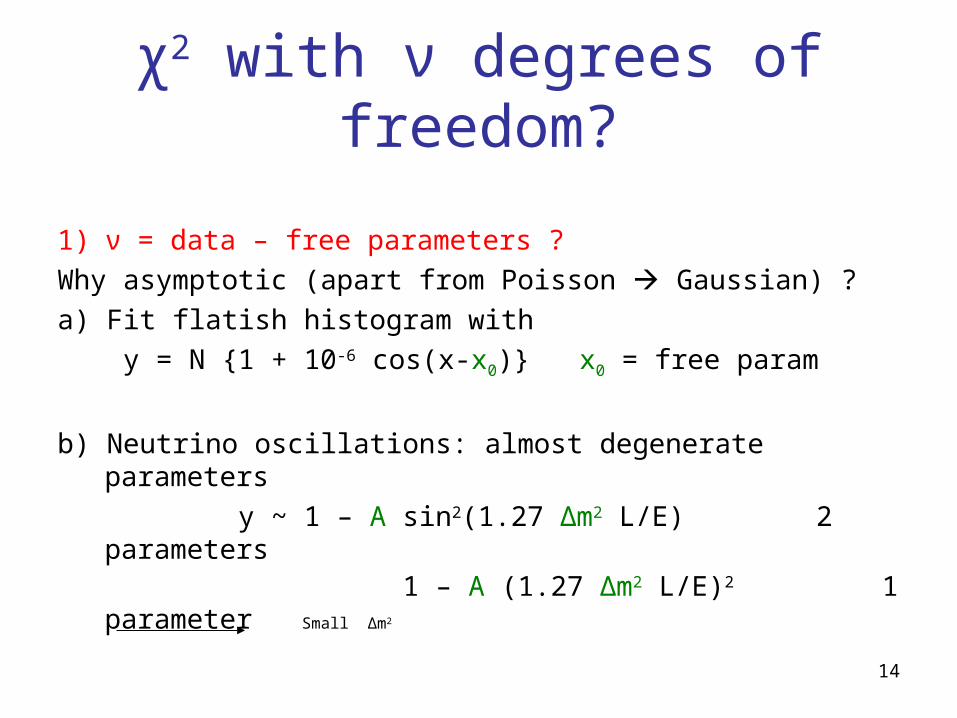
χ2 with ν degrees of freedom?

1) ν = data – free parameters ?

Why asymptotic (apart from Poisson Gaussian) ?

a) Fit flatish histogram with

y = N {1 + 10-6 cos(x-x0)} x0 = free param

b) Neutrino oscillations: almost degenerate parameters

y ~ 1 – A sin2(1.27 Δm2 L/E) 2 parameters 1 – A (1.27 Δm2 L/E)2 1 parameter Small

Δm2

15

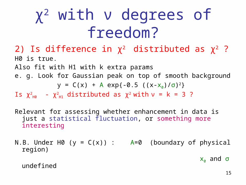
χ2 with ν degrees of freedom?

2) Is difference in χ2 distributed as χ2 ?H0 is true.Also fit with H1 with k extra paramse. g. Look for Gaussian peak on top of smooth background

y = C(x) + A exp{-0.5 ((x-x0)/σ)2}

Is χ2H0

- χ2H1 distributed as χ2 with ν = k = 3 ?

Relevant for assessing whether enhancement in data is just a statistical fluctuation, or something more interesting

N.B. Under H0 (y = C(x)) : A=0 (boundary of physical region)

x0 and σ undefined

16

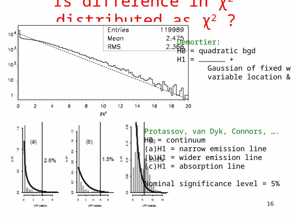
Is difference in χ2 distributed as χ2 ?

Demortier:H0 = quadratic bgdH1 = ……………… + Gaussian of fixed width, variable location & ampl

Protassov, van Dyk, Connors, ….H0 = continuum(a) H1 = narrow emission line(b) H1 = wider emission line(c) H1 = absorption line

Nominal significance level = 5%

17

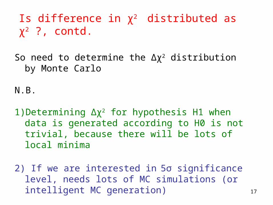
So need to determine the Δχ2 distribution by Monte Carlo

N.B.

1) Determining Δχ2 for hypothesis H1 when data is generated according to H0 is not trivial, because there will be lots of local minima

2) If we are interested in 5σ significance level, needs lots of MC simulations (or intelligent MC generation)

Is difference in χ2 distributed as χ2 ?, contd.

18

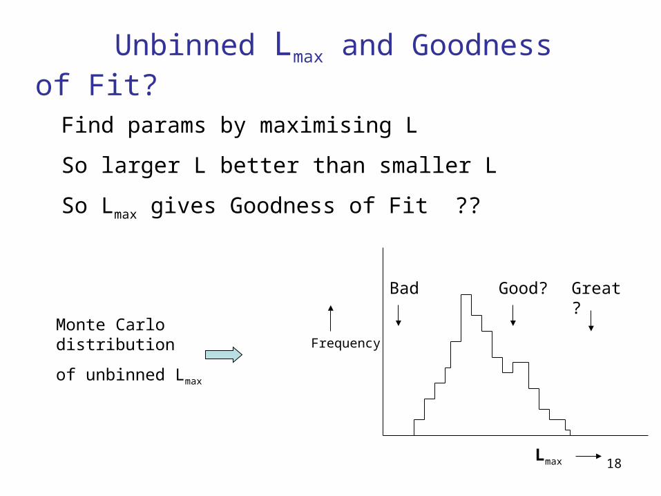
Great?Good?Bad

Lmax

Frequency

Unbinned Lmax and Goodness of Fit?

Find params by maximising L

So larger L better than smaller L

So Lmax gives Goodness of Fit ??

Monte Carlo distribution

of unbinned Lmax

19

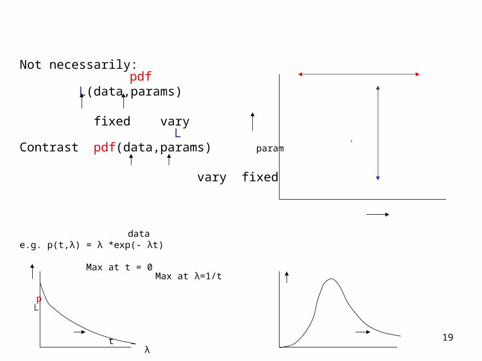
Not necessarily: pdf L(data,params) fixed vary L Contrast pdf(data,params) param

vary fixed

data e.g. p(t,λ) = λ *exp(- λt) Max at t = 0 Max at λ=1/t

p L

t λ

20

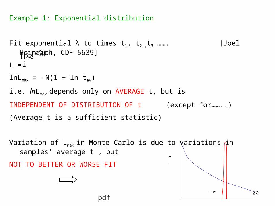
Example 1: Exponential distribution

Fit exponential λ to times t1, t2 ,t3 ……. [Joel Heinrich, CDF 5639]

L =

lnLmax = -N(1 + ln tav)

i.e. lnLmax depends only on AVERAGE t, but is

INDEPENDENT OF DISTRIBUTION OF t (except for……..)

(Average t is a sufficient statistic)

Variation of Lmax in Monte Carlo is due to variations in samples’ average t , but

NOT TO BETTER OR WORSE FIT

pdf

Same average t same Lmax

t

i

e t

21

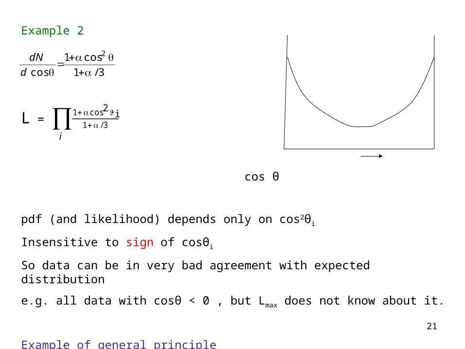
Example 2

L =

cos θ

pdf (and likelihood) depends only on cos2θi

Insensitive to sign of cosθi

So data can be in very bad agreement with expected distribution

e.g. all data with cosθ < 0 , but Lmax does not know about it.

Example of general principle

3/1cos1

cos

2

d

dN

i3/1

cos1 i2

22

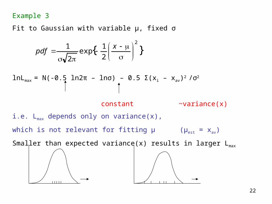
Example 3

Fit to Gaussian with variable μ, fixed σ

lnLmax = N(-0.5 ln2π – lnσ) – 0.5 Σ(xi – xav)2 /σ2

constant ~variance(x)

i.e. Lmax depends only on variance(x),

which is not relevant for fitting μ (μest = xav)

Smaller than expected variance(x) results in larger Lmax

x

x

Worse fit, larger Lmax Better fit, lower Lmax

}{2

2

1exp

2

1

xpdf

23

Lmax and Goodness of Fit?

Conclusion:

L has sensible properties with respect to parameters

NOT with respect to data

Lmax within Monte Carlo peak is NECESSARY

not SUFFICIENT

(‘Necessary’ doesn’t mean that you have to do it!)

24

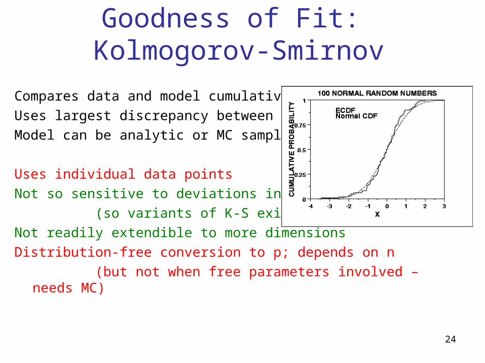
Goodness of Fit: Kolmogorov-Smirnov

Compares data and model cumulative plots

Uses largest discrepancy between dists.

Model can be analytic or MC sample

Uses individual data points

Not so sensitive to deviations in tails

(so variants of K-S exist)

Not readily extendible to more dimensions

Distribution-free conversion to p; depends on n

(but not when free parameters involved – needs MC)

25

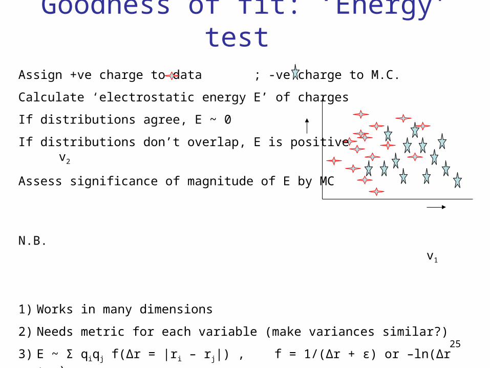
Goodness of fit: ‘Energy’ test

Assign +ve charge to data ; -ve charge to M.C.

Calculate ‘electrostatic energy E’ of charges

If distributions agree, E ~ 0

If distributions don’t overlap, E is positive v2

Assess significance of magnitude of E by MC

N.B. v 1

1) Works in many dimensions

2) Needs metric for each variable (make variances similar?)

3) E ~ Σ qiqj f(Δr = |ri – rj|) , f = 1/(Δr + ε) or –ln(Δr + ε)

Performance insensitive to choice of small ε

See Aslan and Zech’s paper at: http://www.ippp.dur.ac.uk/Workshops/02/statistics/program.shtml

26

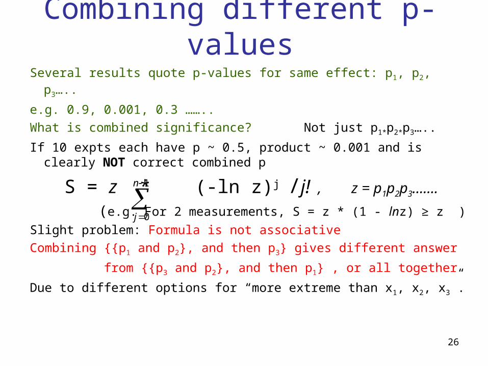
Combining different p-values

Several results quote p-values for same effect: p1, p2, p3…..

e.g. 0.9, 0.001, 0.3 ……..

What is combined significance? Not just p1*p2*p3…..

If 10 expts each have p ~ 0.5, product ~ 0.001 and is clearly NOT correct combined p

S = z * (-ln z)j /j! , z = p1p2p3…….

(e.g. For 2 measurements, S = z * (1 - lnz) ≥ z )

Slight problem: Formula is not associative

Combining {{p1 and p2}, and then p3} gives different answer

from {{p3 and p2}, and then p1} , or all together

Due to different options for “more extreme than x1, x2, x3”.

1

0

n

j

27

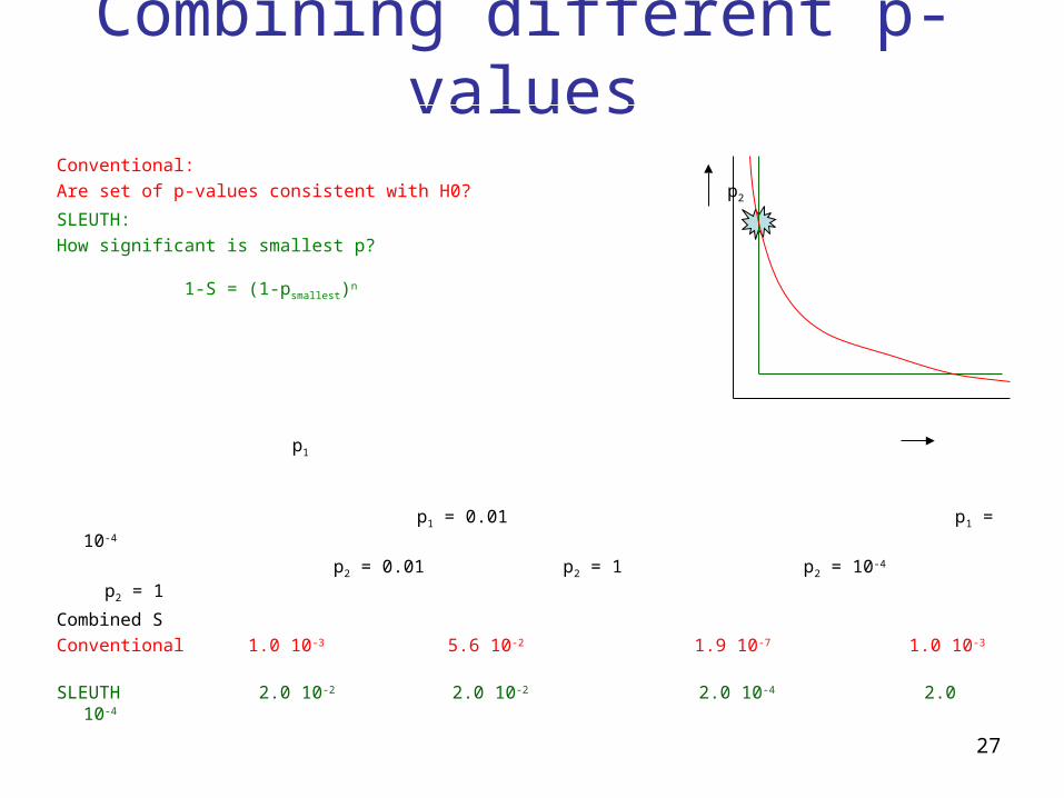
Combining different p-values Conventional:

Are set of p-values consistent with H0? p2

SLEUTH:

How significant is smallest p?

1-S = (1-psmallest)n

p1

p1 = 0.01 p1 = 10-4

p2 = 0.01 p2 = 1 p2 = 10-4 p2 = 1

Combined S

Conventional 1.0 10-3 5.6 10-2 1.9 10-7 1.0 10-3

SLEUTH 2.0 10-2 2.0 10-2 2.0 10-4 2.0 10-4

28

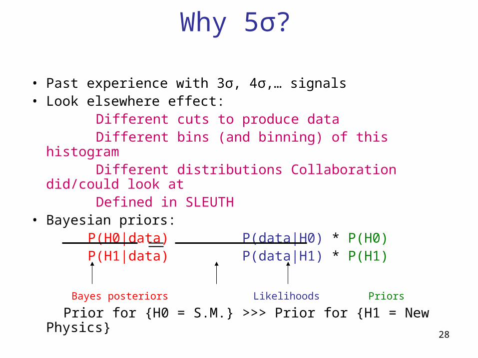
Why 5σ?

• Past experience with 3σ, 4σ,… signals• Look elsewhere effect: Different cuts to produce data Different bins (and binning) of this histogram Different distributions Collaboration did/could look at Defined in SLEUTH• Bayesian priors: P(H0|data) P(data|H0) * P(H0) P(H1|data) P(data|H1) * P(H1)

Bayes posteriors Likelihoods Priors

Prior for {H0 = S.M.} >>> Prior for {H1 = New Physics}

29

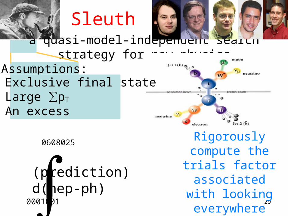
Sleutha quasi-model-independent search strategy for

new physicsAssumptions:

1. Exclusive final state2. Large ∑pT

3. An excess

∫0001001

0608025

(prediction) d(hep-ph)

Rigorously compute the trials factor

associated with looking

everywhere

30

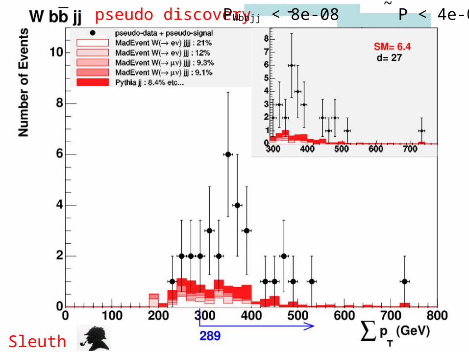
Sleuth

~-pseudo discovery PWbbjj < 8e-08 P < 4e-05

31

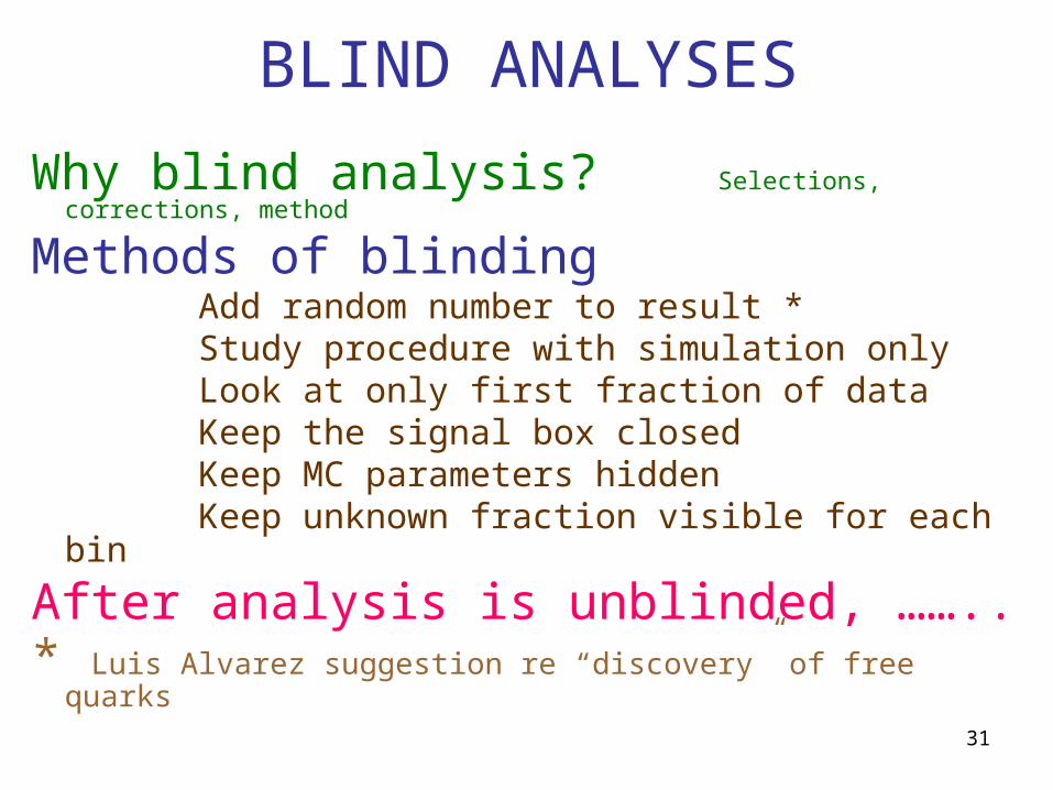
BLIND ANALYSES

Why blind analysis? Selections, corrections, method

Methods of blinding Add random number to result * Study procedure with simulation only Look at only first fraction of data Keep the signal box closed Keep MC parameters hidden Keep unknown fraction visible for each bin

After analysis is unblinded, ……..* Luis Alvarez suggestion re “discovery” of free quarks

32

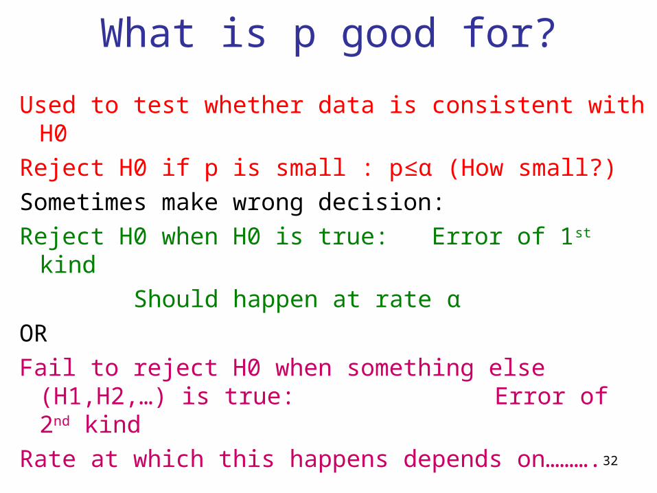
What is p good for?

Used to test whether data is consistent with H0

Reject H0 if p is small : p≤α (How small?)

Sometimes make wrong decision:

Reject H0 when H0 is true: Error of 1st kind

Should happen at rate α

OR

Fail to reject H0 when something else (H1,H2,…) is true: Error of 2nd kind

Rate at which this happens depends on……….

33

Errors of 2nd kind: How often?

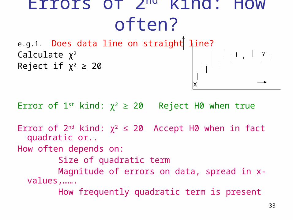
e.g.1. Does data line on straight line?Calculate χ2 y

Reject if χ2 ≥ 20 x

Error of 1st kind: χ2 ≥ 20 Reject H0 when true

Error of 2nd kind: χ2 ≤ 20 Accept H0 when in fact quadratic or..How often depends on: Size of quadratic term Magnitude of errors on data, spread in x-values,……. How frequently quadratic term is present

34

Errors of 2nd kind: How often?

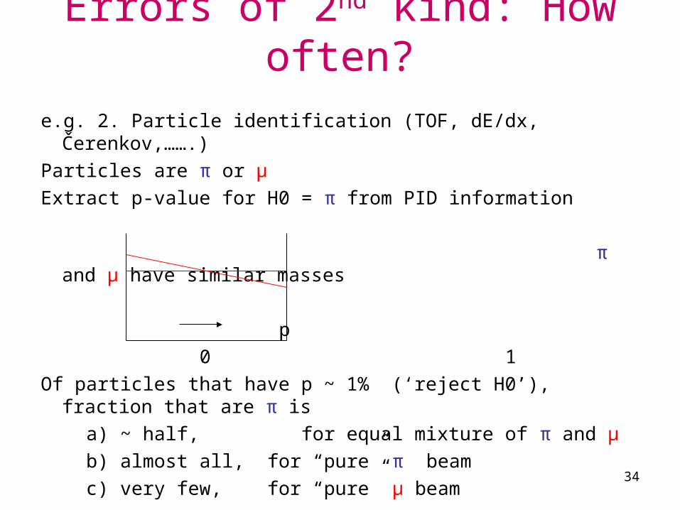
e.g. 2. Particle identification (TOF, dE/dx, Čerenkov,…….)

Particles are π or μ

Extract p-value for H0 = π from PID information

π and μ have similar masses

p

0 1

Of particles that have p ~ 1% (‘reject H0’), fraction that are π is

a) ~ half, for equal mixture of π and μ

b) almost all, for “pure” π beam

c) very few, for “pure” μ beam

35

What is p good for?

Selecting sample of wanted events

e.g. kinematic fit to select t t events

tbW, bjj, Wμν tbW, bjj, Wjj

Convert χ2 from kinematic fit to p-value

Choose cut on χ2 to select t t events

Error of 1st kind: Loss of efficiency for t t events

Error of 2nd kind: Background from other processes

Loose cut (large χ2max

, small pmin): Good efficiency, larger bgd

Tight cut (small χ2max

, larger pmin): Lower efficiency, small bgd

Choose cut to optimise analysis:

More signal events: Reduced statistical error

More background: Larger systematic error

36

p-value is not ……..

Does NOT measure Prob(H0 is true)i.e. It is NOT P(H0|data)It is P(data|H0)N.B. P(H0|data) ≠ P(data|H0) P(theory|data) ≠ P(data|theory)

“Of all results with p ≤ 5%, half will turn out to be wrong”

N.B. Nothing wrong with this statemente.g. 1000 tests of energy conservation~50 should have p ≤ 5%, and so reject H0 =

energy conservationOf these 50 results, all are likely to be “wrong”

37

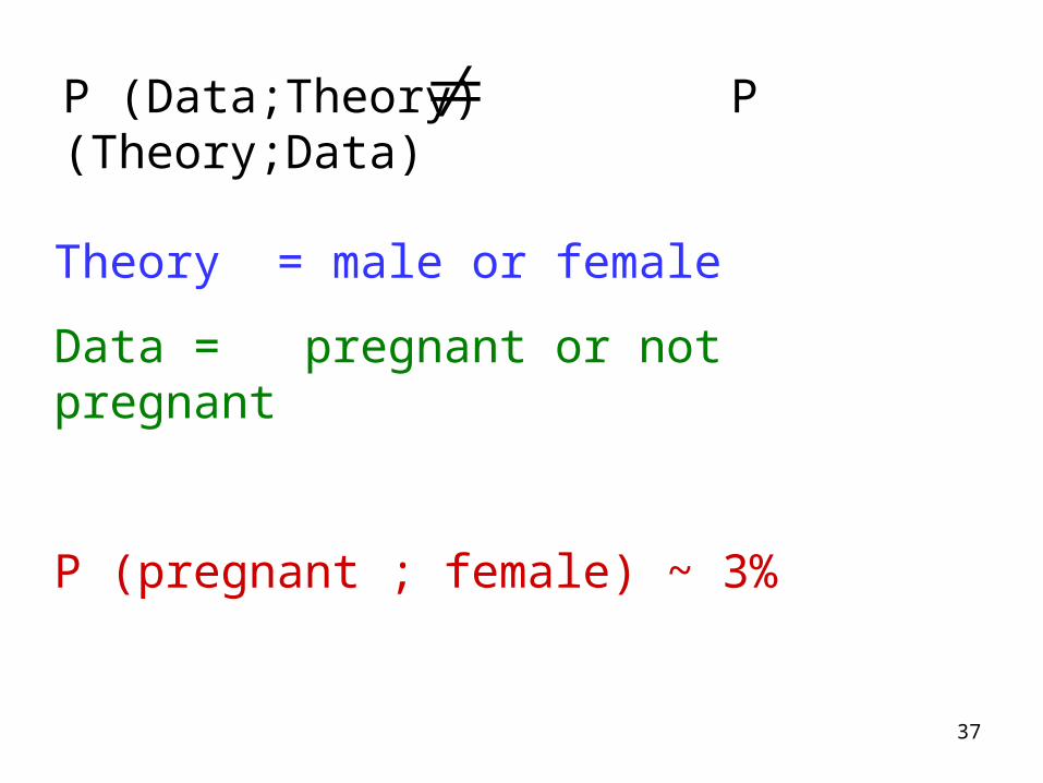
P (Data;Theory) P (Theory;Data)

Theory = male or female

Data = pregnant or not pregnant

P (pregnant ; female) ~ 3%

38

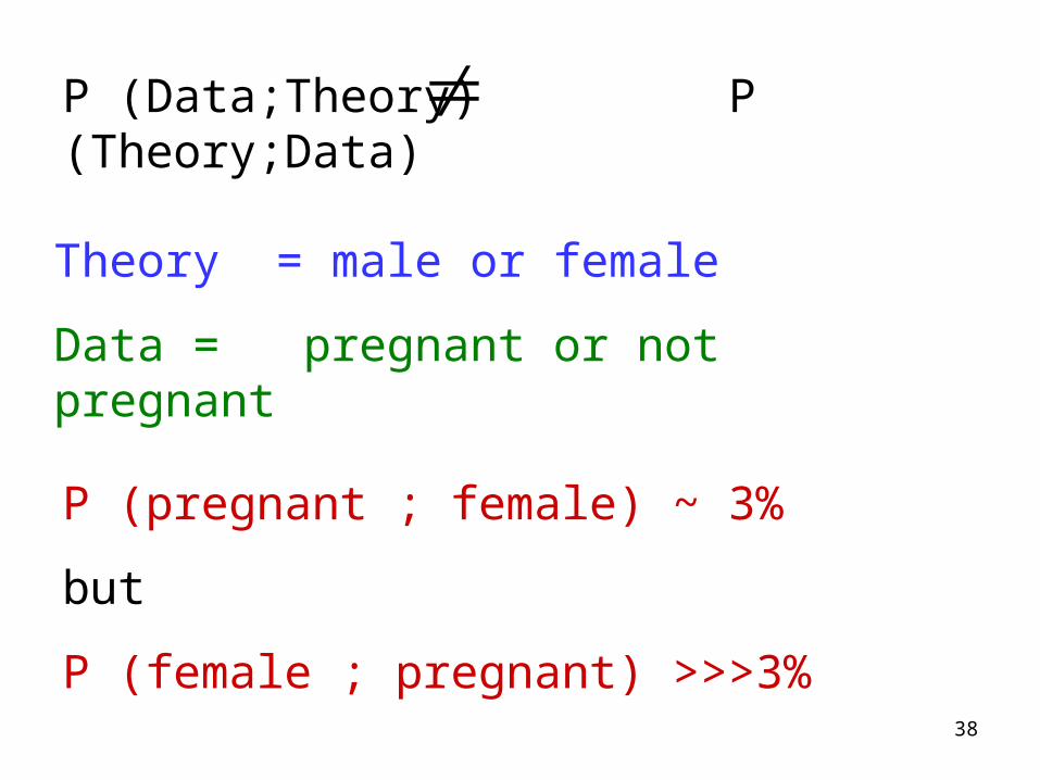
P (Data;Theory) P (Theory;Data)

Theory = male or female

Data = pregnant or not pregnant

P (pregnant ; female) ~ 3%

but

P (female ; pregnant) >>>3%

39

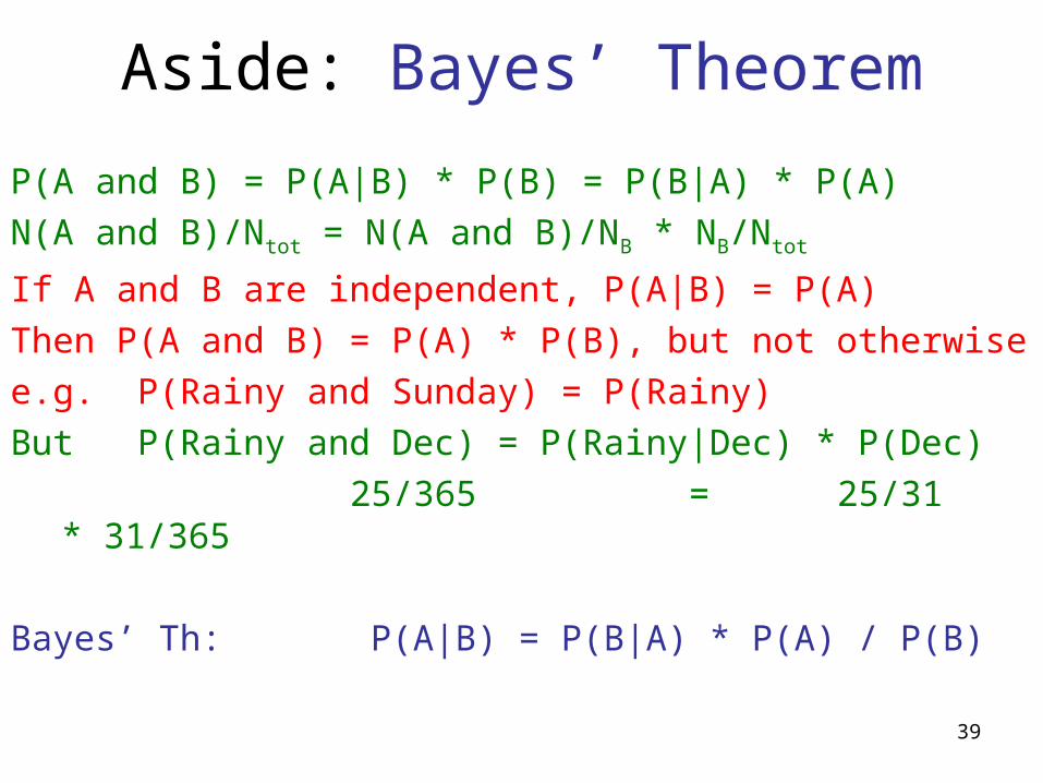
Aside: Bayes’ Theorem

P(A and B) = P(A|B) * P(B) = P(B|A) * P(A)

N(A and B)/Ntot = N(A and B)/NB * NB/Ntot

If A and B are independent, P(A|B) = P(A)

Then P(A and B) = P(A) * P(B), but not otherwise

e.g. P(Rainy and Sunday) = P(Rainy)

But P(Rainy and Dec) = P(Rainy|Dec) * P(Dec)

25/365 = 25/31 * 31/365

Bayes’ Th: P(A|B) = P(B|A) * P(A) / P(B)

40

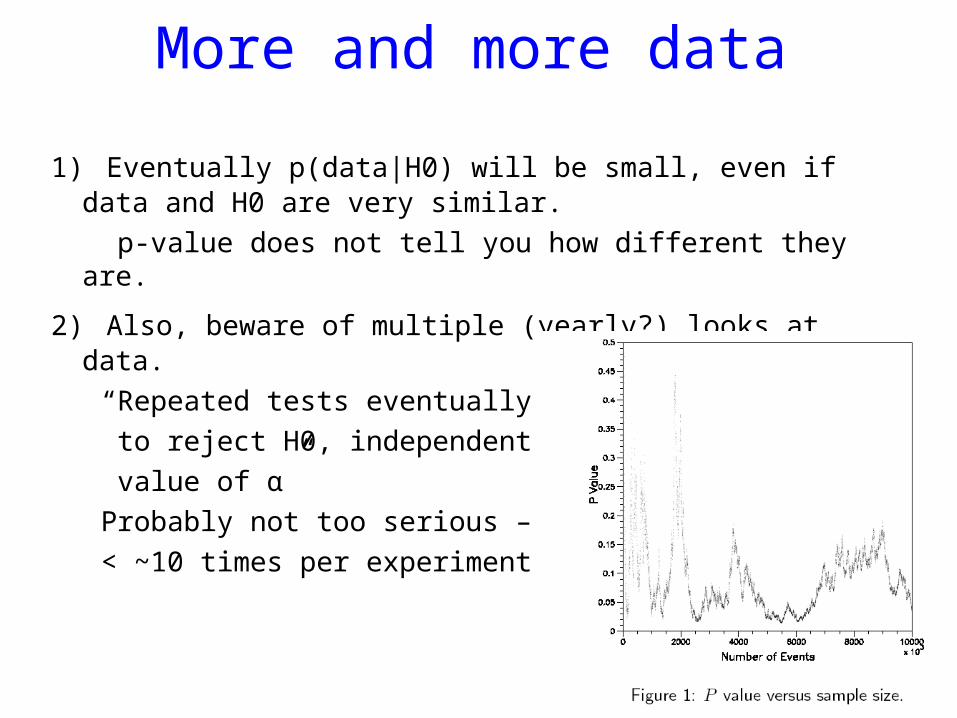
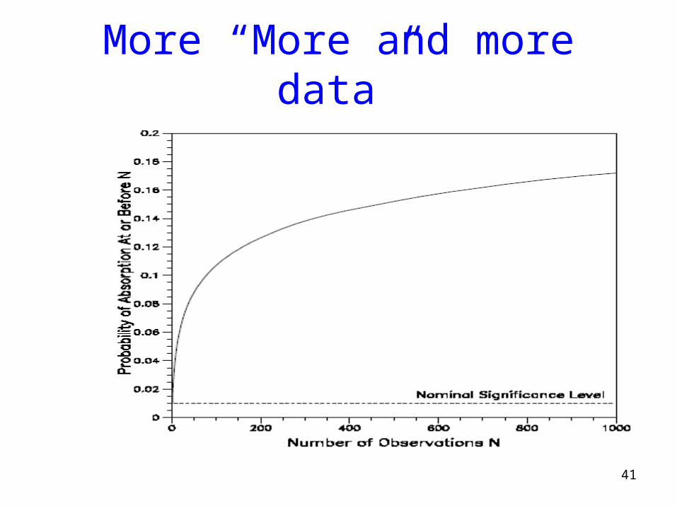
More and more data

1) Eventually p(data|H0) will be small, even if data and H0 are very similar.

p-value does not tell you how different they are.

2) Also, beware of multiple (yearly?) looks at data.

“Repeated tests eventually sure

to reject H0, independent of

value of α”

Probably not too serious –

< ~10 times per experiment.

41

More “More and more data”

42

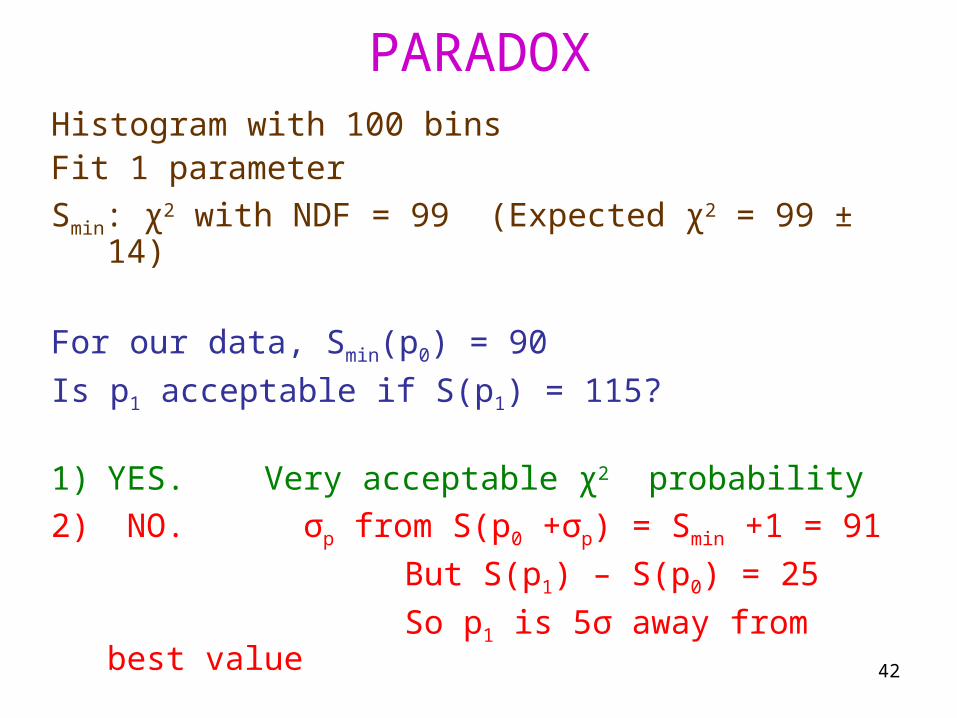
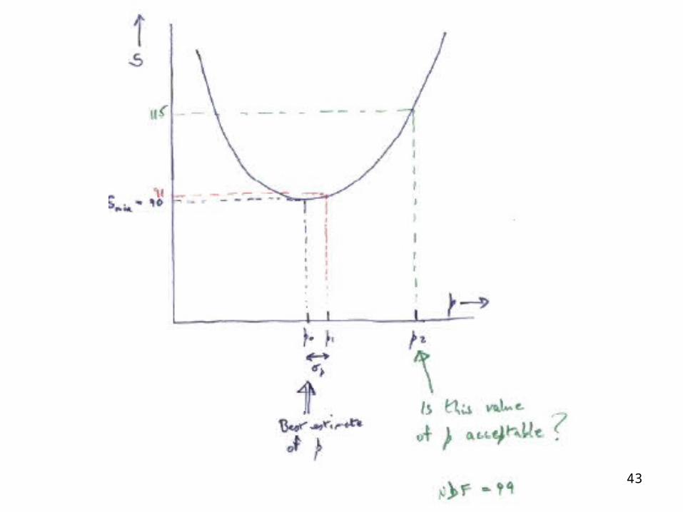
PARADOXHistogram with 100 binsFit 1 parameter

Smin: χ2 with NDF = 99 (Expected χ2 = 99 ± 14)

For our data, Smin(p0) = 90

Is p1 acceptable if S(p1) = 115?

1) YES. Very acceptable χ2 probability

2) NO. σp from S(p0 +σp) = Smin +1 = 91

But S(p1) – S(p0) = 25

So p1 is 5σ away from best value

43

45

46

47

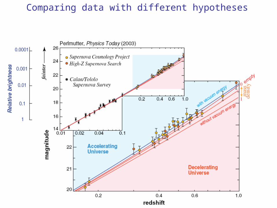
Comparing data with different hypotheses

48

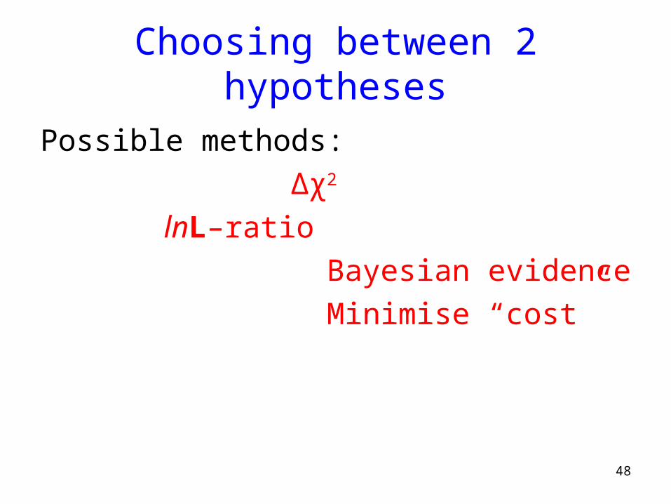
Choosing between 2 hypotheses

Possible methods:

Δχ2

lnL–ratio

Bayesian evidence

Minimise “cost”

49

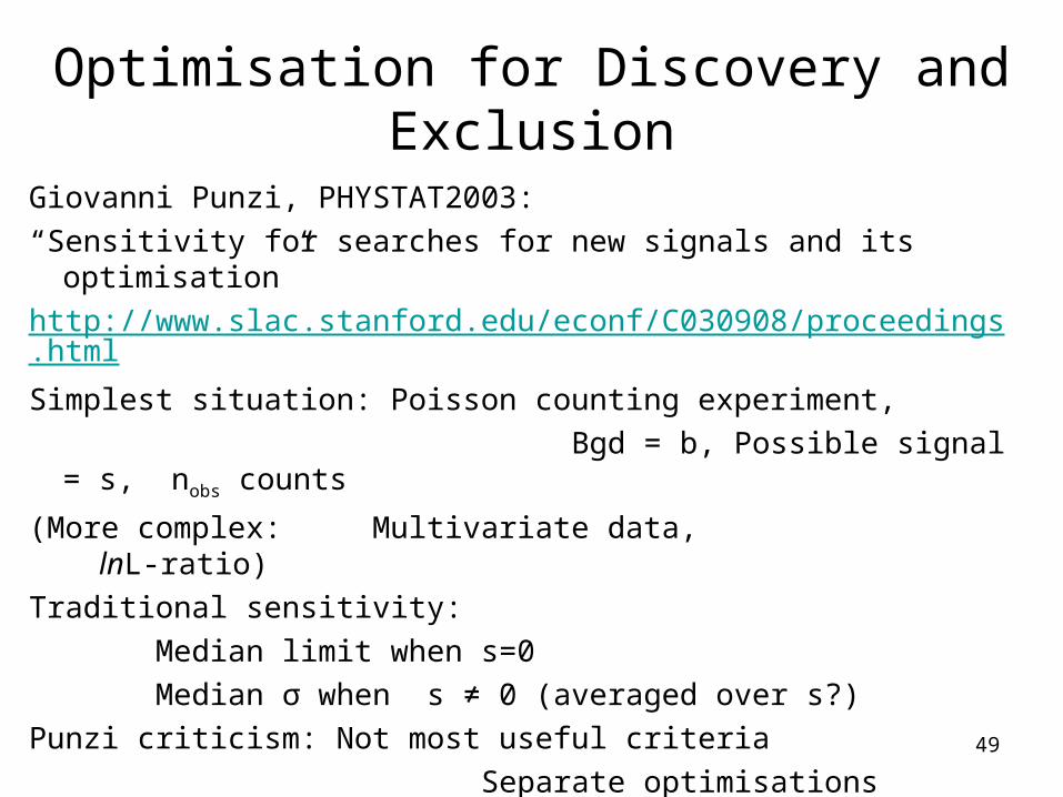
Optimisation for Discovery and Exclusion

Giovanni Punzi, PHYSTAT2003:

“Sensitivity for searches for new signals and its optimisation”

http://www.slac.stanford.edu/econf/C030908/proceedings.html

Simplest situation: Poisson counting experiment,

Bgd = b, Possible signal = s, nobs counts

(More complex: Multivariate data, lnL-ratio)

Traditional sensitivity:

Median limit when s=0

Median σ when s ≠ 0 (averaged over s?)

Punzi criticism: Not most useful criteria

Separate optimisations

50

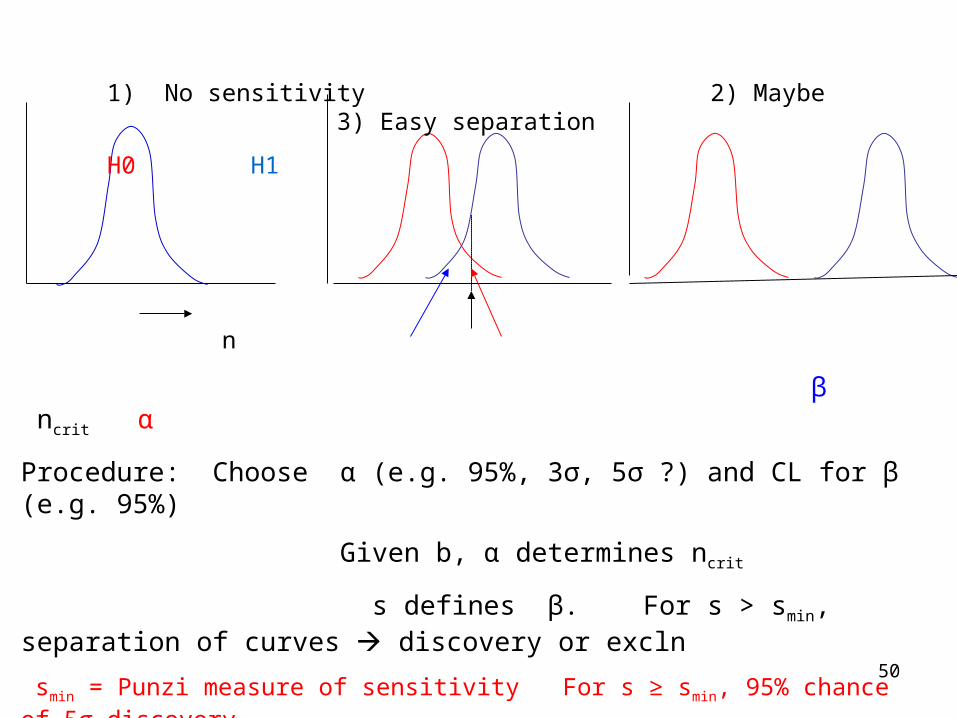
1) No sensitivity 2) Maybe 3) Easy separation

H0 H1

n

β ncrit α

Procedure: Choose α (e.g. 95%, 3σ, 5σ ?) and CL for β (e.g. 95%)

Given b, α determines ncrit

s defines β. For s > smin, separation of curves discovery or excln

smin = Punzi measure of sensitivity For s ≥ smin, 95% chance of 5σ discovery

Optimise cuts for smallest smin

Now data: If nobs ≥ ncrit, discovery at level α

If nobs < ncrit, no discovery. If βobs < 1 – CL, exclude H1

51

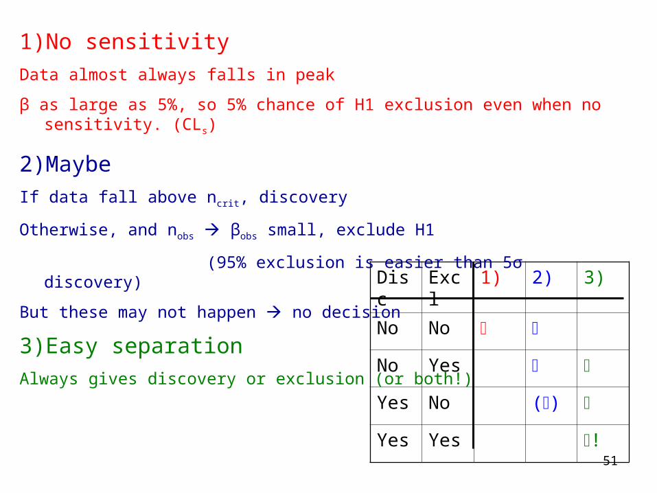
Disc Excl 1) 2) 3)

No No

No Yes

Yes No ()

Yes Yes !

1) No sensitivity

Data almost always falls in peak

β as large as 5%, so 5% chance of H1 exclusion even when no sensitivity. (CLs)

2) Maybe

If data fall above ncrit, discovery

Otherwise, and nobs βobs small, exclude H1

(95% exclusion is easier than 5σ discovery)

But these may not happen no decision

3) Easy separation

Always gives discovery or exclusion (or both!)

52

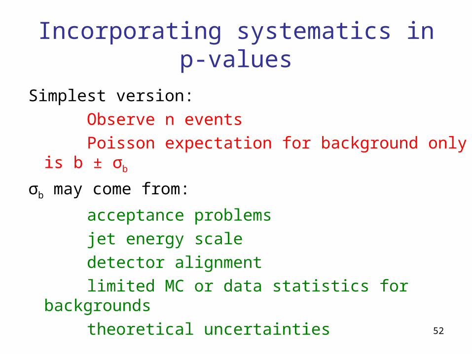
Incorporating systematics in p-values

Simplest version:

Observe n events

Poisson expectation for background only is b ± σb

σb may come from:

acceptance problems

jet energy scale

detector alignment

limited MC or data statistics for backgrounds

theoretical uncertainties

53

Luc Demortier,“p-values: What they are and how we use them”, CDF memo June 2006

http://www-cdfd.fnal.gov/~luc/statistics/cdf0000.ps

Includes discussion of several ways of incorporating nuisance parameters

Desiderata:

Uniformity of p-value (averaged over ν, or for each ν?)

p-value increases as σν increases

Generality

Maintains power for discovery

54

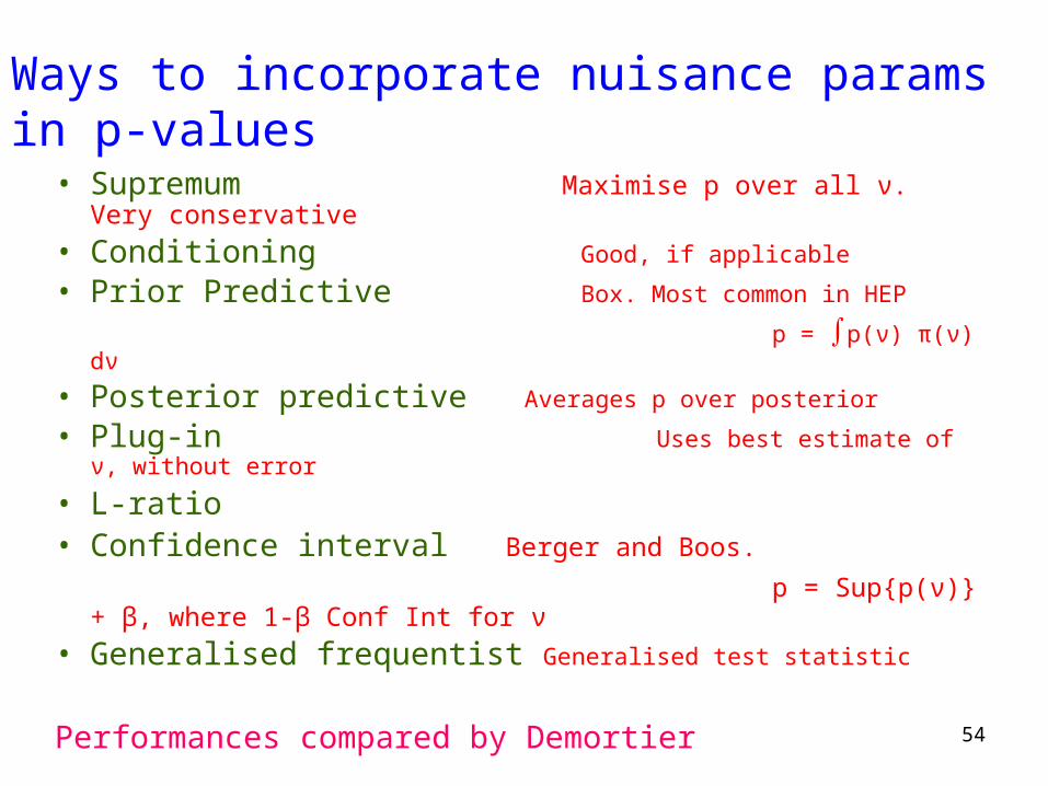
• Supremum Maximise p over all ν. Very conservative

• Conditioning Good, if applicable

• Prior Predictive Box. Most common in HEP

p = ∫p(ν) π(ν) dν

• Posterior predictive Averages p over posterior

• Plug-in Uses best estimate of ν, without error

• L-ratio• Confidence interval Berger and Boos. p = Sup{p(ν)} + β, where 1-β Conf Int for ν

• Generalised frequentist Generalised test statistic

Performances compared by Demortier

Ways to incorporate nuisance params in p-values

55

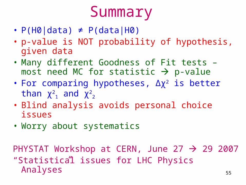
Summary• P(H0|data) ≠ P(data|H0)• p-value is NOT probability of hypothesis, given

data• Many different Goodness of Fit tests – most need

MC for statistic p-value• For comparing hypotheses, Δχ2 is better than χ2

1 and χ2

2

• Blind analysis avoids personal choice issues• Worry about systematics

PHYSTAT Workshop at CERN, June 27 29 2007“Statistical issues for LHC Physics Analyses”

56

Final message

Send interesting statistical issues to

l.lyons@physics.ox.ac.uk