1 Overview

In this work, we describe the basic usage of the hierarchical Bayesian formulation of the ctsem(Driver, Oud & Voelkle, 2017) software for continuous-time dynamic modelling in R (R Core Team,2014). This formulation, described in detail in Driver and Voelkle (in press), offers advantages overwhat could be considered more typical dynamic modelling approaches, such as vector autoregressivemodels or latent change score models. The two main advantages relate to the handling of time, andthe treatment of individual differences. Time information is explicitly incorporated into the model,such that predictions from one measurement to another relate exactly to the amount of time thathas passed, rather than simply the number of measurements, as is typical in discrete-time models.When the time interval between all measurements are equal, there is an exact relationship betweenthe discrete and continuous time form, but when they differ, the continuous-time form is typicallymore appropriate. For more on continuous-time models, see Oud and Jansen (2000), Singer (1993),Voelkle and Oud (2013). With respect to individual differences, the hierarchical Bayesian approachallows for individual variation across all model parameters, while still making full use of the datafrom all subjects. This has the result that individual specific parameter estimates may be obtainedwith far fewer time points than would be required by single-subject time-series type modellingapproaches. For more on hierarchical Bayesian models, see Gelman, Carlin, Stern and Rubin(2014).This document is structured such that we first briefly describe the continuous time dynamic modelgoverning within subject dynamics, and the hierarchical model governing the distribution of subjectlevel parameters. These aspects are covered in detail in Driver and Voelkle (in press). Following,we walk through installing the ctsem software, setting up a data structure, specifying and fittingthe model, followed by summary and plotting functions. Some details on additional complexity arethen provided, including an example model with a more complex dynamic structure, a discussion ofthe various options for incorporating stationarity assumptions into the model, and a walk-throughof the various transformations involved in the model.

1.1 Subject Level Latent Dynamic model

This section describes the subject level model characterising the system dynamics and measurementproperties. Although we do not describe it explicitly, the corresponding discrete time autoregressive/ moving average models can be specified and use the same set of parameter matrices we describe.

1.2 Subject level latent dynamic model

The subject level dynamics are described by the following stochastic differential equation:

dη(t) =(

Aη(t) + b + Mχ(t))

dt+ GdW(t) (1)

Vector η(t) ∈ Rv represents the state of the latent processes at time t. The matrix A ∈ Rv×v

(DRIFT) represents the drift matrix, with auto effects on the diagonal and cross effects on theoff-diagonals characterizing the temporal dynamics of the processes.The continuous time intercept vector b ∈ Rv (CINT), in combination with A, determines thelong-term level at which the processes fluctuate around.

1

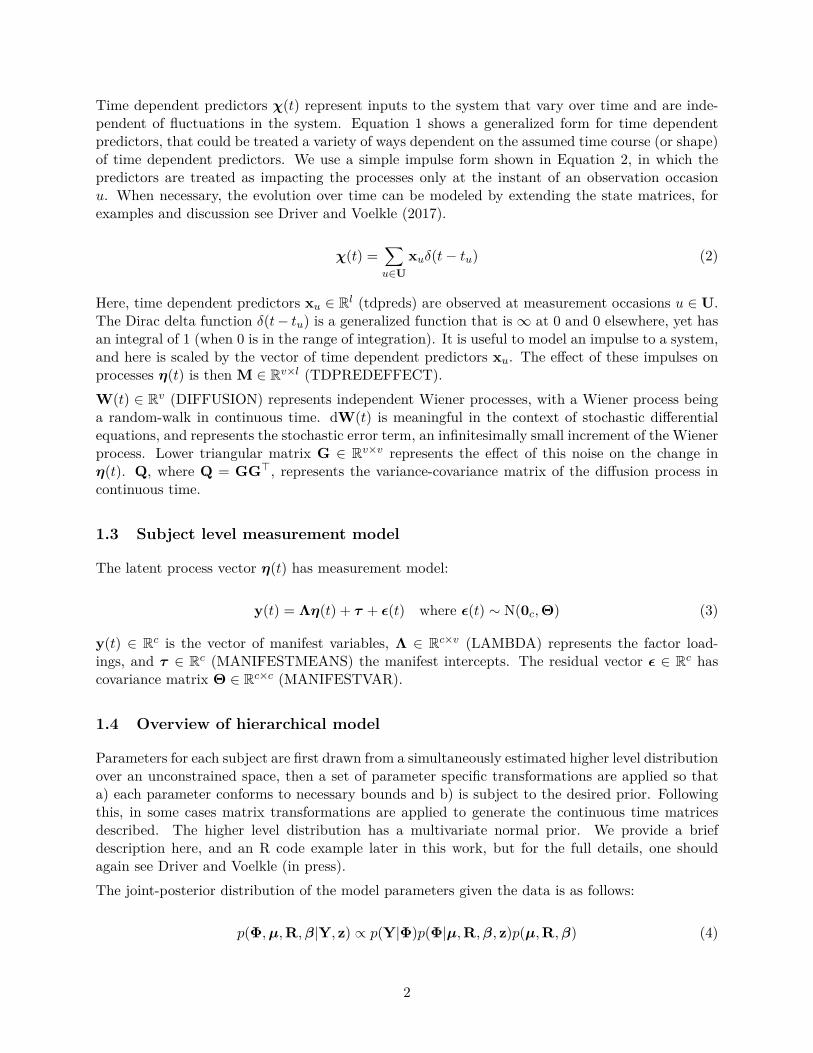
Time dependent predictors χ(t) represent inputs to the system that vary over time and are inde-pendent of fluctuations in the system. Equation 1 shows a generalized form for time dependentpredictors, that could be treated a variety of ways dependent on the assumed time course (or shape)of time dependent predictors. We use a simple impulse form shown in Equation 2, in which thepredictors are treated as impacting the processes only at the instant of an observation occasionu. When necessary, the evolution over time can be modeled by extending the state matrices, forexamples and discussion see Driver and Voelkle (2017).

χ(t) =∑u∈U

xuδ(t− tu) (2)

Here, time dependent predictors xu ∈ Rl (tdpreds) are observed at measurement occasions u ∈ U.The Dirac delta function δ(t− tu) is a generalized function that is ∞ at 0 and 0 elsewhere, yet hasan integral of 1 (when 0 is in the range of integration). It is useful to model an impulse to a system,and here is scaled by the vector of time dependent predictors xu. The effect of these impulses onprocesses η(t) is then M ∈ Rv×l (TDPREDEFFECT).W(t) ∈ Rv (DIFFUSION) represents independent Wiener processes, with a Wiener process beinga random-walk in continuous time. dW(t) is meaningful in the context of stochastic differentialequations, and represents the stochastic error term, an infinitesimally small increment of the Wienerprocess. Lower triangular matrix G ∈ Rv×v represents the effect of this noise on the change inη(t). Q, where Q = GG>, represents the variance-covariance matrix of the diffusion process incontinuous time.

1.3 Subject level measurement model

The latent process vector η(t) has measurement model:

y(t) = Λη(t) + τ + ε(t) where ε(t) ∼ N(0c,Θ) (3)

y(t) ∈ Rc is the vector of manifest variables, Λ ∈ Rc×v (LAMBDA) represents the factor load-ings, and τ ∈ Rc (MANIFESTMEANS) the manifest intercepts. The residual vector ε ∈ Rc hascovariance matrix Θ ∈ Rc×c (MANIFESTVAR).

1.4 Overview of hierarchical model

Parameters for each subject are first drawn from a simultaneously estimated higher level distributionover an unconstrained space, then a set of parameter specific transformations are applied so thata) each parameter conforms to necessary bounds and b) is subject to the desired prior. Followingthis, in some cases matrix transformations are applied to generate the continuous time matricesdescribed. The higher level distribution has a multivariate normal prior. We provide a briefdescription here, and an R code example later in this work, but for the full details, one shouldagain see Driver and Voelkle (in press).The joint-posterior distribution of the model parameters given the data is as follows:

p(Φ,µ,R,β|Y, z) ∝ p(Y|Φ)p(Φ|µ,R,β, z)p(µ,R,β) (4)

2

Subject specific parameters Φi are determined in the following manner:

Φi = tform(µ+ Rhi + βzi

)(5)

hi ∼ N(0, 1) (6)

µ ∼ N(0, 1) (7)

β ∼ N(0, 1) (8)

Φi ∈ Rs is the s length vector of parameters for the dynamic and measurement models of subjecti. µ ∈ Rs parameterizes the means of the raw population distributions of subject level parameters.R ∈ Rs×s is the matrix square root of the raw population distribution covariance matrix, para-meterizing the effect of subject specific deviations hi ∈ Rs on Φi. β ∈ Rs×w is the raw effect oftime independent predictors zi ∈ Rw on Φi, where w is the number of time independent predictors.Yi contains all the data for subject i used in the subject level model – y (process related meas-urements) and x (time dependent predictors). zi contains time independent predictors data forsubject i. tform is an operator that applies a transform to each value of the vector it is applied to.The specific transform depends on which subject level parameter matrix the value belongs to, andthe position in that matrix.At a number of points, we will refer to the parameters prior to the tform function as ’raw’ para-meters. So for instance ‘raw population standard deviation’ would refer to a diagonal entry of R,and ‘raw individual parameters for subject i’ would refer to µ + Rhi + βzi. In contrast, withoutthe ‘raw’ prefix, ‘population means’ would refer to tform(µ), and would typically reflect values theuser is more likely to be interested in, such as the continuous time drift parameters.

1.5 Install software and prepare data

Install ctsem software within R:

install.packages("ctsem")library("ctsem")

Prepare data in long format, each row containing one time point of data for one subject. We needa subject id column, named by default "id", though this can be changed in the model specification.Some of the outputs are simpler to interpret if subject id is a sequence of integers from 1 to thenumber of subjects, but this is not a requirement. We also need a time column "time", containingpositive numeric values for time, columns for manifest variables (the names of which must be givenin the next step using ctModel), columns for time dependent predictors (these vary over time buthave no model estimated and are assumed to impact latent processes instantly), and columns fortime independent predictors (which predict the subject level parameters, that are themselves timeinvariant – thus the values for a particular time independent predictor must be the same across allobservations of a particular subject).

id time Y1 Y2 TD1 TI1 TI2 TI3[1,] 1 1.877 0.2975 -4.728 0 -0.701 1.257 -0.361[2,] 1 3.608 6.5180 -2.518 0 -0.701 1.257 -0.361[3,] 1 4.765 3.2376 0.755 0 -0.701 1.257 -0.361[4,] 1 15.385 0.0471 -7.386 0 -0.701 1.257 -0.361

3

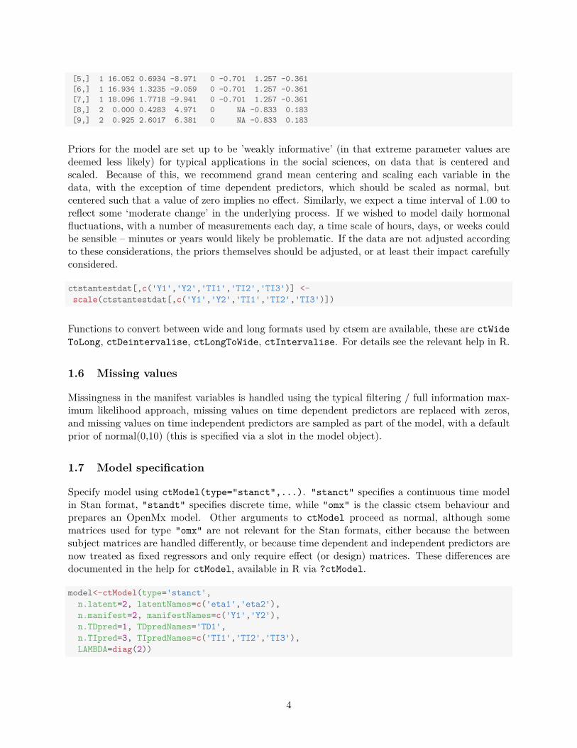
[5,] 1 16.052 0.6934 -8.971 0 -0.701 1.257 -0.361[6,] 1 16.934 1.3235 -9.059 0 -0.701 1.257 -0.361[7,] 1 18.096 1.7718 -9.941 0 -0.701 1.257 -0.361[8,] 2 0.000 0.4283 4.971 0 NA -0.833 0.183[9,] 2 0.925 2.6017 6.381 0 NA -0.833 0.183

Priors for the model are set up to be ’weakly informative’ (in that extreme parameter values aredeemed less likely) for typical applications in the social sciences, on data that is centered andscaled. Because of this, we recommend grand mean centering and scaling each variable in thedata, with the exception of time dependent predictors, which should be scaled as normal, butcentered such that a value of zero implies no effect. Similarly, we expect a time interval of 1.00 toreflect some ‘moderate change’ in the underlying process. If we wished to model daily hormonalfluctuations, with a number of measurements each day, a time scale of hours, days, or weeks couldbe sensible – minutes or years would likely be problematic. If the data are not adjusted accordingto these considerations, the priors themselves should be adjusted, or at least their impact carefullyconsidered.

ctstantestdat[,c('Y1','Y2','TI1','TI2','TI3')] <-scale(ctstantestdat[,c('Y1','Y2','TI1','TI2','TI3')])

Functions to convert between wide and long formats used by ctsem are available, these are ctWideToLong, ctDeintervalise, ctLongToWide, ctIntervalise. For details see the relevant help in R.

1.6 Missing values

Missingness in the manifest variables is handled using the typical filtering / full information max-imum likelihood approach, missing values on time dependent predictors are replaced with zeros,and missing values on time independent predictors are sampled as part of the model, with a defaultprior of normal(0,10) (this is specified via a slot in the model object).

1.7 Model specification

Specify model using ctModel(type="stanct",...). "stanct" specifies a continuous time modelin Stan format, "standt" specifies discrete time, while "omx" is the classic ctsem behaviour andprepares an OpenMx model. Other arguments to ctModel proceed as normal, although somematrices used for type "omx" are not relevant for the Stan formats, either because the betweensubject matrices are handled differently, or because time dependent and independent predictors arenow treated as fixed regressors and only require effect (or design) matrices. These differences aredocumented in the help for ctModel, available in R via ?ctModel.

model<-ctModel(type='stanct',n.latent=2, latentNames=c('eta1','eta2'),n.manifest=2, manifestNames=c('Y1','Y2'),n.TDpred=1, TDpredNames='TD1',n.TIpred=3, TIpredNames=c('TI1','TI2','TI3'),LAMBDA=diag(2))

4

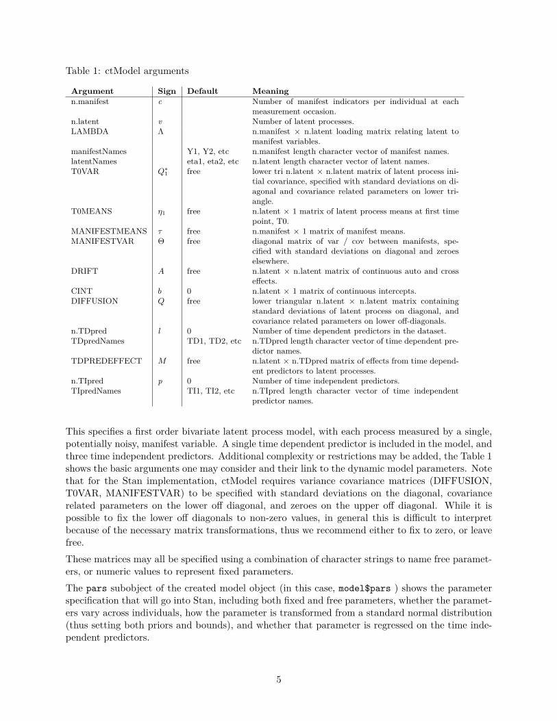
Table 1: ctModel arguments

Argument Sign Default Meaningn.manifest c Number of manifest indicators per individual at each

measurement occasion.n.latent v Number of latent processes.LAMBDA Λ n.manifest × n.latent loading matrix relating latent to

manifest variables.manifestNames Y1, Y2, etc n.manifest length character vector of manifest names.latentNames eta1, eta2, etc n.latent length character vector of latent names.T0VAR Q∗

1 free lower tri n.latent × n.latent matrix of latent process ini-tial covariance, specified with standard deviations on di-agonal and covariance related parameters on lower tri-angle.

T0MEANS η1 free n.latent × 1 matrix of latent process means at first timepoint, T0.

MANIFESTMEANS τ free n.manifest × 1 matrix of manifest means.MANIFESTVAR Θ free diagonal matrix of var / cov between manifests, spe-

cified with standard deviations on diagonal and zeroeselsewhere.

DRIFT A free n.latent × n.latent matrix of continuous auto and crosseffects.

CINT b 0 n.latent × 1 matrix of continuous intercepts.DIFFUSION Q free lower triangular n.latent × n.latent matrix containing

standard deviations of latent process on diagonal, andcovariance related parameters on lower off-diagonals.

n.TDpred l 0 Number of time dependent predictors in the dataset.TDpredNames TD1, TD2, etc n.TDpred length character vector of time dependent pre-

dictor names.TDPREDEFFECT M free n.latent × n.TDpred matrix of effects from time depend-

ent predictors to latent processes.n.TIpred p 0 Number of time independent predictors.TIpredNames TI1, TI2, etc n.TIpred length character vector of time independent

predictor names.

This specifies a first order bivariate latent process model, with each process measured by a single,potentially noisy, manifest variable. A single time dependent predictor is included in the model, andthree time independent predictors. Additional complexity or restrictions may be added, the Table 1shows the basic arguments one may consider and their link to the dynamic model parameters. Notethat for the Stan implementation, ctModel requires variance covariance matrices (DIFFUSION,T0VAR, MANIFESTVAR) to be specified with standard deviations on the diagonal, covariancerelated parameters on the lower off diagonal, and zeroes on the upper off diagonal. While it ispossible to fix the lower off diagonals to non-zero values, in general this is difficult to interpretbecause of the necessary matrix transformations, thus we recommend either to fix to zero, or leavefree.These matrices may all be specified using a combination of character strings to name free paramet-ers, or numeric values to represent fixed parameters.The pars subobject of the created model object (in this case, model$pars ) shows the parameterspecification that will go into Stan, including both fixed and free parameters, whether the paramet-ers vary across individuals, how the parameter is transformed from a standard normal distribution(thus setting both priors and bounds), and whether that parameter is regressed on the time inde-pendent predictors.

5

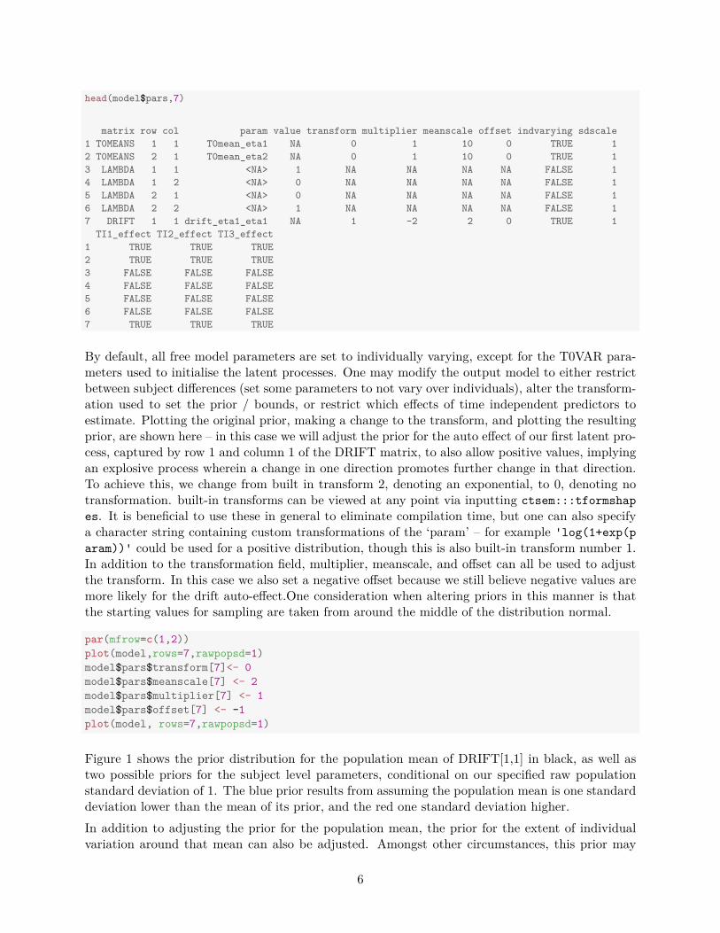
head(model$pars,7)

matrix row col param value transform multiplier meanscale offset indvarying sdscale1 T0MEANS 1 1 T0mean_eta1 NA 0 1 10 0 TRUE 12 T0MEANS 2 1 T0mean_eta2 NA 0 1 10 0 TRUE 13 LAMBDA 1 1 <NA> 1 NA NA NA NA FALSE 14 LAMBDA 1 2 <NA> 0 NA NA NA NA FALSE 15 LAMBDA 2 1 <NA> 0 NA NA NA NA FALSE 16 LAMBDA 2 2 <NA> 1 NA NA NA NA FALSE 17 DRIFT 1 1 drift_eta1_eta1 NA 1 -2 2 0 TRUE 1

TI1_effect TI2_effect TI3_effect1 TRUE TRUE TRUE2 TRUE TRUE TRUE3 FALSE FALSE FALSE4 FALSE FALSE FALSE5 FALSE FALSE FALSE6 FALSE FALSE FALSE7 TRUE TRUE TRUE

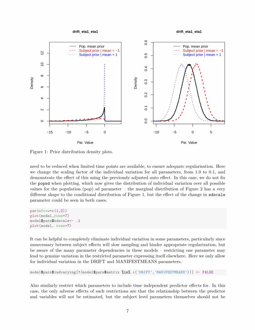
By default, all free model parameters are set to individually varying, except for the T0VAR para-meters used to initialise the latent processes. One may modify the output model to either restrictbetween subject differences (set some parameters to not vary over individuals), alter the transform-ation used to set the prior / bounds, or restrict which effects of time independent predictors toestimate. Plotting the original prior, making a change to the transform, and plotting the resultingprior, are shown here – in this case we will adjust the prior for the auto effect of our first latent pro-cess, captured by row 1 and column 1 of the DRIFT matrix, to also allow positive values, implyingan explosive process wherein a change in one direction promotes further change in that direction.To achieve this, we change from built in transform 2, denoting an exponential, to 0, denoting notransformation. built-in transforms can be viewed at any point via inputting ctsem:::tformshapes. It is beneficial to use these in general to eliminate compilation time, but one can also specifya character string containing custom transformations of the ‘param’ – for example 'log(1+exp(param))' could be used for a positive distribution, though this is also built-in transform number 1.In addition to the transformation field, multiplier, meanscale, and offset can all be used to adjustthe transform. In this case we also set a negative offset because we still believe negative values aremore likely for the drift auto-effect.One consideration when altering priors in this manner is thatthe starting values for sampling are taken from around the middle of the distribution normal.

par(mfrow=c(1,2))plot(model,rows=7,rawpopsd=1)model$pars$transform[7]<- 0model$pars$meanscale[7] <- 2model$pars$multiplier[7] <- 1model$pars$offset[7] <- -1plot(model, rows=7,rawpopsd=1)

Figure 1 shows the prior distribution for the population mean of DRIFT[1,1] in black, as well astwo possible priors for the subject level parameters, conditional on our specified raw populationstandard deviation of 1. The blue prior results from assuming the population mean is one standarddeviation lower than the mean of its prior, and the red one standard deviation higher.In addition to adjusting the prior for the population mean, the prior for the extent of individualvariation around that mean can also be adjusted. Amongst other circumstances, this prior may

6

−15 −10 −5 0

02

46

810

12

drift_eta1_eta1

Par. Value

Den

sity

Pop. mean priorSubject prior | mean = −1Subject prior | mean = 1

−10 −5 0 5

0.0

0.1

0.2

0.3

0.4

0.5

0.6

drift_eta1_eta1

Par. Value

Den

sity

Pop. mean priorSubject prior | mean = −1Subject prior | mean = 1

Figure 1: Prior distribution density plots.

need to be reduced when limited time points are available, to ensure adequate regularisation. Herewe change the scaling factor of the individual variation for all parameters, from 1.0 to 0.1, anddemonstrate the effect of this using the previously adjusted auto effect. In this case, we do not fixthe popsd when plotting, which now gives the distribution of individual variation over all possiblevalues for the population (pop) sd parameter – the marginal distribution of Figure 2 has a verydifferent shape to the conditional distribution of Figure 1, but the effect of the change in sdscaleparameter could be seen in both cases.

par(mfrow=c(1,2))plot(model,rows=7)model$pars$sdscale<- .1plot(model, rows=7)

It can be helpful to completely eliminate individual variation in some parameters, particularly sinceunnecessary between subject effects will slow sampling and hinder appropriate regularization, butbe aware of the many parameter dependencies in these models – restricting one parameter maylead to genuine variation in the restricted parameter expressing itself elsewhere. Here we only allowfor individual variation in the DRIFT and MANIFESTMEANS parameters.

model$pars$indvarying[!(model$pars$matrix %in% c('DRIFT','MANIFESTMEANS'))] <- FALSE

Also similarly restrict which parameters to include time independent predictor effects for. In thiscase, the only adverse effects of such restrictions are that the relationship between the predictorand variables will not be estimated, but the subject level parameters themselves should not be

7

−15 −10 −5 0 5 10 15

01

23

4

drift_eta1_eta1

Par. Value

Den

sity

Pop. mean priorSubject prior | mean = −1Subject prior | mean = 1

−15 −10 −5 0 5 10 15

01

23

4

drift_eta1_eta1

Par. Value

Den

sity

Pop. mean priorSubject prior | mean = −1Subject prior | mean = 1

Figure 2: Prior distribution density plots of auto-effects, with default (left) and adjusted (right)scale parameter for population standard deviation.

very different, as they are still freely estimated. Note that such effects can only be estimated forparameters specified as individually varying – in case one particularly wished to model a covariateeffect without allowing for residual variation, this could be approximated by setting the parameterto indvarying, but putting a very small sdscale value for the parameter. Here, we first restrictthe tipredeffects on all parameters, and free them only for the drift parameters.

model$pars[,c('TI1_effect','TI2_effect','TI3_effect')] <- FALSEmodel$pars[model$pars$matrix == 'DRIFT',

c('TI1_effect','TI2_effect','TI3_effect')] <- TRUE

1.8 Model fitting

Once model specification is complete, the model is fit to the data using the ctStanFit function asshown in the following example. Depending on the data, model, and number of iterations requested,this can take anywhere from a few minutes to days. Current experience suggests 300 iterations isoften enough to get an idea of what is going on, but more may be necessary for robust inference,but this is highly dependent on the specifics. For the sake of speed for this example we only samplefor 300 iterations, with a max treedepth of the Hamiltonian sampler reduced from the default of10 to 6. With these settings the fit should take only a minute or two, but is unlikely adequate forinference!. Those that wish to try out the functions without waiting, can simply use the alreadyexisting ctstantestfit object with the relevant functions (the code for this is commented out).The dataset specified here is built-in to the ctsem package, and available whenever ctsem is loadedin R.

8

fit<-ctStanFit(datalong = ctstantestdat, ctstanmodel = model, iter=200,control=list(max_treedepth=6), chains=2, plot=FALSE)

# fit <- ctstantestfit

The plot argument allows for plotting of sampling chains in real time, which is useful for slow modelsto ensure that sampling is proceeding in a functional manner. Models with many parameters (e.g.,many subjects and all parameters varying over subject) may be too taxing for the plotting functionto handle smoothly - we have had success with up to around 4000 parameters.

1.9 Summary

After fitting, the summary function may be used on the fit object, which returns details regardingthe population mean parameters, population standard deviation parameters, population correla-tions, and the effect parameters of time independent predictors. Additionally, summary outputsa range of matrices regarding correlations between subject level parameters. rawpopcorr_meansreports the posterior mean of the correlation between raw (not yet transformed from the standardnormal scale) parameters. rawpopcorr_sd reports the standard deviation of these parameters.

summary(fit,timeinterval = 1)

In the summary output, the free population mean parameters under $popmeans are likely one ofthe main points of interest. They are returned in the same form that they are input to ctModel- that is, covariance matrix related parameters are in the form of either standard deviations or atransformed correlation parameter. Because the latter is difficult to interpret, various parametermatrices are also returned in the $parmatrices section of the summary. The discrete time matricesreported here (prefixed by dt) are by default from a time interval of 1, but this can be changed.Asymptotic matrices – those for a time interval of infinity – are also output in some cases, andprefixed by asym. Covariance related matrices are reported in covariance form, except where thesuffix cor is added to indicate correlations.The function ctStanContinuousPars can be used to return the continuous time parameter matricesin actual matrix form, for specific subjects, or groups of subjects. By default the median is calcu-lated, but the function that aggregates over samples can be changed as desired. In the followingcode, the 97.5% quantile is returned, for subject 3.

ctStanContinuousPars(fit,subjects = 3, calcfunc = quantile, calcfuncargs = list(probs=.975))

Note that subject 3 refers to the third subject in the data, not any particular identifier specified inthe subject id column. The mapping of subject id to the internal sequential integer representationcan be found via fit$setup$idmap . If a vector of subjects is specified, or the string 'all' is used,multiple subjects are aggregated over.

1.10 Plotting

The plot function outputs a sequence of plots, all generated by specific functions. The name of thespecific function appears in a message in the R console, checking the help for each specific functionand running them separately will allow more customization of plots. Some of the plots, such as

9

the trace, density, and interval, are generated by the relevant rstan function and are hopefully selfexplanatory. The plots specific to the hierarchical continuous time dynamic model are as follows:

ctStanDiscretePars(fit, plot=TRUE, indices = 'CR', subjects = 'all')

0 2 4 6 8 10

−1.

5−

0.5

0.0

0.5

1.0

1.5

Regression coefficients

Time interval

Val

ue

eta2_eta1eta1_eta2

Figure 3: Discrete-time cross-effect dynamics of the estimated system for a range of timeintervals, with 95% credible intervals.

Figure 3 shows the dynamic regression coefficients (between latent states at different time points)that are implied by the model for particular time intervals, as well as the uncertainty (default is95% credible interval) of these coefficients. In this case the estimates are of the cross regressioneffects, obtained by sampling from all subjects data, but specific subjects, as well as specific indicesof the effects (e.g., indices = ’AR’ or indices = rbind(c(2,1))’ can be specified.The relation between posteriors and priors for variables of interest can also be plotted as follows –note that the rows argument of the shown code is not necessary, but if only particular parameterplots are desired the rows corresponding to specific parameters of fit$setup$popsetup can bespecified.

ctStanPlotPost(obj = fit, rows=3)

Shown in Figure 4 are approximate density plots based on the post-warmup samples drawn. Foreach parameter that has individual variation specified, three plots are shown. These are the popu-lation mean posterior compared to the prior, the posterior versus prior distribution of subject levelparameters along with the population mean prior, and then the population standard deviationposterior compared to the prior.

10

−6 −4 −2 0 2 4

01

23

45

drift_eta1_eta1

Par. Value

Den

sity

Pop. mean posteriorPop. mean prior

−1.0 −0.5 0.0

02

46

8

drift_eta1_eta1

Par. Value

Den

sity

Subject param posteriorSubject param priorPop mean prior

−0.5 0.0 0.5 1.0 1.5 2.0 2.5

02

46

810

Pop. sd drift_eta1_eta1

Par. Value

Den

sity

Pop. sd posteriorPop. sd prior

Figure 4: Prior and posterior densities relevant to the second process auto effect.

11

1.11 Model prediction plots

One means of assessing model performance is to view plots of the observed time series alongsidethe model predicted time series. ctsem includes functionality to output prior (based on all priorobservations), updated (based on all prior and current observations), and smoothed (based onall observations) expectations and covariances from the Kalman filter, based on specific subjectsmodels. For ease of comparison, expected manifest indicator scores conditional on prior, updatedand smoothed states are also included. This approach allows for: predictions regarding individualsstates at any point in time, given any values on the time dependent predictors (external inputssuch as interventions or events); residual analysis to check for unmodeled dependencies in thedata; or simply as a means of visualization, for comprehension and model sanity checking purposes.Examples of such are depicted in Figure 5, where we see observed and smoothed scores for a selectedsubject from our sample. If we wanted to predict unobserved states in the future, we would needonly to specify the appropriate timerange (Prediction into earlier times is possible but makes littlesense unless the model is restricted to stationarity). For help with these plots, see ?ctKalman and?ctKalmanPlot (arguments for the latter are passed via ctKalman, as below).

par(mfrow=c(1,2))

ctKalman(fit, subjects=2, timerange=c(0,30), kalmanvec=c('y', 'yprior'), timestep=.01,plot=TRUE, plotcontrol=list(xaxs='i', main = 'Predicted'))

ctKalman(fit, subjects=2, timerange=c(0,30), kalmanvec=c('y', 'ysmooth'), timestep=.01,plot=TRUE, plotcontrol=list(xaxs='i',main = 'Smoothed'))

●

●

● ●

●

●

●●●

●

●●

● ●●

●●

●

●

●

0 5 10 15 20 25 30

−2

02

4

Predicted

Time

Val

ue

● y: Y1y: Y2yprior: Y1yprior: Y2

●

●

● ●

●

●

●●

●●

●

●

● ●●

●

●●

●

●

0 5 10 15 20 25 30

−1

01

23

Smoothed

Time

Val

ue

● y: Y1y: Y2ysmooth: Y1ysmooth: Y2

Figure 5: Predicted and smoothed estimates for one subject with two processes. Uncertaintyshown is a 95% credible interval comprising both process and measurement error.

12

1.12 Time independent predictor effect plots

Because time independent predictors give a linear effect prior to any necessary transformations,the effects necessarily become non-linear when applied to bounded parameters, which can makethem difficult to conceptualise. To aid with this, a visual summary of the full range of effects canbe seen using the ctStanTIpredeffects function, as follows:

ctStanTIpredeffects(fit, plot = TRUE, whichpars=c('dtDRIFT','MANIFESTVAR[2,2]'),timeinterval = .5, whichTIpreds = 3, includeMeanUncertainty = FALSE, nsubjects=10,nsamples = 50)

−1.0 −0.5 0.0 0.5 1.0 1.5

−0.

50.

00.

51.

01.

52.

0

TI3

Par

. Val

ue

dtDRIFT[1,1]dtDRIFT[2,1]dtDRIFT[1,2]dtDRIFT[2,2]MANIFESTVAR[2,2]

Figure 6: Expectations for individuals parameter values change depending on their score on timeindependent predictors.

Figure 6 shows how the expectation for an individuals parameter value is likely to change dependingon the value they have for the time independent predictor specified. In this example, the discretetime drift effects for a time interval of 0.2, as well as the manifest error variance from row 2 column2 of the MANIFESTVAR matrix, are shown. Of course, the plot for the error variance parameteris simply a flat line, since we did not allow it to vary across subjects. Multiple predictors can bespecified, and the combined effect based on observed predictor combinations will be shown, but thiswill likely make no sense unless there is a deterministic relation between the two – this can be usefulfor including linear and quadratic effects, for instance, wherein the first predictor is linear, and thesecond quadratic. The nsamples and nsubjects parameters specify how many different parametersamples, and predictor values, are used – higher values take longer to compute, but give smoother/ more accurate plots.

13

2 Additional details

2.1 Stationarity

When it is reasonable to assume that the prior for long term expectation and variance of the latentstates is the same as (or very similar to) the prior for initial expectations and variances, settingsome form of stationarity in advance may be beneficial. Three approaches to this are possible.The first approach is to give free parameters of the T0VAR or T0MEANS matrix the name 'stationary', which can be useful if for instance only the initial variance should be stationary, orjust one of the initial variances. Another approach is to set the argument stationary=TRUE toctStanFit. Specifying this argument then ignores any T0VAR and T0MEANS matrices in the input,instead replacing them with asymptotic expectations based on the DRIFT, DIFFUSION, and CINTmatrices. Alternatively, a prior can be placed on the stationarity of the dynamic models, calculatedas the difference between the T0MEANS and the long run asymptotes of the expected value of theprocess, as well as the difference between the diagonals of the T0VAR covariance matrix and thelong run asymptotes of the covariance of the processes. Such a prior encourages a minimisationof these differences, and can help to ensure that sensible, non-explosive models are estimated, andalso help the sampler get past difficult regions of relative flatness in the parameter space due tocolinearities between the within and between subject parameters. However if such a prior is toostrong it can also induce difficult dependencies in model parameters, and there are a range of modelswhere one may not wish to have such a prior. To place such a prior, the model$stationarymeanpriorand model$stationaryvarprior slots can be changed from the default of NA to a numeric vector,representing the normal standard deviation of the deviations from stationarity. The number ofelements in the vector correspond to the number of latent processes.

2.2 Accessing Stan model code

For diagnosing problems or modifying the model in ways not achievable via the ctsem modelspecification, one can use ctsem to generate the Stan code and then work directly with that, simplyby specifying the argument fit=FALSE to the ctStanFit function, and accessing the $stanmodeltext subobject. Any altered code can be passed back into ctStanFit by using the stanmodeltext argument, which can be convenient for setting up the data in particular.

2.3 Using Rstan functions

The standard rstan output functions such as summary and extract are also available, and theshinystan package provides an excellent browser based interface. The stan fit object is storedunder the $stanfit subobject of the ctStanFit output. The parameters which are likely to be ofmost interest in the output are prefixed by pop_ for pop (population) mean, and popsd for popstandard deviation. Any pop parameters are returned in the form of the continuous time matrixequations. Subject specific parameters are denoted by the matrix they are from, then the firstindex represents the subject id, followed by standard matrix notation. For example, the 2nd rowand 1st column of the DRIFT matrix for subject 8 is DRIFT[8,2,1]. Parameters in such matricesare returned in the form used for internal calculations – that is, variance covariance matrices arereturned as such, rather than the lower-triangular standard deviation and correlation matricesrequired for input.

14

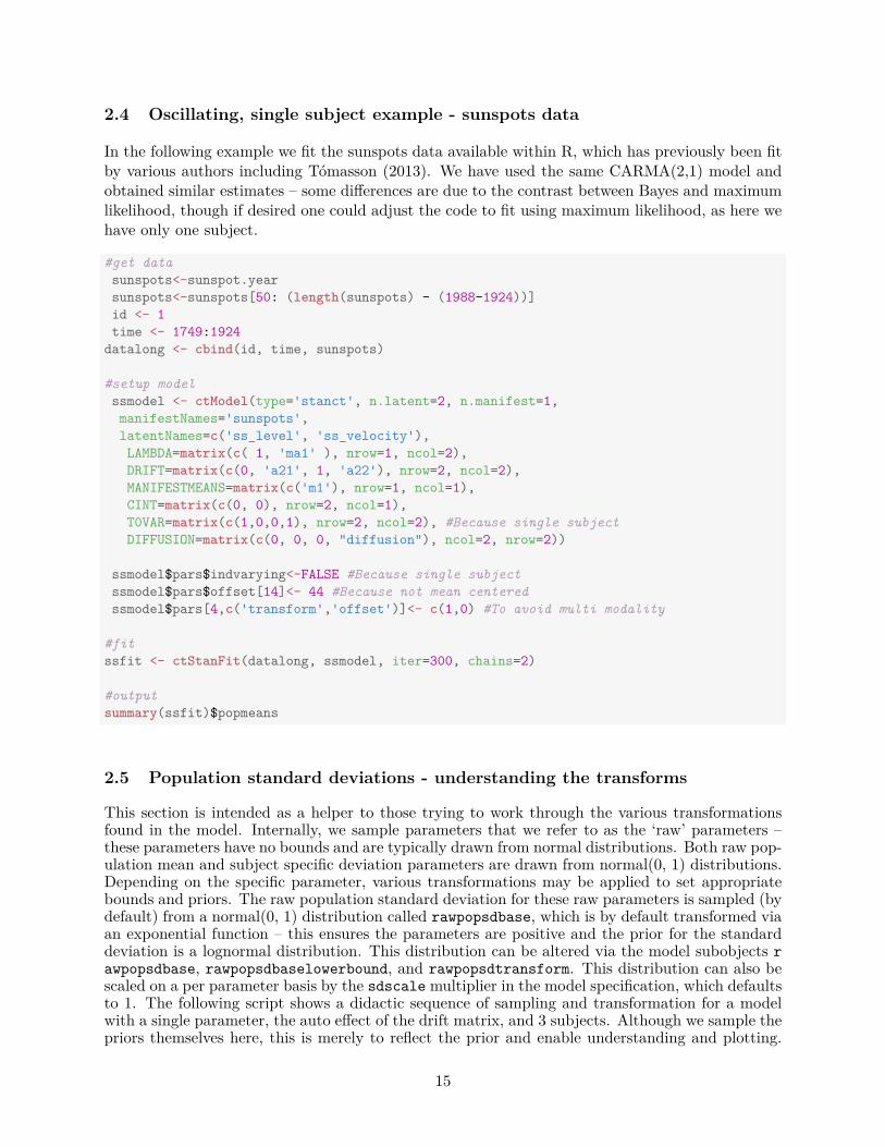
2.4 Oscillating, single subject example - sunspots data

In the following example we fit the sunspots data available within R, which has previously been fitby various authors including Tómasson (2013). We have used the same CARMA(2,1) model andobtained similar estimates – some differences are due to the contrast between Bayes and maximumlikelihood, though if desired one could adjust the code to fit using maximum likelihood, as here wehave only one subject.

#get datasunspots<-sunspot.yearsunspots<-sunspots[50: (length(sunspots) - (1988-1924))]id <- 1time <- 1749:1924

datalong <- cbind(id, time, sunspots)

#setup modelssmodel <- ctModel(type='stanct', n.latent=2, n.manifest=1,manifestNames='sunspots',latentNames=c('ss_level', 'ss_velocity'),LAMBDA=matrix(c( 1, 'ma1' ), nrow=1, ncol=2),DRIFT=matrix(c(0, 'a21', 1, 'a22'), nrow=2, ncol=2),MANIFESTMEANS=matrix(c('m1'), nrow=1, ncol=1),CINT=matrix(c(0, 0), nrow=2, ncol=1),T0VAR=matrix(c(1,0,0,1), nrow=2, ncol=2), #Because single subjectDIFFUSION=matrix(c(0, 0, 0, "diffusion"), ncol=2, nrow=2))

ssmodel$pars$indvarying<-FALSE #Because single subjectssmodel$pars$offset[14]<- 44 #Because not mean centeredssmodel$pars[4,c('transform','offset')]<- c(1,0) #To avoid multi modality

#fitssfit <- ctStanFit(datalong, ssmodel, iter=300, chains=2)

#outputsummary(ssfit)$popmeans

2.5 Population standard deviations - understanding the transforms

This section is intended as a helper to those trying to work through the various transformationsfound in the model. Internally, we sample parameters that we refer to as the ‘raw’ parameters –these parameters have no bounds and are typically drawn from normal distributions. Both raw pop-ulation mean and subject specific deviation parameters are drawn from normal(0, 1) distributions.Depending on the specific parameter, various transformations may be applied to set appropriatebounds and priors. The raw population standard deviation for these raw parameters is sampled (bydefault) from a normal(0, 1) distribution called rawpopsdbase, which is by default transformed viaan exponential function – this ensures the parameters are positive and the prior for the standarddeviation is a lognormal distribution. This distribution can be altered via the model subobjects rawpopsdbase, rawpopsdbaselowerbound, and rawpopsdtransform. This distribution can also bescaled on a per parameter basis by the sdscale multiplier in the model specification, which defaultsto 1. The following script shows a didactic sequence of sampling and transformation for a modelwith a single parameter, the auto effect of the drift matrix, and 3 subjects. Although we sample thepriors themselves here, this is merely to reflect the prior and enable understanding and plotting.

15

Note also that because we are only displaying the procedure for a single parameter here, we simplifythings somewhat by avoiding calculations to determine the square root of the population covariancematrix – with only one individually varying parameter, it is simply the standard deviation.

#set plotting parameterspar(mfrow=c(2,2), lwd=3, yaxs='i', mgp=c(1.8,.5,0),

mar=c(3,3,3,1)+.1)bw=.03

n <- 999999 #number of samples to draw to from prior for plotting purposesnsubjects <- 4 #number of subjects

#parameter specific transformtform <- function(x) -log(exp(-1.5 * x) + 1) #default drift auto effect transform

#raw pop sd transformsdscale <- 1 #defaultrawsdtform <- function(x) exp(x * 2 -2) * sdscale #default

#sd approximation functionsdapprox <- function(means,sds,tform) {

for(i in 1:length(means)){sds[i] <- ((tform(means[i]+sds[i]*3) - tform(means[i]-sds[i]*3))/6 +

(tform(means[i]+sds[i]) - tform(means[i]-sds[i]))/2) /2}return(sds)

}

#raw population mean parametersrawpopmeans_prior <- rnorm(n, 0, 1) #prior distribution for rawpopmeansrawpopmeans_sample <- -.3 #hypothetical samplesdscale <- 1 #default

#population mean parameters after parameter specific transformpopmeans_prior <- tform(rawpopmeans_prior)popmeans_sample <- tform(rawpopmeans_sample)

#plot pop meansplot(density(rawpopmeans_prior), ylim=c(0,1), xlim=c(-5,2),

xlab='Parameter value', main='Population means')points(density(popmeans_prior, bw=bw),col=2,type='l')segments(y0=0,y1=.5,x0=c(rawpopmeans_sample,popmeans_sample),lty=3,col=1:2)legend('topleft',c('Raw pop. mean prior', 'Pop. mean prior',

'Raw pop. mean sample', 'Pop. mean sample'),lty=c(1,1,3,3), col=1:2, bty='n')

#population standard deviation parametersrawpopsd_prior <- rawsdtform(rnorm(n, 0, 1)) #raw population sd prior

popsd_prior <- sdapprox(rawpopmeans_prior,rawpopsd_prior,tform)

#sample population standard deviation posteriorrawpopsd_sample <- rawsdtform(.9) #hypothetical samplepopsd_sample <- sdapprox(means=rawpopmeans_sample, #transform sample to actual pop sd

sds=rawpopsd_sample,tform=tform)

16

#plot pop sdplot(density(rawpopsd_prior,from=-.2,to=10,na.rm=TRUE, bw=bw), xlab='Parameter value',

xlim=c(-.1,3), ylim=c(0,2), main='Population sd')points(density(popsd_prior,from=-.2,to=10,na.rm=TRUE, bw=bw),type='l', col=2)segments(y0=0,y1=1,x0=c(rawpopsd_sample, popsd_sample), col=1:2,lty=3)legend('topright',c('Raw pop. sd prior','Pop. sd prior',

'Raw pop. sd sample','Pop. sd sample'), col=1:2, lty=c(1,1,3,3),bty='n')

#individual level parameters

#marginal individual level parameters (given all possible values for mean and sd)rawindparams_margprior <- rawpopmeans_prior + rawpopsd_prior * rnorm(n, 0, 1)indparams_margprior <- tform(rawindparams_margprior)

plot(density(rawindparams_margprior,from=-10,to=10,bw=bw), xlab='Parameter value',xlim=c(-5,2), ylim=c(0,1), main='Marginal dist. individual parameters')

points(density(indparams_margprior,from=-10,to=.2,bw=bw),type='l',col=2)legend('topleft',c('Raw individual parameters prior','Individual parameters prior'),

col=1:2,lty=1,bty='n')

#conditional individual level parameters (given sampled values for mean and sd)rawindparams_condprior<- rawpopmeans_sample + rawpopsd_sample * rnorm(n,0,1)rawindparams_condsample<- rawpopmeans_sample + rawpopsd_sample * rnorm(nsubjects,0,1)indparams_condprior<- tform(rawindparams_condprior)indparams_condsample<- tform(rawindparams_condsample)

plot(density(rawindparams_condprior), xlab='Parameter value', xlim=c(-5,2),ylim=c(0,1), main='Conditional dist. individual parameters')

points(density(indparams_condprior),type='l',col=2)segments(y0=0,y1=.5,x0=c(rawindparams_condsample, indparams_condsample),

col=rep(1:2,each=nsubjects),lty=3, lwd=2)legend('topleft',c('Raw ind. pars. prior','Ind. pars. prior',

'Raw ind. pars. samples','Ind. pars. samples'), col=1:2, lty=c(1,1,3,3),bty='n')

In the top left of Figure 7, we can see the prior distribution of population means for, in this case,a diagonal (auto effect) of the drift matrix. The prior for the raw population distribution is astandard normal, while for the actual population distribution it is definitely not normal. We drawa hypothetical sample from the raw distribution, and show the resulting transformed value. To theright, the prior distribution of the raw population standard deviation is shown. This raw distribu-tion is the same for all parameter types, but the resulting prior distribution of population standanddeviations is also dependent on the parameter specific transform (although in this particular casethe raw and actual population sd priors are almost the same). This dependency is most easilyunderstood if one considers the case where the parameter specific transformation simply multipliedthe raw parameter by 2 – if we sampled a raw population sd of 1.5, the actual population sd samplewould be 3.0. With nonlinear transformations, the dependency is not so easily calculated, andwe use a sigma point approximation (Julier & Uhlmann, 1997), as shown in the code, when it isnecessary to plot or summarise the population sd. The lower left plot shows the prior distributionfor individual level parameters, marginalising over the priors for population means and standarddeviations. This plot is very similar to the means plot directly above it, just somewhat more spread

17

−5 −4 −3 −2 −1 0 1 2

0.0

0.2

0.4

0.6

0.8

1.0

Population means

Parameter value

Den

sity

Raw pop. mean priorPop. mean priorRaw pop. mean samplePop. mean sample

0.0 0.5 1.0 1.5 2.0 2.5 3.0

0.0

0.5

1.0

1.5

2.0

Population sd

Parameter value

Den

sity

Raw pop. sd priorPop. sd priorRaw pop. sd samplePop. sd sample

−5 −4 −3 −2 −1 0 1 2

0.0

0.2

0.4

0.6

0.8

1.0

Marginal dist. individual parameters

Parameter value

Den

sity

Raw individual parameters priorIndividual parameters prior

−5 −4 −3 −2 −1 0 1 2

0.0

0.2

0.4

0.6

0.8

1.0

Conditional dist. individual parameters

Parameter value

Den

sity

Raw ind. pars. priorInd. pars. priorRaw ind. pars. samplesInd. pars. samples

Figure 7: Depiction of the prior distributions and sampling process through which individualspecific parameters are determined.

18

out due to the additional variation included. Things get more interesting when we look at the lowerright plot – here, we see the prior distributions for individual level parameters, conditional on thevalues sampled in the top row of plots. Along with the prior distribution, in this lower right plot wealso draw samples for 4 subjects, showing both the raw individual parameter, and the individualparameter after the necessary transforms.

3 Conclusion

With this work, we have described the basics of the hierarchical continuous time dynamic model,and provided detailed discussion on the usage of the R package ctsem (Driver et al., 2017) forfitting such models to data. While the model is necessarily somewhat complex, we believe it offersmany interesting possibilities for understanding the dynamics of personality over time, and hopethat the overview of the software provided here encourages new and interesting applications of themodel.

References

Driver, C. C., Oud, J. H. L. & Voelkle, M. C. (2017). Continuous time structural equation modelingwith r package ctsem. Journal of Statistical Software, 77 (5). doi:10.18637/jss.v077.i05

Driver, C. C. & Voelkle, M. C. (in press). Hierarchical Bayesian continuous time dynamic modeling.Psychological Methods.

Driver, C. C. & Voelkle, M. C. (2017). Understanding the time course of interventions with con-tinuous time dynamic models. Manuscript submitted for publication.

Gelman, A., Carlin, J. B., Stern, H. S. & Rubin, D. B. (2014). Bayesian data analysis. Chapman &Hall/CRC Boca Raton, FL, USA. Retrieved from http://amstat.tandfonline.com/doi/full/10.1080/01621459.2014.963405

Julier, S. J. & Uhlmann, J. K. (1997). New extension of the Kalman filter to nonlinear systems.(Vol. 3068, pp. 182–194). Signal Processing, Sensor Fusion, and Target Recognition VI. In-ternational Society for Optics and Photonics. doi:10.1117/12.280797

Oud, J. H. L. & Jansen, R. A. R. G. (2000). Continuous time state space modeling of panel databy means of SEM. Psychometrika, 65 (2), 199–215. doi:10.1007/BF02294374

R Core Team. (2014). R: A language and environment for statistical computing. Vienna, Austria:R Foundation for Statistical Computing. Retrieved from http://www.R-project.org/

Singer, H. (1993). Continuous-time dynamical systems with sampled data, errors of measurementand unobserved components. Journal of Time Series Analysis, 14 (5), 527–545. 00046. doi:10.1111/j.1467-9892.1993.tb00162.x

Tómasson, H. (2013). Some computational aspects of Gaussian CARMA modelling. Statistics andComputing, 25 (2), 375–387. doi:10.1007/s11222-013-9438-9

Voelkle, M. C. & Oud, J. H. L. (2013). Continuous time modelling with individually varying timeintervals for oscillating and non-oscillating processes. British Journal of Mathematical andStatistical Psychology, 66 (1), 103–126. doi:10.1111/j.2044-8317.2012.02043.x

19