Labor Economics, Pardee RAND Graduate School, Winter 2009, Page 1

1 Evans and Jovanovic (1989) Model of En-

trepreneurial Credit Constraints

Individuals can choose to be entrepreneurs or work as wage workers. Wageworkers receive w for working. Entrepreneurial income depends on entrepreneurialskill θ and earnings (y) are produced according to the production function:

y = θkα

where k represents the amount of capital invested in the venture and 0 < α < 1is a technology parameter. Entrepreneurial income is given by:

I = y + r(z − k)

where z is initial wealth and r is the interest rate. We suppose credit con-straints on the entrepreneur such that k ≤ λz, where λ ≥ 1 is the measure ofconstraints. The entrepreneur can be a new saver or a net borrower dependingon whether k∗ > z.

To analyze the choice of whether to become an entrepreneur, first considerthe choice of k for the entrepreneur:

maxk

θkα + r(z − k)

F.O.C αθkα−1 − r = 0

For an interior solution:

k∗ =

(αθ

r

) 11−α

= bθ1

1−α

where b =(αr

) 11−α . The entrepreneur will be unconstrained whenever the

optimal k∗ is below λz, i.e.

θ ≤ r

α(λz)1−α (1)

To determine whether or not to become an entrepreneur, the individual com-pares earnings under entrepreneurship to wage earnings (in both cases shereceives interest income on her wealth, so this terms drops out of the calcula-tion), i.e.:

I = max{

(bα − rb)θ1

1−α , w}

if θ ≤ r

α(λz)1−α (2)

= max {θ(λz)α − rλz, w} if θ >r

α(λz)1−α (3)

1

Labor Economics, Pardee RAND Graduate School, Winter 2009, Page 2

A little algebra can show that bα − rb is unambiguously positive. Notice thatin the unconstrained situation whether or not the person chooses to becomean entrepreneur depends solely on the value of θ, not on initial wealth. Theywill become an entrepreneur whenever θ exceeds a cutoff value.

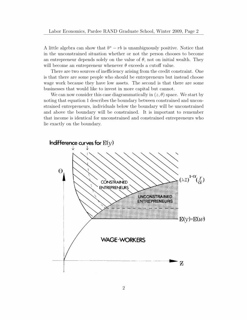
There are two sources of inefficiency arising from the credit constraint. Oneis that there are some people who should be entrepreneurs but instead choosewage work because they have low assets. The second is that there are somebusinesses that would like to invest in more capital but cannot.

We can now consider this case diagrammatically in (z, θ) space. We start bynoting that equation 1 describes the boundary between constrained and uncon-strained entrepreneurs, individuals below the boundary will be unconstrainedand above the boundary will be constrained. It is important to rememberthat income is identical for unconstrained and constrained entrepreneurs wholie exactly on the boundary.

2

Labor Economics, Pardee RAND Graduate School, Winter 2009, Page 3

In the unconstrained region, as explained above there is some cutoff valueof θ above which people become entrepreneurs, and this does not depend ontheir level of z. In this region capital invested is the same for all agents and soare the returns from being an entrepreneur (since these returns are determinedonly by the amount of capital).

To see the shape of the indifference curves in the constrained region, wecan set (3) equal to some sort of constant I and then solve for θ in terms of z,which yields θ = I(λz)−α + r(λz)1−α.

Suppose that z and θ are uncorrelated. Several empirical predictions arisefrom this model:

1. The probability of starting a business is correlated with initial wealthonly when there are credit constraints. This follows from the fact thatin the unconstrained case z does not enter into the final maximization.

2. Wealthier entrepreneurs will enjoy higher levels of entrepreneurial re-turns, because they have more capital to invest. We can see this bynoting that as z increases, we are able to hit higher level curves on theindifference map.

3. Poorer entrepreneurs must devote a larger proportion of their assets totheir businesses.

4. Smaller firms will grow faster than larger firms started at the same time.This occurs because smaller firms will be initially credit constrained andwill thus have more incentive to invest profits back into the business,generating growth. To see this, think about a person who starts in theconstrained region of the chart. θ remains constant over time, but overtime z increases. At some point the individual will shift from the con-strained to the unconstrained zone. Notice that once someone is in theunconstrained zone, further increases in z no longer increase investmentin the business; this follows from point (1).

5. Over time, assets should become a less important determinant of firmreturns because smaller firms will be able to overcome the credit con-straint and catch up with larger firms. This follows from the same logicas point (4)–essentially at some point all the small firms will move intothe unconstrained zone, and then investment and returns are fixed goingforward.

Are there any potential policy implications of the model? Think about a policythat provided better education, which increased people’s level of θ. One thing

3

Labor Economics, Pardee RAND Graduate School, Winter 2009, Page 4

that we can see is that if individuals are sufficiently poor (low z), such apolicy will not actually increase entrepreneurship. Diagrammatically this islike moving up and down in the region to the left of the indifference curves.This might be a reasonable description of some developing countries.

Alternatively, we can think of a policy that offers subsidies for individualsstarting small businesses. This model predicts that such subsidies would bevaluable only to more skilled entrepreneurs. Many subsidies to entrepreneursare targeted towards certain types of individuals (e.g., minority set-asides, mi-crocredit loans to poor/women, entrepreneur competitions for MBA students).If these characteristics are correlated with entrepreneurial ability, that couldincrease or decrease the efficacy of such subsidy programs.

Reference

Evans, David S. and Boyan Jovanovic. 1989. “An Estimated Model of En-trepreneurial Choice under Liquidity Constraints.” Journal of Political Econ-omy 97(4) 808-827.

4