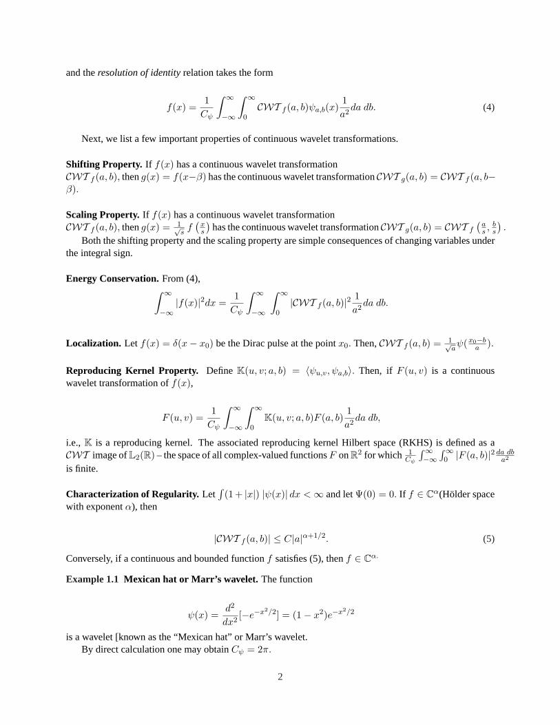
ISyE8843A, Brani Vidakovic Handout 20

1 Basics of Wavelets

The first theoretical results in wavelets are connected with continuous wavelet decompositions ofL2 func-tions and go back to the early 1980s. Papers of Morletet al. (1982) and Grossmann and Morlet (1985) wereamong the first on this subject.

Let ψa,b(x), a ∈ R\{0}, b ∈ R be a family of functions defined as translations and re-scales of a singlefunctionψ(x) ∈ L2(R),

ψa,b(x) =1√|a|ψ

(x− b

a

). (1)

Normalization by 1√|a| ensures that||ψa,b(x)|| is independent ofa andb. The functionψ (called the

wavelet functionor the mother wavelet) is assumed to satisfy theadmissibility condition,

Cψ =∫

R

|Ψ(ω)|2|ω| dω < ∞, (2)

whereΨ(ω) =∫R ψ(x)e−ixωdx is the Fourier transformation ofψ(x). The admissibility condition (2)

implies

0 = Ψ(0) =∫

ψ(x)dx.

Also, if∫

ψ(x)dx = 0 and∫

(1 + |x|α)|ψ(x)|dx < ∞ for someα > 0, thenCψ < ∞.Wavelet functions are usually normalized to “have unit energy”, i.e.,||ψa,b(x)|| = 1.For anyL2 functionf(x), the continuous wavelet transformation is defined as a function of two variables

CWT f (a, b) = 〈f, ψa,b〉 =∫

f(x)ψa,b(x)dx.

Here the dilation and translation parameters,a andb, respectively, vary continuously overR\{0} × R.

Resolution of Identity. When the admissibility condition is satisfied, i.e.,Cψ < ∞, it is possible to find theinverse continuous transformation via the relation known asresolution of identityor Calderon’s reproducingidentity,

f(x) =1

Cψ

∫

R2

CWT f (a, b)ψa,b(x)da db

a2.

If a is restricted toR+, which is natural sincea can be interpreted as a reciprocal of frequency, (2)becomes

Cψ =∫ ∞

0

|Ψ(ω)|2ω

dω < ∞, (3)

1

and theresolution of identityrelation takes the form

f(x) =1

Cψ

∫ ∞

−∞

∫ ∞

0CWT f (a, b)ψa,b(x)

1a2

da db. (4)

Next, we list a few important properties of continuous wavelet transformations.

Shifting Property. If f(x) has a continuous wavelet transformationCWT f (a, b), theng(x) = f(x−β) has the continuous wavelet transformationCWT g(a, b) = CWT f (a, b−β).

Scaling Property. If f(x) has a continuous wavelet transformationCWT f (a, b), theng(x) = 1√

sf

(xs

)has the continuous wavelet transformationCWT g(a, b) = CWT f

(as , b

s

).

Both the shifting property and the scaling property are simple consequences of changing variables underthe integral sign.

Energy Conservation.From (4),∫ ∞

−∞|f(x)|2dx =

1Cψ

∫ ∞

−∞

∫ ∞

0|CWT f (a, b)|2 1

a2da db.

Localization. Let f(x) = δ(x− x0) be the Dirac pulse at the pointx0. Then,CWT f (a, b) = 1√aψ(x0−b

a ).

Reproducing Kernel Property. DefineK(u, v; a, b) = 〈ψu,v, ψa,b〉. Then, if F (u, v) is a continuouswavelet transformation off(x),

F (u, v) =1

Cψ

∫ ∞

−∞

∫ ∞

0K(u, v; a, b)F (a, b)

1a2

da db,

i.e.,K is a reproducing kernel. The associated reproducing kernel Hilbert space (RKHS) is defined as aCWT image ofL2(R) – the space of all complex-valued functionsF onR2 for which 1

Cψ

∫∞−∞

∫∞0 |F (a, b)|2 da db

a2

is finite.

Characterization of Regularity. Let∫

(1 + |x|) |ψ(x)| dx < ∞ and letΨ(0) = 0. If f ∈ Cα(Holder spacewith exponentα), then

|CWT f (a, b)| ≤ C|a|α+1/2. (5)

Conversely, if a continuous and bounded functionf satisfies (5), thenf ∈ Cα.

Example 1.1 Mexican hat or Marr’s wavelet. The function

ψ(x) =d2

dx2[−e−x2/2] = (1− x2)e−x2/2

is a wavelet [known as the “Mexican hat” or Marr’s wavelet.By direct calculation one may obtainCψ = 2π.

2

rrr rrrrr r r rr r r r r r rrrrrrr

r r r r r r r r r r r r rrrrrrrrrrrrr

r r r r r r r r r r r r r r r r rr r r r r r r r rrrrrrrrrrrrrrrrrrrrrrrrrr

-b0

6a

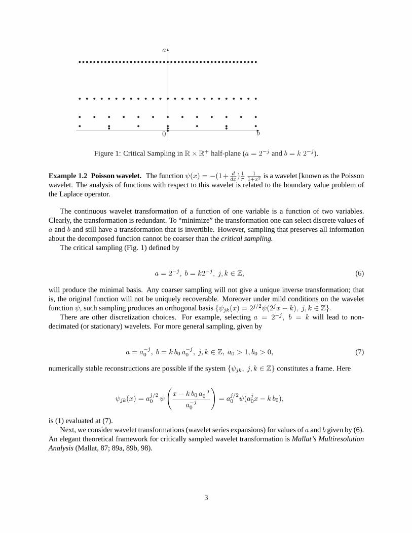
Figure 1: Critical Sampling inR× R+ half-plane (a = 2−j andb = k 2−j).

Example 1.2 Poisson wavelet.The functionψ(x) = −(1+ ddx) 1

π1

1+x2 is a wavelet [known as the Poissonwavelet. The analysis of functions with respect to this wavelet is related to the boundary value problem ofthe Laplace operator.

The continuous wavelet transformation of a function of one variable is a function of two variables.Clearly, the transformation is redundant. To “minimize” the transformation one can select discrete values ofa andb and still have a transformation that is invertible. However, sampling that preserves all informationabout the decomposed function cannot be coarser than thecritical sampling.

The critical sampling (Fig. 1) defined by

a = 2−j , b = k2−j , j, k ∈ Z, (6)

will produce the minimal basis. Any coarser sampling will not give a unique inverse transformation; thatis, the original function will not be uniquely recoverable. Moreover under mild conditions on the waveletfunctionψ, such sampling produces an orthogonal basis{ψjk(x) = 2j/2ψ(2jx− k), j, k ∈ Z}.

There are other discretization choices. For example, selectinga = 2−j , b = k will lead to non-decimated (or stationary) wavelets. For more general sampling, given by

a = a−j0 , b = k b0 a−j

0 , j, k ∈ Z, a0 > 1, b0 > 0, (7)

numerically stable reconstructions are possible if the system{ψjk, j, k ∈ Z} constitutes a frame. Here

ψjk(x) = aj/20 ψ

(x− k b0 a−j

0

a−j0

)= a

j/20 ψ(aj

0x− k b0),

is (1) evaluated at (7).Next, we consider wavelet transformations (wavelet series expansions) for values ofa andb given by (6).

An elegant theoretical framework for critically sampled wavelet transformation isMallat’s MultiresolutionAnalysis(Mallat, 87; 89a, 89b, 98).

3

1.1 Multiresolution Analysis

A multiresolution analysis (MRA) is a sequence of closed subspacesVn, n ∈ Z in L2(R) such that they liein a containment hierarchy

· · · ⊂ V−2 ⊂ V−1 ⊂ V0 ⊂ V1 ⊂ V2 ⊂ · · · . (8)

The nested spaces have an intersection that contains the zero function only and a union that is dense inL(R),

∩nVj = {0}, ∪jVj = L2(R).

[With A we denoted the closure of a setA]. The hierarchy (8) is constructed such that (i)V -spaces areself-similar,

f(2jx) ∈ Vj iff f(x) ∈ V0. (9)

and (ii) there existsa scaling functionφ ∈ V0 whose integer-translates span the spaceV0,

V0 =

{f ∈ L2(R)| f(x) =

∑

k

ckφ(x− k)

},

and for which the set{φ(• − k), k ∈ Z} is an orthonormal basis.1

Mild technical conditions onφ are necessary for future developments. It can be assumed that∫

φ(x)dx ≥0. Later, we will prove that this integral is in fact equal to 1. SinceV0 ⊂ V1, the functionφ(x) ∈ V0 can berepresented as a linear combination of functions fromV1, i.e.,

φ(x) =∑

k∈Zhk

√2φ(2x− k), (10)

for some coefficientshk, k ∈ Z. This equation is called thescaling equation(or two-scale equation) and itis fundamental in constructing, exploring, and utilizing wavelets.

ADD BASES FORVj .ANY L2 can be projected onVj

In the wavelet literature, the reader may encounter an indexing of the multiresolution subspaces, whichis the reverse of that in (8),

· · · ⊂ V2 ⊂ V1 ⊂ V0 ⊂ V−1 ⊂ V−2 ⊂ · · · . (11)

FORM OFφjk(x).

1It is possible to relax the orthogonality requirement. It is sufficient to assume that the system of functions{φ(• − k), k ∈ Z}constitutes a Riesz basis forV0.

4

Theorem 1.1 For the scaling function it holds∫

Rφ(x)dx = 1,

or, equivalently,Φ(0) = 1,

whereΦ(ω) is Fourier transformation ofφ,∫R φ(x)e−iωxdx.

The coefficientshn in (10) are important in connecting the MRA to the theory of signal processing. The(possibly infinite) vectorh = {hn, n ∈ Z} will be called awavelet filter.It is a low-pass (averaging) filteras will become clear later by considerations in the Fourier domain.

To further explore properties of multiresolution analysis subspaces and their bases, we will often workin the Fourier domain. Define the functionm0 as follows:

m0(ω) =1√2

∑

k∈Zhke

−ikω =1√2H(ω). (12)

The function in (12) is sometimes called thetransfer functionand it describes the behavior of the associatedfilter h in the Fourier domain. Notice that the functionm0 is periodic with the period2π and that the filtertaps{hn, n ∈ Z} are the Fourier coefficients of the functionH(ω) =

√2 m0(ω).

In the Fourier domain, the relation (10) becomes

Φ(ω) = m0

(ω

2

)Φ

(ω

2

), (13)

whereΦ(ω) is the Fourier transformation ofφ(x). Indeed,

Φ(ω) =∫ ∞

−∞φ(x)e−iωxdx

=∑

k

√2 hk

∫ ∞

−∞φ(2x− k)e−iωxdx

=∑

k

hk√2e−ikω/2

∫ ∞

−∞φ(2x− k)e−i(2x−k)ω/2d(2x− k)

=∑

k

hk√2e−ikω/2 Φ

(ω

2

)

= m0

(ω

2

)Φ

(ω

2

).

By iterating (13), one gets

Φ(ω) =∞∏

n=1

m0

( ω

2n

), (14)

which is convergent under very mild conditions on rates of decay of the scaling functionφ. There areseveral sufficient conditions for convergence of the product in (14). For instance, the uniform convergence

5

on compact sets is assured if (i)m0(ω) = 1 and (ii) |m0(ω) − 1| < C|ω|ε, for some positiveC andε. Seealso Theorem 1.2.

Next, we prove two important properties of wavelet filters associated with an orthogonal multiresolutionanalysis,normalizationandorthogonality.

Normalization.

∑

k∈Zhk =

√2. (15)

Proof:

∫φ(x)dx =

√2

∑

k

hk

∫φ(2x− k)dx

=√

2∑

k

hk12

∫φ(2x− k)d(2x− k)

=√

22

∑

k

hk

∫φ(x)dx.

Since∫

φ(x)dx 6= 0 by assumption, (15) follows.

This result also follows fromm0(0) = 1.

Orthogonality. For anyl ∈ Z,

∑

k

hkhk−2l = δl. (16)

Proof: Notice first that from the scaling equation (10) it follows that

φ(x)φ(x− l) =√

2∑

k

hkφ(2x− k)φ(x− l) (17)

=√

2∑

k

hkφ(2x− k)√

2∑m

hmφ(2(x− l)−m).

By integrating the both sides in (17) we obtain

δl = 2∑

k

hk

[∑m

hm12

∫φ(2x− k)φ(2x− 2l −m) d(2x)

]

=∑

k

∑m

hkhmδk,2l+m

=∑

k

hkhk−2l.

The last line is obtained by takingk = 2l + m.

6

An important special case isl = 0 for which (16) becomes

∑

k

h2k = 1. (18)

One consequence of the orthogonality condition (16) is the following: the convolution of filterh withitself, f = h ? h, is ana trous.2

The fact that the system{φ(• − k), k ∈ Z} constitutes an orthonormal basis forV0 can be expressed inthe Fourier domain in terms of eitherΦ(ω) or m0(ω).

(a) In terms ofΦ(ω):

∞∑

l=−∞|Φ(ω + 2πl)|2 = 1. (19)

By the[PAR] property of the Fourier transformation and the2π-periodicity ofeiωk one has

δk =∫

Rφ(x)φ(x− k)dx

=12π

∫

RΦ(ω)Φ(ω)eiωkdω

=12π

∫ 2π

0

∞∑

l=−∞|Φ(ω + 2πl)|2eiωkdω. (20)

The last line in (20) is the Fourier coefficientak in the Fourier series decomposition of

f(ω) =∞∑

l=−∞|Φ(ω + 2πl)|2.

Due to the uniqueness of Fourier representation,f(ω) = 1. As a side results, we obtain thatΦ(2πn) =0, n 6= 0, and

∑n φ(x − n) = 1. The last result follows from inspection of coefficientsck in the Fourier

decomposition of∑

n φ(x− n), the series∑

k cke2πikx. Since this function is 1-periodic,

ck =∫ 1

0

(∑n

φ(x− n)

)e−2πikxdx =

∫ ∞

−∞φ(x)e−2πikxdx = Φ(2πk) = δ0,k.

Remark 1.1 Utilizing the identity (19), any set of independent functions spanningV0, {φ(x− k), k ∈ Z},can be orthogonalized in the Fourier domain. The orthonormal basis is generated by integer-shifts of thefunction

F−1

Φ(ω)√∑∞

l=−∞ |Φ(ω + 2πl)|2

. (21)

This normalization in the Fourier domain is used in constructing of some wavelet bases.

2The attributea trous (Fr.) ( ≡ with holes) comes from the propertyf2n = δn, i.e., each tap on even position inf is 0, exceptthe tapf0. Such filters are also called half-band filters.

7

(b) In terms ofm0 :

|m0(ω)|2 + |m0(ω + π)|2 = 1. (22)

Since∑∞

l=−∞ |Φ(2ω + 2lπ)|2 = 1, then by (13)

∞∑

l=−∞|m0(ω + lπ)|2|Φ(ω + lπ)|2 = 1. (23)

Now split the sum in (23) into two sums – one with odd and the other with even indices, i.e.,

1 =∞∑

k=−∞|m0(ω + 2kπ)|2|Φ(ω + 2kπ)|2 +

∞∑

k=−∞|m0(ω + (2k + 1)π)|2|Φ(ω + (2k + 1)π)|2.

To simplify the above expression, we use relation (19) and the2π-periodicity ofm0(ω).

1 = |m0(ω)|2∞∑

k=−∞|Φ(ω + 2kπ)|2 + |m0(ω + π)|2

∞∑

k=−∞|Φ((ω + π) + 2kπ)|2

= |m0(ω)|2 + |m0(ω + π)|2.

Whenever a sequence of subspaces satisfies MRA properties, there exists (though not unique) an or-thonormal basis forL2(R),

{ψjk(x) = 2j/2ψ(2jx− k), j, k ∈ Z} (24)

such that{ψjk(x), j-fixed, k ∈ Z} is an orthonormal basis of the “difference space”Wj = Vj+1ªVj . Thefunctionψ(x) = ψ00(x) is called awavelet functionor informally the mother wavelet.

Next, we detail the derivation of a wavelet function from the scaling function. Sinceψ(x) ∈ V1 (becauseof the containmentW0 ⊂ V1), it can be represented as

ψ(x) =∑

k∈Zgk

√2φ(2x− k), (25)

for some coefficientsgk, k ∈ Z.Define

m1(ω) =1√2

∑

k

gke−ikω. (26)

8

By mimicking what was done withm0, we obtain the Fourier counterpart of (25),

Ψ(ω) = m1(ω

2)Φ(

ω

2). (27)

The spacesW0 andV0 are orthogonal by construction. Therefore,

0 =∫

ψ(x)φ(x− k)dx =12π

∫Ψ(ω)Φ(ω)eiωkdω

=12π

∫ 2π

0

∞∑

l=−∞Ψ(ω + 2lπ)Φ(ω + 2lπ)eiωkdω.

By repeating the Fourier series argument, as in (19), we conclude

∞∑

l=−∞Ψ(ω + 2lπ)Φ(ω + 2lπ) = 0.

By taking into account the definitions ofm0 andm1, and by mimicking the derivation of (22), we find

m1(ω)m0(ω) + m1(ω + π)m0(ω + π) = 0. (28)

From (28), we conclude that there exists a functionλ(ω) such that

(m1(ω), m1(ω + π) ) = λ(ω)(m0(ω + π), −m0(ω)

). (29)

By substitutingξ = ω + π and by using the2π-periodicity ofm0 andm1, we conclude that

λ(ω) = −λ(ω + π), and (30)

λ(ω) is 2π-periodic.

Any function λ(ω) of the forme±iωS(2ω), whereS is anL2([0, 2π]), 2π-periodic function, will satisfy(28); however, only the functions for which|λ(ω)| = 1 will define an orthogonal basisψjk of L2(R).

To summarize, we chooseλ(ω) such that

(i) λ(ω) is 2π-periodic,

(ii) λ(ω) = −λ(ω + π), and

(iii) |λ(ω)|2 = 1.

Standard choices forλ(ω) are−e−iω, e−iω, andeiω; however, any other function satisfying (i)-(iii) willgenerate a validm1. We choose to definem1(ω) as

m1(ω) = −e−iωm0(ω + π). (31)

9

since it leads to a convenient and standard connection between the filtersh andg.The form ofm1 and the equation (19) imply that{ψ(• − k), k ∈ Z} is an orthonormal basis forW0.Since|m1(ω)| = |m0(ω + π)|, the orthogonality condition (22) can be rewritten as

|m0(ω)|2 + |m1(ω)|2 = 1. (32)

By comparing the definition ofm1 in (26) with

m1(ω) = −e−iω 1√2

∑

k

hkei(ω+π)k

=1√2

∑

k

(−1)1−khke−iω(1−k)

=1√2

∑n

(−1)nh1−ne−iωn,

we relategn andhn as

gn = (−1)n h1−n. (33)

In signal processing literature, the relation (33) is known as thequadrature mirror relationand the filtershandg asquadrature mirror filters.

Remark 1.2 Choosingλ(ω) = eiω leads to the rarely used high-pass filtergn = (−1)n−1 h−1−n. It issometimes convenient to definegn as(−1)nh1−n+M , whereM is a “shift constant.” Such re-indexing ofgaffects only the shift-location of the wavelet function.

1.2 Haar Wavelets

In addition to their simplicity and formidable applicability, Haar wavelets have tremendous educationalvalue. Here we illustrate some of the relations discussed in the Section 1.1 using the Haar wavelet. We startwith φ(x) = 1(0 ≤ x ≤ 1) and pretend that everything else is unknown.

The scaling equation (10) is very simple for the Haar case. By inspection of simple graphs of two scaledHaar waveletsφ(2x) andφ(2x + 1) stuck to each other, we conclude that the scaling equation is

φ(x) = φ(2x) + φ(2x− 1)

=1√2

√2φ(2x) +

1√2

√2φ(2x− 1), (34)

which yields the wavelet filter coefficients:

h0 = h1 =1√2.

Now, the transfer functions become

10

m0(ω) =1√2

(1√2e−iω0

)+

1√2

(1√2e−iω1

)=

1 + e−iω

2.

and

m1(ω) = −e−iω m0(ω + π) = −e−iω

(12− 1

2eiω

)=

1− e−iω

2.

Notice thatm0(ω) = |m0(ω)|eiϕ(ω) = cos ω2 · e−iω/2 (aftercosx = eix+e−ix

2 ). Sinceϕ(ω) = −ω2 , Haar’s

wavelet haslinear phase,i.e., the scaling function is symmetric in the time domain. The orthogonalitycondition|m0(ω)|2 + |m1(ω)|2 = 1 is easily verified, as well.

Relation (27) becomes

Ψ(ω) =1− e−iω/2

2Φ

(ω

2

)=

12Φ

(ω

2

)− 1

2Φ

(ω

2

)e−iω/2,

and by applying the inverse Fourier transformation we obtain

ψ(x) = φ(2x)− φ(2x− 1)

in the time-domain. Therefore we “discovered” the Haar wavelet functionψ. From the expression form1

or by inspecting the representation ofψ(x) by φ(2x) andφ(2x− 1), we “conclude” thatg0 = −g−1 = 1√2.

The Haar basis is not an appropriate basis for all applications for several reasons. The building blocks inHaar’s decomposition are discontinuous functions that obviously are not effective in approximating smoothfunctions. Although the Haar wavelets are well localized in the time domain, in the frequency domain theydecay at the slow rate ofO( 1

n).

1.3 Daubechies’ Compactly Supported Wavelets

Daubechies was first to construct compactly supported orthogonal wavelets with a preassigned degree ofsmoothness. Here we present the idea of Daubechies, omitting some technical details. Detailed treatment ofthis topic can be found in the monograph Daubechies (1992), Chapters 6 and 7.

Suppose thatψ hasN (≥ 2) vanishing moments, i.e.,∫

xnψ(x)dx = 0, n = 0, 1, . . . , N − 1. Them0(ω) has the form:

m0(ω) =(

1 + e−iω

2

)N

L(ω), (35)

whereL(ω) is a trigonometric polynomial. Indeed, sinceψ hasN vanishing moments, thenΨ(n)(0) =0, n = 0, 1, . . . , N − 1. By differentiating (27), we get

[m1(ω)Φ(ω)](n)ω=0 = 0, n = 0, 1, . . . , N − 1.

SinceΦ(0) = 1, it follows thatm(n)1 (0) or, equivalently,m(n)

0 (π) = 0, for n = 0, 1, . . . , N − 1. Thus,m0(ω) has to be as in (35).

11

In terms of

M0(ω) = |m0(ω)|2 =(cos2

ω

2

)N· |L(ω)|2,

the orthogonality condition (22) becomes

M0(ω) + M0(ω + π) = 1. (36)

|L(ω)|2 is a polynomial incosω. It can be re-expressed as a polynomial iny = sin2 ω2 sincecosω =

1−2 sin2 ω2 . This re-expression is beneficial since we can use some standard results in theory of polynomials,

to specify|L(ω)|2. Denote this polynomial byP (sin2 ω2 ). In terms of the polynomialP the orthogonality

condition (36) becomes

(1− y)NP (y) + yNP (1− y) = 1, (y = sin2 ω

2). (37)

By Bezout’s result (outlined below), there exists a unique solution of the functional equation (37). It canbe found by the Euclidean algorithm since the polynomials(1− y)N andyN are relatively prime.

Lemma 1.1 (Bezout) Ifp1 andp2 are two polynomials of degreen1 andn2, respectively, with no commonzeroes, then there exist unique polynomialsq1 andq2 of degreen2 − 1 andn1 − 1, respectively, so that

p1(x)q1(x) + p2(x)q2(x) = 1.

For the proof of the lemma, we direct the reader to Daubechies ([?], 169-170). The unique solution of (37)with degreedeg(P (y)) ≤ N − 1 is

N−1∑

k=0

(N + k − 1

k

)yk, y = sin2 ω

2, (38)

and since it is positive fory ∈ [0, 1], it does not contradict the positivity of|L(ω)|2.Remark: If the degree of a solution is not required to be minimal then any other polynomialQ(y) =P (y) + yNR(1

2 − y) whereR is an odd polynomial preserving the positivity ofQ, will lead to a differentsolution form0(ω). By choosingR 6= 0, one can generalize the standard Daubechies family, to constructsymmlets, complex Daubechies wavelets, coiflets, etc.

The function|m0(ω)|2 is now completely determined. To finish the construction we have to find itssquare root. A result of Riesz, known as thespectral factorization lemma, makes this possible.

Lemma 1.2 (Riesz) LetA be a positive trigonometric polynomial with the propertyA(−x) = A(x). Then,A is necessarily of the form

A(x) =M∑

m=1

um cosmx.

In addition, there exists a polynomialB of the same orderB(x) =∑M

m=1 vmeimx such that|B(x)|2 =A(x). If the coefficientsum are real, thenB can be chosen so that the coefficientsvm are also real.

12

We first represent|L(ω)|2 as the polynomial

a0

2+

N−1∑

k=1

ak cosk ω,

by replacingsin2 ω2 in (38) by 1−cos ω

2 .An auxiliary polynomialPA, such that|L(e−iω)|2 = |PA(e−iω)|, is formed.If z = e−iω, thencosω = z+z−1

2 and one such auxiliary polynomial is

PA(z) =12

N−1∑

k=1−N

a|k|zN−1+k. (39)

SincePA(z) = z2N−2PA(1z ), the zeroes ofPA(z) appear in reciprocal pairs if real, and quadruples(zi, zi, z

−1i , z−1

i )if complex. Without loss of generality we assume thatzj , zj andrj lie outside the unit circle in the complexplane. Of course, thenz−1

j , z−1j andr−1

j lie inside the unit circle. The factorized polynomialPA can bewritten as

PA(z) =12aN−1

[I∏

i=1

(z − ri)(z − 1ri

)

]

J∏

j=1

(z − zj)(z − zj)(z − z−1j )(z − z−1

j )

. (40)

Herer1, r2, . . . , rI are real and non zero, andz1, . . . , zJ are complex;I + 2J = N − 1.The goal is to take a square root from|PA(z)| and the following simple substitution puts|PA(z)| in a

convenient form.Sincez = e−iω, we replace|(z − zj)(z − z−1

j )| by |zj |−1|z − zj |2, and the polynomial|PA| becomes

12|aN−1|

I∏

i=1

|r−1i |

J∏

j=1

|zj |−2 · |I∏

i=1

(z − ri)J∏

j=1

(z − zj)(z − zj)|2.

Now,L(ω) becomes

±(12|aN−1|

I∏

i=1

|r−1i |

J∏

j=1

|zj |−2)12

· |I∏

i=1

(z − ri)J∏

j=1

(z − zj)(z − zj)|, z = e−iω, (41)

where the sign is chosen so thatm0(0) = L(0) = 1. Note thatdeg[PA(z)] = deg[|L(z)|2] = N − 1.Finally, the coefficientsh0, h1, . . . , h2N−1 in the polynomial

√2 m0(ω) are the desired wavelet filter

coefficients.

13

Example 1.3 We will find m0 for N = 2.|L(ω)|2 =

∑2−1k=0

(2+k−1

k

)sin2 kω

2 = 1 + 21−cos ω2 = 1

24− 1 · cosω gives a0 = 4 anda1 = −1.The auxiliary polynomialPA is

PA(z) =12

1∑

k=−1

a|k|z1+k

=12(−1 + 4z − z2)

= −12

(z − (2 +

√3)

)(z − (2−

√3)

).

One square root from the above polynomial is

√12

(| − 1|) 12 +

√3

(z − (2 +

√3)

)=

1√2

√2−

√3

(z − (2 +

√3)

)

=12

((√

3− 1)z − (1 +√

3))

.

The change in sign in the expression above is necessary, since the expression should have the value of 1 atz = 1 or equivalently atω = 0. Finally,

m0(ω) =(

1 + e−iω

2

)2 12

((1−

√3)e−iω + (1 +

√3)

)

=1√2

(1 +

√3

4√

2+

3 +√

34√

2e−iω +

3−√34√

2e−2iω +

1−√34√

2e−3iω

).

Table 1 givesh-filters for DAUB2 - DAUB10 wavelets.

1.4 Regularity of Wavelets

There is at least continuum many different wavelet bases. An appealing property of wavelets is diversityin their properties. One can construct wavelets with different smoothness, symmetry, oscillatory, support,etc. properties. Sometimes the requirements can be conflicting since some of the properties are exclusive.For example, there is no symmetric real-valued wavelet with a compact support. Similarly, there is noC∞-wavelet function with an exponential decay, etc.

Scaling functions and wavelets can be constructed with desired degree of smoothness. The regularity(smoothness) of wavelets is connected with the rate of decay of scaling functions and ultimately with thenumber of vanishing moments of scaling and wavelet functions. For instance, the Haar wavelet has only the“zeroth” vanishing moment (as a consequence of the admissibility condition) resulting in a discontinuouswavelet function.

Theorem 1.2 is important in connecting the regularity of wavelets, the number of vanishing moments,and the form of the transfer functionm0(ω). The proof is based on the Taylor series argument and thescaling properties of wavelet functions. For details, see Daubechies (1992), pp 153–155. Let

Mk =∫

xkφ(x)dx and Nk =∫

xkψ(x)dx,

14

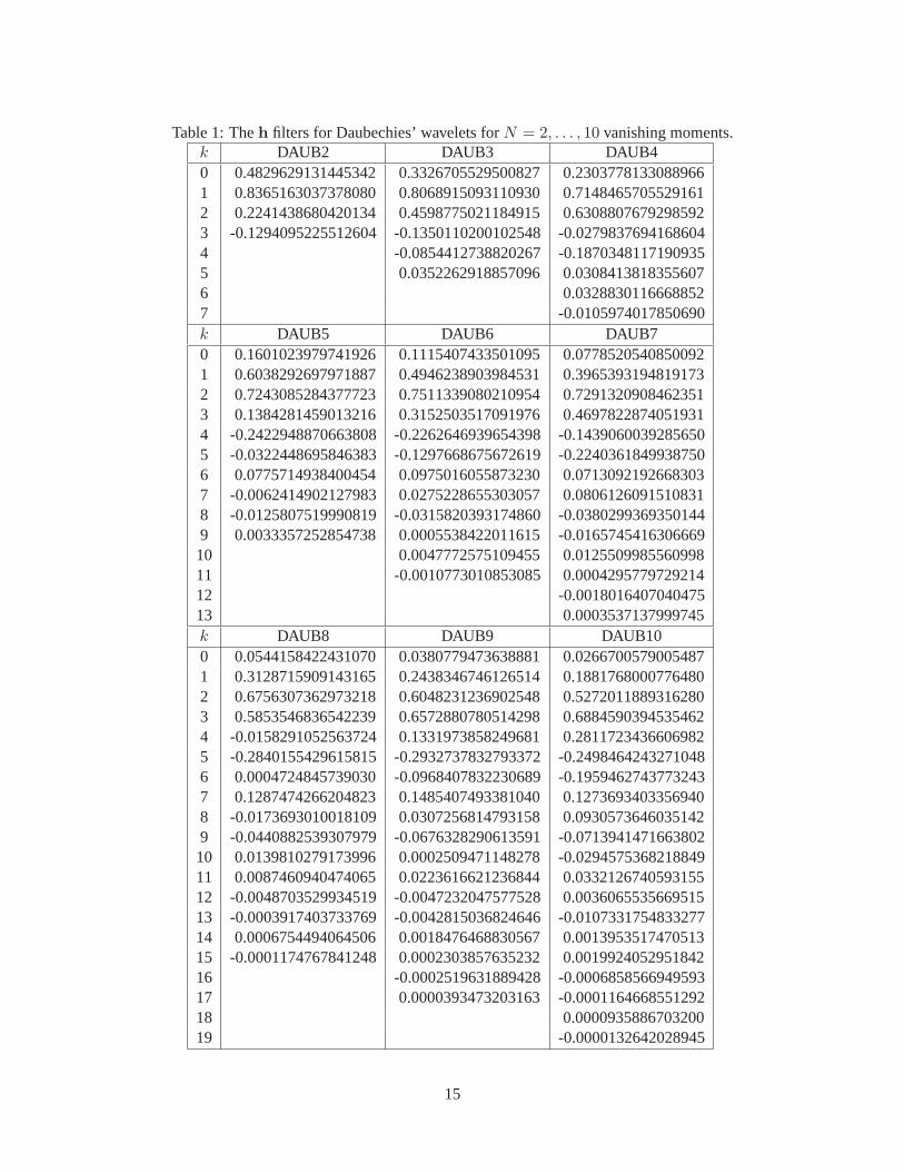
Table 1: Theh filters for Daubechies’ wavelets forN = 2, . . . , 10 vanishing moments.k DAUB2 DAUB3 DAUB40 0.4829629131445342 0.3326705529500827 0.23037781330889661 0.8365163037378080 0.8068915093110930 0.71484657055291612 0.2241438680420134 0.4598775021184915 0.63088076792985923 -0.1294095225512604-0.1350110200102548-0.02798376941686044 -0.0854412738820267-0.18703481171909355 0.0352262918857096 0.03084138183556076 0.03288301166688527 -0.0105974017850690k DAUB5 DAUB6 DAUB70 0.1601023979741926 0.1115407433501095 0.07785205408500921 0.6038292697971887 0.4946238903984531 0.39653931948191732 0.7243085284377723 0.7511339080210954 0.72913209084623513 0.1384281459013216 0.3152503517091976 0.46978228740519314 -0.2422948870663808-0.2262646939654398-0.14390600392856505 -0.0322448695846383-0.1297668675672619-0.22403618499387506 0.0775714938400454 0.0975016055873230 0.07130921926683037 -0.0062414902127983 0.0275228655303057 0.08061260915108318 -0.0125807519990819-0.0315820393174860-0.03802993693501449 0.0033357252854738 0.0005538422011615 -0.016574541630666910 0.0047772575109455 0.012550998556099811 -0.0010773010853085 0.000429577972921412 -0.001801640704047513 0.0003537137999745k DAUB8 DAUB9 DAUB100 0.0544158422431070 0.0380779473638881 0.02667005790054871 0.3128715909143165 0.2438346746126514 0.18817680007764802 0.6756307362973218 0.6048231236902548 0.52720118893162803 0.5853546836542239 0.6572880780514298 0.68845903945354624 -0.0158291052563724 0.1331973858249681 0.28117234366069825 -0.2840155429615815-0.2932737832793372-0.24984642432710486 0.0004724845739030 -0.0968407832230689-0.19594627437732437 0.1287474266204823 0.1485407493381040 0.12736934033569408 -0.0173693010018109 0.0307256814793158 0.09305736460351429 -0.0440882539307979-0.0676328290613591-0.071394147166380210 0.0139810279173996 0.0002509471148278 -0.029457536821884911 0.0087460940474065 0.0223616621236844 0.033212674059315512 -0.0048703529934519-0.0047232047577528 0.003606553566951513 -0.0003917403733769-0.0042815036824646-0.010733175483327714 0.0006754494064506 0.0018476468830567 0.001395351747051315 -0.0001174767841248 0.0002303857635232 0.001992405295184216 -0.0002519631889428-0.000685856694959317 0.0000393473203163 -0.000116466855129218 0.000093588670320019 -0.0000132642028945

15

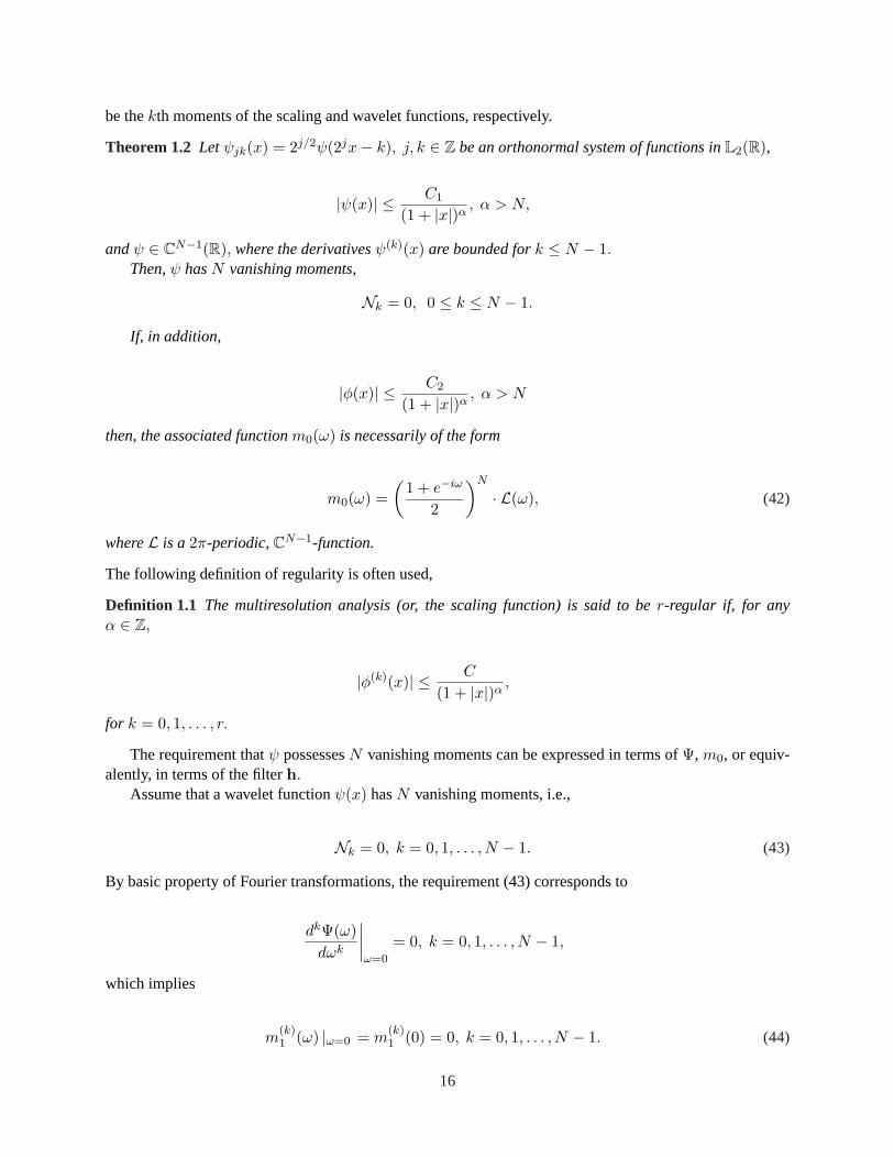
be thekth moments of the scaling and wavelet functions, respectively.

Theorem 1.2 Letψjk(x) = 2j/2ψ(2jx− k), j, k ∈ Z be an orthonormal system of functions inL2(R),

|ψ(x)| ≤ C1

(1 + |x|)α, α > N,

andψ ∈ CN−1(R), where the derivativesψ(k)(x) are bounded fork ≤ N − 1.Then,ψ hasN vanishing moments,

Nk = 0, 0 ≤ k ≤ N − 1.

If, in addition,

|φ(x)| ≤ C2

(1 + |x|)α, α > N

then, the associated functionm0(ω) is necessarily of the form

m0(ω) =(

1 + e−iω

2

)N

· L(ω), (42)

whereL is a2π-periodic,CN−1-function.

The following definition of regularity is often used,

Definition 1.1 The multiresolution analysis (or, the scaling function) is said to ber-regular if, for anyα ∈ Z,

|φ(k)(x)| ≤ C

(1 + |x|)α,

for k = 0, 1, . . . , r.

The requirement thatψ possessesN vanishing moments can be expressed in terms ofΨ, m0, or equiv-alently, in terms of the filterh.

Assume that a wavelet functionψ(x) hasN vanishing moments, i.e.,

Nk = 0, k = 0, 1, . . . , N − 1. (43)

By basic property of Fourier transformations, the requirement (43) corresponds to

dkΨ(ω)dωk

∣∣∣∣ω=0

= 0, k = 0, 1, . . . , N − 1,

which implies

m(k)1 (ω) |ω=0 = m

(k)1 (0) = 0, k = 0, 1, . . . , N − 1. (44)

16

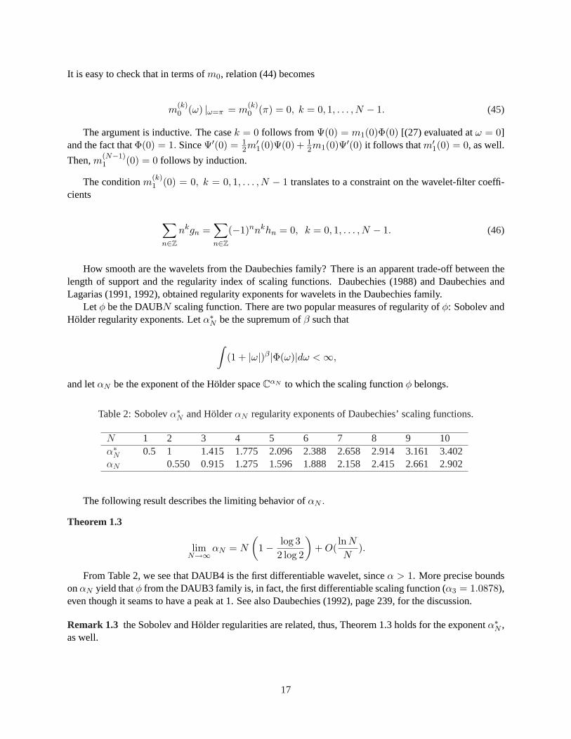
It is easy to check that in terms ofm0, relation (44) becomes

m(k)0 (ω) |ω=π = m

(k)0 (π) = 0, k = 0, 1, . . . , N − 1. (45)

The argument is inductive. The casek = 0 follows fromΨ(0) = m1(0)Φ(0) [(27) evaluated atω = 0]and the fact thatΦ(0) = 1. SinceΨ′(0) = 1

2m′1(0)Ψ(0) + 1

2m1(0)Ψ′(0) it follows thatm′1(0) = 0, as well.

Then,m(N−1)1 (0) = 0 follows by induction.

The conditionm(k)1 (0) = 0, k = 0, 1, . . . , N − 1 translates to a constraint on the wavelet-filter coeffi-

cients

∑

n∈Znkgn =

∑

n∈Z(−1)nnkhn = 0, k = 0, 1, . . . , N − 1. (46)

How smooth are the wavelets from the Daubechies family? There is an apparent trade-off between thelength of support and the regularity index of scaling functions. Daubechies (1988) and Daubechies andLagarias (1991, 1992), obtained regularity exponents for wavelets in the Daubechies family.

Let φ be the DAUBN scaling function. There are two popular measures of regularity ofφ: Sobolev andHolder regularity exponents. Letα∗N be the supremum ofβ such that

∫(1 + |ω|)β|Φ(ω)|dω < ∞,

and letαN be the exponent of the Holder spaceCαN to which the scaling functionφ belongs.

Table 2: Sobolevα∗N and HolderαN regularity exponents of Daubechies’ scaling functions.

N 1 2 3 4 5 6 7 8 9 10α∗N 0.5 1 1.415 1.775 2.096 2.388 2.658 2.914 3.161 3.402αN 0.550 0.915 1.275 1.596 1.888 2.158 2.415 2.661 2.902

The following result describes the limiting behavior ofαN .

Theorem 1.3

limN→∞

αN = N

(1− log 3

2 log 2

)+ O(

ln N

N).

From Table 2, we see that DAUB4 is the first differentiable wavelet, sinceα > 1. More precise boundsonαN yield thatφ from the DAUB3 family is, in fact, the first differentiable scaling function (α3 = 1.0878),even though it seams to have a peak at 1. See also Daubechies (1992), page 239, for the discussion.

Remark 1.3 the Sobolev and Holder regularities are related, thus, Theorem 1.3 holds for the exponentα∗N ,as well.

17

1.5 Approximations and Characterizations of Functional Spaces

Any L2(R) functionf can be represented as

f(x) =∑

j,k

djkψjk(x),

and this unique representation corresponds to a multiresolution decompositionL2(R) =⊕∞

j=−∞Wj . Also,for any fixedj0 the decompositionL2(R) = Vj0 ⊕

⊕∞j=j0

Wj corresponds to the representation

f(x) =∑

k

cj0,kφj0,k(x) +∑

j≥j0

∑

k

djkψj,k(x). (47)

The first sum in (47) is an orthogonal projectionPj0 of f onVj0 .In general, it is possible to bound||Pj0f − f || = ||(I − Pj0)f || if the regularities of functionsf andφ

are known.When bothf andφ haven continuous derivatives, there exists a constantC such that

||(I − Pj0)f ||L2 ≤ C · 2−nj0 ||f ||L2 .

A range of important function spaces can be fully characterized by wavelets. We list a few characteri-zations. For example, a functionf belongs to the Holder spaceCs if and only if there is a constantC suchthat in anr-regular MRA (r > s) the wavelet coefficients satisfy

(i) |cj0,k| ≤ C,

(ii) |dj,k| ≤ C · 2−j(s+ 12), j ≥ j0, k ∈ Z . (48)

A functionf belongs to the SobolevWs2(R) space if and only if

∑

j,k

|djk|2 · (1 + 22js) < ∞.

Even the general (non-homogeneous) Besov spaces, can be characterized by moduli of the waveletcoefficients of its elements. For a givenr-regular MRA withr > max{σ, 1}, the following result (seeMeyer 1992, page 200) holds

Theorem 1.4 LetIj be a set of indices so that{ψi, i ∈ Ij} constitutes an o.n. basis of the detail spaceWj .There exist two constantsC ′ ≥ C > 0 such that, for every exponentp ∈ [1,∞], for eachj ∈ Z and forevery elementf(x) =

∑i∈Ij

diψi(x) in Wj ,

C||f ||p ≤ 2j/22−j/p

∑

i∈Ij

|di|p

1/p

≤ C ′||f ||p.

18

The following characterization of BesovBσp,q spaces can be obtained directly from this result. If the MRA

has regularityr > s, then wavelet bases are Riesz bases for all1 ≤ p, q ≤ ∞, 0 < σ < r.The functionf =

∑k cj0kφj0k(x) +

∑j≥j0

∑k djkψjk(x) belongs toBσ

p,q space if its wavelet coeffi-cients satisfy

(∑

k

|cj0,k|p)1/p

< ∞,

and

∑

i∈Ij

2j(σ+1/2−1/p)|di|p

1/p

, j ≥ j0

is an`q sequence, i.e,[∑

j≥j0

(2j(σ+1/2−1/p)(

∑k |dj,k|p)1/p

)q]1/q

< ∞.

The results listed are concerned with global regularity. The local regularity of functions can also bestudied by inspecting the magnitudes of their wavelet coefficients. For more details, we direct the reader tothe work of Jaffard (1991) and Jaffard and Laurencot (1992).

1.5.1 Daubechies-Lagarias Algorithm

As a nice calculational example, we describe an algorithm for fast numerical calculation of wavelet valuesat a given point, based on the Daubechies-Lagarias (Daubechies and Lagarias, 1991, 1992)local pyramidalalgorithm. Thematlab routinesPhi.m andPsi.m in the Matlab sesction implement the algorithm.

The scaling function and wavelet function in Daubechies’ families have no explicit representations (ex-cept for the Haar wavelet). Sometimes, it necessary to find values of DAUB functions at arbitrary points;examples include calculation of coefficients in density estimation and non-equally spaced regression.

The Daubechies-Lagarias algorithm enables us to evaluateφ andψ at a point with preassigned precision.We illustrate the algorithm on wavelets from the Daubechies family; however, the algorithm works for allorthoginal wavelet filters.

Let φ be the scaling function of the DAUBN wavelet. The support ofφ is [0, 2N − 1]. Let x ∈ (0, 1),and letdyad(x) = {d1, d2, . . . dn, . . . } be the set of 0-1 digits in the dyadic representation ofx (x =∑∞

j=1 dj2−j). By dyad(x, n), we denote the subset of the firstn digits fromdyad(x), i.e., dyad(x, n) ={d1, d2, . . . dn}.

Let h = (h0, h1, . . . , h2N−1) be the wavelet filter coefficients. We build two(2N − 1) × (2N − 1)matrices as:

T0 = (√

2 · h2i−j−1)1≤i,j≤2N−1 and T1 = (√

2 · h2i−j)1≤i,j≤2N−1. (49)

Then the local pyramidal algorithm can be constructed based on Theorem 1.5.

19

Theorem 1.5

limn→∞ Td1 · Td2 · · · · · Tdn (50)

=

φ(x) φ(x) . . . φ(x)φ(x + 1) φ(x + 1) . . . φ(x + 1)

...φ(x + 2N − 2) φ(x + 2N − 2) . . . φ(x + 2N − 2)

.

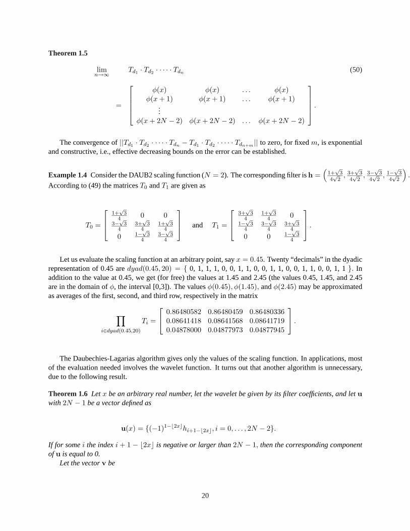
The convergence of||Td1 · Td2 · · · · · Tdn − Td1 · Td2 · · · · · Tdn+m || to zero, for fixedm, is exponentialand constructive, i.e., effective decreasing bounds on the error can be established.

Example 1.4 Consider the DAUB2 scaling function (N = 2). The corresponding filter ish =(

1+√

34√

2, 3+

√3

4√

2, 3−√3

4√

2, 1−√3

4√

2

).

According to (49) the matricesT0 andT1 are given as

T0 =

1+√

34 0 0

3−√34

3+√

34

1+√

34

0 1−√34

3−√34

and T1 =

3+√

34

1+√

34 0

1−√34

3−√34

3+√

34

0 0 1−√34

.

Let us evaluate the scaling function at an arbitrary point, sayx = 0.45. Twenty “decimals” in the dyadicrepresentation of 0.45 aredyad(0.45, 20) = { 0, 1, 1, 1, 0, 0, 1, 1, 0, 0, 1, 1, 0, 0, 1, 1, 0, 0, 1, 1}. Inaddition to the value at 0.45, we get (for free) the values at 1.45 and 2.45 (the values 0.45, 1.45, and 2.45are in the domain ofφ, the interval [0,3]). The valuesφ(0.45), φ(1.45), andφ(2.45) may be approximatedas averages of the first, second, and third row, respectively in the matrix

∏

i∈dyad(0.45,20)

Ti =

0.86480582 0.86480459 0.864803360.08641418 0.08641568 0.086417190.04878000 0.04877973 0.04877945

.

The Daubechies-Lagarias algorithm gives only the values of the scaling function. In applications, mostof the evaluation needed involves the wavelet function. It turns out that another algorithm is unnecessary,due to the following result.

Theorem 1.6 Letx be an arbitrary real number, let the wavelet be given by its filter coefficients, and letuwith 2N − 1 be a vector defined as

u(x) = {(−1)1−b2xchi+1−b2xc, i = 0, . . . , 2N − 2}.

If for somei the indexi + 1 − b2xc is negative or larger than2N − 1, then the corresponding componentof u is equal to 0.

Let the vectorv be

20

v(x, n) =1

2N − 11′

∏

i∈dyad({2x},n)

Ti,

where1′ = (1, 1, . . . , 1) is the row-vector of ones. Then,

ψ(x) = limn→∞u(x)′v(x, n),

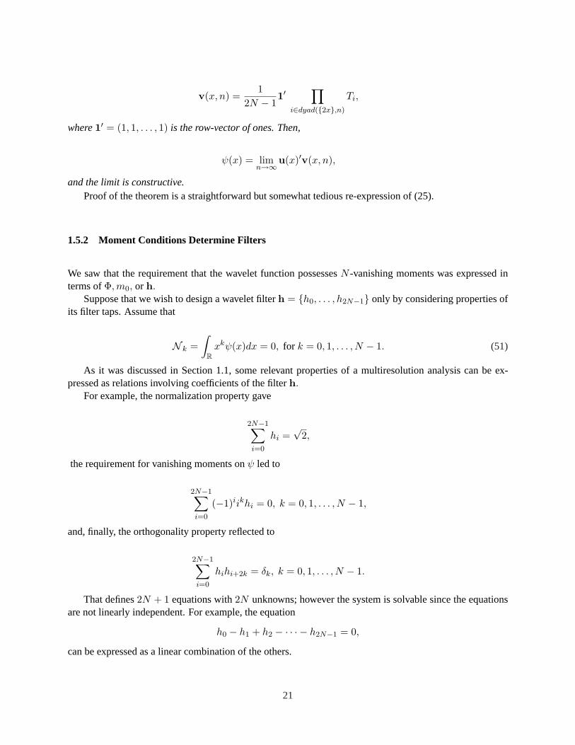
and the limit is constructive.Proof of the theorem is a straightforward but somewhat tedious re-expression of (25).

1.5.2 Moment Conditions Determine Filters

We saw that the requirement that the wavelet function possessesN -vanishing moments was expressed interms ofΦ,m0, or h.

Suppose that we wish to design a wavelet filterh = {h0, . . . , h2N−1} only by considering properties ofits filter taps. Assume that

N k =∫

Rxkψ(x)dx = 0, for k = 0, 1, . . . , N − 1. (51)

As it was discussed in Section 1.1, some relevant properties of a multiresolution analysis can be ex-pressed as relations involving coefficients of the filterh.

For example, the normalization property gave

2N−1∑

i=0

hi =√

2,

the requirement for vanishing moments onψ led to

2N−1∑

i=0

(−1)iikhi = 0, k = 0, 1, . . . , N − 1,

and, finally, the orthogonality property reflected to

2N−1∑

i=0

hihi+2k = δk, k = 0, 1, . . . , N − 1.

That defines2N + 1 equations with2N unknowns; however the system is solvable since the equationsare not linearly independent. For example, the equation

h0 − h1 + h2 − · · · − h2N−1 = 0,

can be expressed as a linear combination of the others.

21

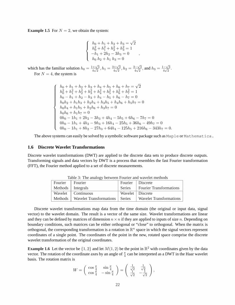
Example 1.5 ForN = 2, we obtain the system:

h0 + h1 + h2 + h3 =√

2h2

0 + h21 + h2

2 + h23 = 1

−h1 + 2h2 − 3h3 = 0 ,h0 h2 + h1 h3 = 0

which has the familiar solutionh0 = 1+√

34√

2, h1 = 3+

√3

4√

2, h2 = 3−√3

4√

2, andh3 = 1−√3

4√

2.

ForN = 4, the system is

h0 + h1 + h2 + h3 + h4 + h5 + h6 + h7 =√

2h2

0 + h21 + h2

2 + h23 + h2

4 + h25 + h2

6 + h27 = 1

h0 − h1 + h2 − h3 + h4 − h5 + h6 − h7 = 0h0h2 + h1h3 + h2h4 + h3h5 + h4h6 + h5h7 = 0h0h4 + h1h5 + h2h6 + h3h7 = 0h0h6 + h1h7 = 00h0 − 1h1 + 2h2 − 3h3 + 4h4 − 5h5 + 6h6 − 7h7 = 00h0 − 1h1 + 4h2 − 9h3 + 16h4 − 25h5 + 36h6 − 49h7 = 00h0 − 1h1 + 8h2 − 27h3 + 64h4 − 125h5 + 216h6 − 343h7 = 0.

The above systems can easily be solved by a symbolic software package such asMaple orMathematica.

1.6 Discrete Wavelet Transformations

Discrete wavelet transformations (DWT) are applied to the discrete data sets to produce discrete outputs.Transforming signals and data vectors by DWT is a process that resembles the fast Fourier transformation(FFT), the Fourier method applied to a set of discrete measurements.

Table 3: The analogy between Fourier and wavelet methodsFourier Fourier Fourier DiscreteMethods Integrals Series Fourier TransformationsWavelet Continuous Wavelet DiscreteMethods Wavelet Transformations Series Wavelet Transformations

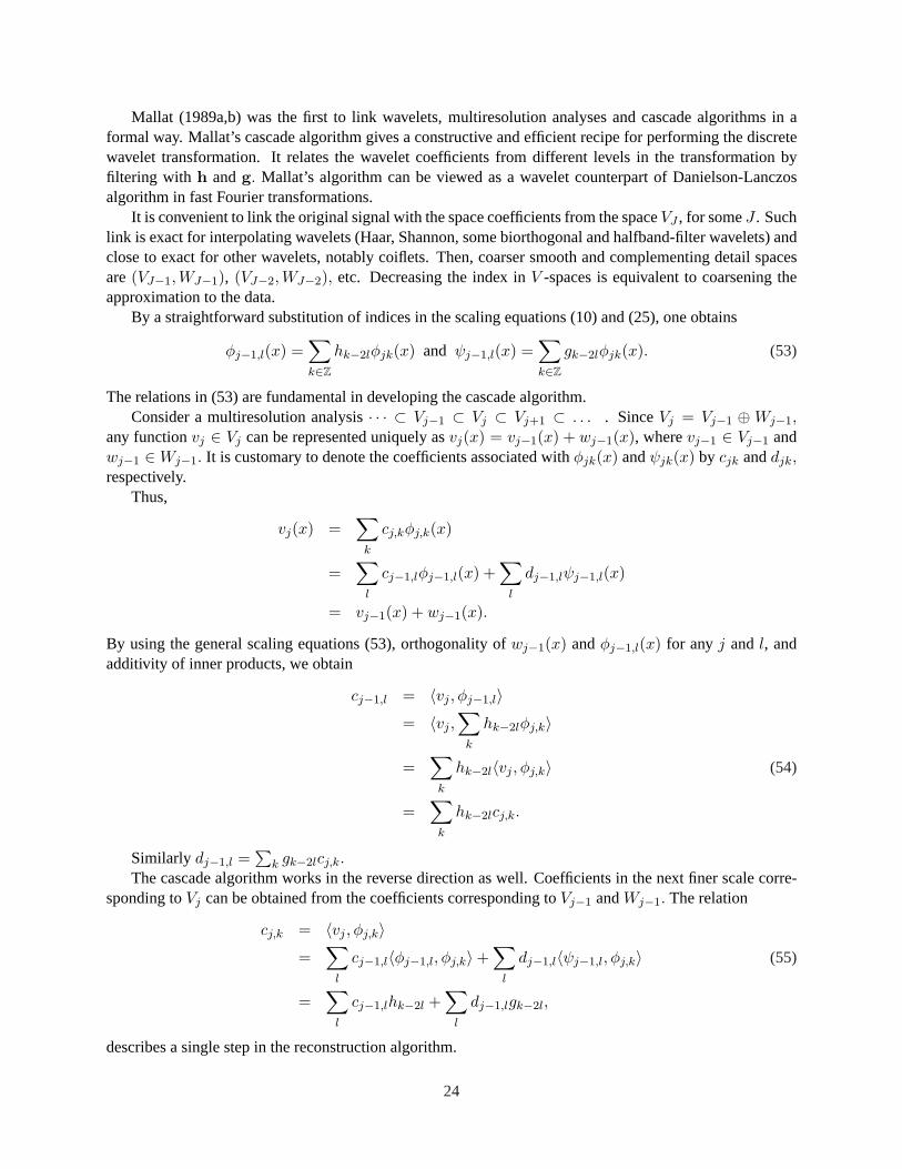
Discrete wavelet transformations map data from the time domain (the original or input data, signalvector) to the wavelet domain. The result is a vector of the same size. Wavelet transformations are linearand they can be defined by matrices of dimensionn×n if they are applied to inputs of sizen. Depending onboundary conditions, such matrices can be either orthogonal or “close” to orthogonal. When the matrix isorthogonal, the corresponding transformation is a rotation inRn space in which the signal vectors representcoordinates of a single point. The coordinates of the point in the new, rotated space comprise the discretewavelet transformation of the original coordinates.

Example 1.6 Let the vector be{1, 2} and letM(1, 2) be the point inR2 with coordinates given by the datavector. The rotation of the coordinate axes by an angle ofπ

4 can be interpreted as a DWT in the Haar waveletbasis. The rotation matrix is

W =(

cos π4 sin π

4cos π

4 − sin π4

)=

(1√2

1√2

1√2

− 1√2

),

22

and the discrete wavelet transformation of(1, 2)′ is W · (1, 2)′ = ( 3√2,− 1√

2)′. Notice thatthe energy

(squared distance of the point from the origin) is preserved,12 + 22 = (12)2 + (

√3

2 )2, sinceW is a rotation.

Example 1.7 Let y = (1, 0,−3, 2, 1, 0, 1, 2). If Haar wavelet is used, the valuesf(n) = yn, n =0, 1, . . . , 7 are interpolated by the father wavelet, the vector represent the sampled piecewise constant func-tion. It is obvious that such definedf belongs to Haar’s multiresolution spaceV0.

The following matrix equation gives the connection betweeny and the wavelet coefficients (data in thewavelet domain).

10−321012

=

12√

21

2√

212 0 1√

20 0 0

12√

21

2√

212 0 − 1√

20 0 0

12√

21

2√

2−1

2 0 0 1√2

0 01

2√

21

2√

2−1

2 0 0 − 1√2

0 01

2√

2− 1

2√

20 1

2 0 0 1√2

01

2√

2− 1

2√

20 1

2 0 0 − 1√2

01

2√

2− 1

2√

20 −1

2 0 0 0 1√2

12√

2− 1

2√

20 −1

2 0 0 0 − 1√2

·

c00

d00

d10

d11

d20

d21

d22

d23

.

The solution is

c00

d00

d10

d11

d20

d21

d22

d23

=

√2

−√21−11√2

− 5√2

1√2

− 1√2

.

Thus,

f =√

2φ−3,0 −√

2ψ−3,0 + ψ−2,0 − ψ−2,1

+1√2ψ−1,0 − 5√

2ψ−1,1 +

1√2ψ−1,2 − 1√

2ψ−1,3. (52)

The solution is easy to verify. For example, whenx ∈ [0, 1),

f(x) =√

2 · 12√

2−√

2 · 12√

2+ 1 · 1

2+

1√2· 1√

2= 1/2 + 1/2 = 1 (= y0).

Performing wavelet transformations by multiplying the input vector with an appropriate orthogonal ma-trix is conceptually straightforward, but of limited practical value. Storing and manipulating transformationmatrices when inputs are long(> 2000) may not even be feasible.

In the context of image processing, Burt and Adelson (1982a,b) developed orthogonal and biorthogonalpyramid algorithms. Pyramid or cascade procedures process an image at different scales, ranging from fineto coarse, in a tree-like algorithm. The images can be denoised, enhanced or compressed by appropriatescale-wise treatments.

23

Mallat (1989a,b) was the first to link wavelets, multiresolution analyses and cascade algorithms in aformal way. Mallat’s cascade algorithm gives a constructive and efficient recipe for performing the discretewavelet transformation. It relates the wavelet coefficients from different levels in the transformation byfiltering with h andg. Mallat’s algorithm can be viewed as a wavelet counterpart of Danielson-Lanczosalgorithm in fast Fourier transformations.

It is convenient to link the original signal with the space coefficients from the spaceVJ , for someJ . Suchlink is exact for interpolating wavelets (Haar, Shannon, some biorthogonal and halfband-filter wavelets) andclose to exact for other wavelets, notably coiflets. Then, coarser smooth and complementing detail spacesare(VJ−1,WJ−1), (VJ−2,WJ−2), etc. Decreasing the index inV -spaces is equivalent to coarsening theapproximation to the data.

By a straightforward substitution of indices in the scaling equations (10) and (25), one obtains

φj−1,l(x) =∑

k∈Zhk−2lφjk(x) and ψj−1,l(x) =

∑

k∈Zgk−2lφjk(x). (53)

The relations in (53) are fundamental in developing the cascade algorithm.Consider a multiresolution analysis· · · ⊂ Vj−1 ⊂ Vj ⊂ Vj+1 ⊂ . . . . SinceVj = Vj−1 ⊕ Wj−1,

any functionvj ∈ Vj can be represented uniquely asvj(x) = vj−1(x) + wj−1(x), wherevj−1 ∈ Vj−1 andwj−1 ∈ Wj−1. It is customary to denote the coefficients associated withφjk(x) andψjk(x) by cjk anddjk,respectively.

Thus,

vj(x) =∑

k

cj,kφj,k(x)

=∑

l

cj−1,lφj−1,l(x) +∑

l

dj−1,lψj−1,l(x)

= vj−1(x) + wj−1(x).

By using the general scaling equations (53), orthogonality ofwj−1(x) andφj−1,l(x) for any j and l, andadditivity of inner products, we obtain

cj−1,l = 〈vj , φj−1,l〉= 〈vj ,

∑

k

hk−2lφj,k〉

=∑

k

hk−2l〈vj , φj,k〉 (54)

=∑

k

hk−2lcj,k.

Similarly dj−1,l =∑

k gk−2lcj,k.The cascade algorithm works in the reverse direction as well. Coefficients in the next finer scale corre-

sponding toVj can be obtained from the coefficients corresponding toVj−1 andWj−1. The relation

cj,k = 〈vj , φj,k〉=

∑

l

cj−1,l〈φj−1,l, φj,k〉+∑

l

dj−1,l〈ψj−1,l, φj,k〉 (55)

=∑

l

cj−1,lhk−2l +∑

l

dj−1,lgk−2l,

describes a single step in the reconstruction algorithm.

24

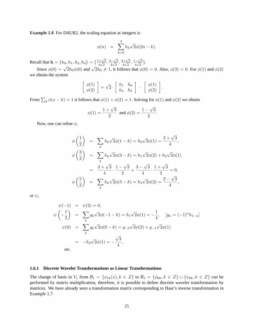
Example 1.8 For DAUB2, the scaling equation at integers is

φ(n) =3∑

k=0

hk

√2φ(2n− k).

Recall thath = {h0, h1, h2, h3} = {1+√

34√

2, 3−√3

4√

2, 3+

√3

4√

2, 1−√3

4√

2}.

Sinceφ(0) =√

2h0φ(0) and√

2h0 6= 1, it follows thatφ(0) = 0. Also, φ(3) = 0. For φ(1) andφ(2)we obtain the system

[φ(1)φ(2)

]=√

2 ·[

h1 h0

h3 h2

]·

[φ(1)φ(2)

].

From∑

k φ(x− k) = 1 it follows thatφ(1) + φ(2) = 1. Solving forφ(1) andφ(2) we obtain

φ(1) =1 +

√3

2andφ(2) =

1−√32

.

Now, one can refineφ,

φ

(12

)=

∑

k

hk

√2φ(1− k) = h0

√2φ(1) =

2 +√

34

,

φ

(32

)=

∑

k

hk

√2φ(3− k) = h1

√2φ(2) + h2

√2φ(1)

=3 +

√3

4· 1−√3

2+

3−√34

· 1 +√

32

= 0,

φ

(52

)=

∑

k

hk

√2φ(5− k) = h3

√2φ(2) =

2−√34

,

or ψ,

ψ(−1) = ψ(2) = 0,

ψ

(−1

2

)=

∑

k

gk

√2φ(−1− k) = h1

√2φ(1) = −1

4, [gn = (−1)nh1−n]

ψ(0) =∑

k

gk

√2φ(0− k) = g−2

√2φ(2) + g−1

√2φ(1)

= −h2

√2φ(1) = −

√3

4,

etc.

1.6.1 Discrete Wavelet Transformations as Linear Transformations

The change of basis inV1 from B1 = {φ1k(x), k ∈ Z} to B2 = {φ0k, k ∈ Z} ∪ {ψ0k, k ∈ Z} can beperformed by matrix multiplication, therefore, it is possible to define discrete wavelet transformation bymatrices. We have already seen a transformation matrix corresponding to Haar’s inverse transformation inExample 1.7.

25

Let the length of the input signal be2J , and leth = {hs, s ∈ Z} be the wavelet filter and letN be anappropriately chosen constant.

Denote byHk is a matrix of size(2J−k × 2J−k+1), k = 1, . . . with entries

hs, s = (N − 1) + (i− 1)− 2(j − 1) modulo2J−k+1, (56)

at the position(i, j).Note thatHk is a circulant matrix, itsith row is1st row circularly shifted to the right by2(i− 1) units.

This circularity is a consequence of using themodulooperator in (56).By analogy, define a matrixGk by using the filterg. A version ofGk corresponding to the already

definedHk can be obtained by changinghi by (−1)ihN+1−i. The constantN is a shift parameter andaffects the position of the wavelet on the time scale. For filters from the Daubechies family, standard choicefor N is the number of vanishing moments. See also Remark 1.2.

The matrix

[Hk

Gk

]is a basis-change matrix in2J−k+1 dimensional space; consequently, it is unitary.

Therefore,

I2J−k = [H ′k G′

k][

Hk

Gk

]= H ′

k ·Hk + G′k ·Gk.

and

I =[

Hk

Gk

]· [H ′

k G′k] =

[Hk ·H ′

k Hk ·G′k

Gk ·H ′k Gk ·G′

k

].

That implies,

Hk ·H ′k = I, Gk ·G′

k = I, Gk ·H ′k = Hk ·G′

k = 0, andH ′k ·Hk + G′

k ·Gk = I.

Now, for a sequencey theJ-step wavelet transformation isd = WJ · y, where

W1 =[

H1

G1

], W2 =

[H2

G2

]·H1

G1

,

W3 =

[H3

G3

]·H2

G2

·H1

G1

, . . .

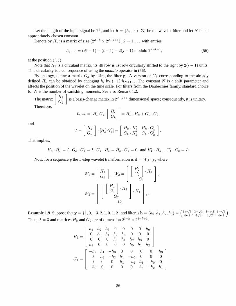
Example 1.9 Suppose thaty = {1, 0,−3, 2, 1, 0, 1, 2} and filter ish = (h0, h1, h2, h3) =(

1+√

34√

2, 3+

√3

4√

2, 3−√3

4√

2, 1−√3

4√

2

).

Then,J = 3 and matricesHk andGk are of dimension23−k × 23−k+1.

H1 =

h1 h2 h3 0 0 0 0 h0

0 h0 h1 h2 h3 0 0 00 0 0 h0 h1 h2 h3 0h3 0 0 0 0 h0 h1 h2

G1 =

−h2 h1 −h0 0 0 0 0 h3

0 h3 −h2 h1 −h0 0 0 00 0 0 h3 −h2 h1 −h0 0−h0 0 0 0 0 h3 −h2 h1

.

26

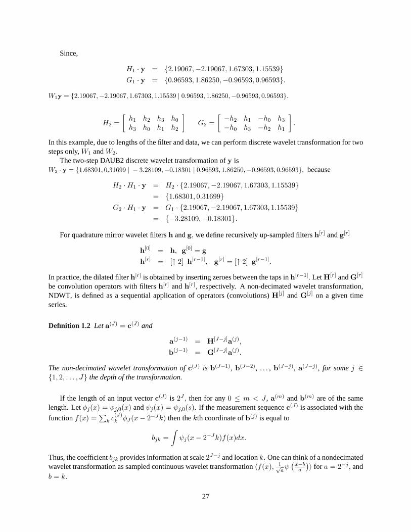
Since,

H1 · y = {2.19067,−2.19067, 1.67303, 1.15539}G1 · y = {0.96593, 1.86250,−0.96593, 0.96593}.

W1y = {2.19067,−2.19067, 1.67303, 1.15539 | 0.96593, 1.86250,−0.96593, 0.96593}.

H2 =[

h1 h2 h3 h0

h3 h0 h1 h2

]G2 =

[ −h2 h1 −h0 h3

−h0 h3 −h2 h1

].

In this example, due to lengths of the filter and data, we can perform discrete wavelet transformation for twosteps only,W1 andW2.

The two-step DAUB2 discrete wavelet transformation ofy isW2 · y = {1.68301, 0.31699 | − 3.28109,−0.18301 | 0.96593, 1.86250,−0.96593, 0.96593}, because

H2 ·H1 · y = H2 · {2.19067,−2.19067, 1.67303, 1.15539}= {1.68301, 0.31699}

G2 ·H1 · y = G1 · {2.19067,−2.19067, 1.67303, 1.15539}= {−3.28109,−0.18301}.

For quadrature mirror wavelet filtersh andg, we define recursively up-sampled filtersh[r] andg[r]

h[0] = h, g[0] = g

h[r] = [↑ 2] h[r−1], g[r] = [↑ 2] g[r−1].

In practice, the dilated filterh[r] is obtained by inserting zeroes between the taps inh[r−1]. LetH[r] andG[r]

be convolution operators with filtersh[r] andh[r], respectively. A non-decimated wavelet transformation,NDWT, is defined as a sequential application of operators (convolutions)H[j] andG[j] on a given timeseries.

Definition 1.2 Leta(J) = c(J) and

a(j−1) = H[J−j]a(j),

b(j−1) = G[J−j]a(j).

The non-decimated wavelet transformation ofc(J) is b(J−1), b(J−2), . . . , b(J−j), a(J−j), for somej ∈{1, 2, . . . , J} the depth of the transformation.

If the length of an input vectorc(J) is 2J , then for any0 ≤ m < J , a(m) andb(m) are of the samelength. Letφj(x) = φj,0(x) andψj(x) = ψj,0(s). If the measurement sequencec(J) is associated with the

functionf(x) =∑

k c(J)k φJ(x− 2−Jk) then thekth coordinate ofb(j) is equal to

bjk =∫

ψj(x− 2−Jk)f(x)dx.

Thus, the coefficientbjk provides information at scale2J−j and locationk. One can think of a nondecimatedwavelet transformation as sampled continuous wavelet transformation〈f(x), 1√

aψ

(x−ba

)〉 for a = 2−j , andb = k.

27