1 A Universal Task: Finding Hay in a Haystack Given circuit C: {0,1} n →{0,1} with μ( C) ≥ ½,...
88
1 A Universal Task: Finding Hay in a Haystack Given circuit C: {0,1} n →{0,1} with μ(C) ≥ ½ , find x so that C(x)=1. Want: Algorithm polynomial in n and size of C.
-
date post
21-Dec-2015 -
Category
Documents
-
view
214 -
download
0
Transcript of 1 A Universal Task: Finding Hay in a Haystack Given circuit C: {0,1} n →{0,1} with μ( C) ≥ ½,...
1
A Universal Task: Finding Hay in a Haystack
Given circuit C: {0,1}n →{0,1} with μ(C) ≥ ½ , find x so that C(x)=1.
Want: Algorithm polynomial in n and size of C.
2
Hypothesis H
There exists deterministic polytime procedure findHay taking as input a circuit C: {0,1}n →{0,1} so that
1. findHay(C) is in {0,1}n.
2. If μ(C) ≥ ½ then C(findHay(C))=1.
3
Robustness of Hypothesis H
The constant ½ can be replaced with• any constant strictly between 0 and 1,• n-k (quite close to 0), or• 1-2-n1- (very close to 1),without changing truth value of Hypothesis H.
To get even closer to 1, we should try to reduce error probability using few random bits. This question can be considered even in black-box model.
4
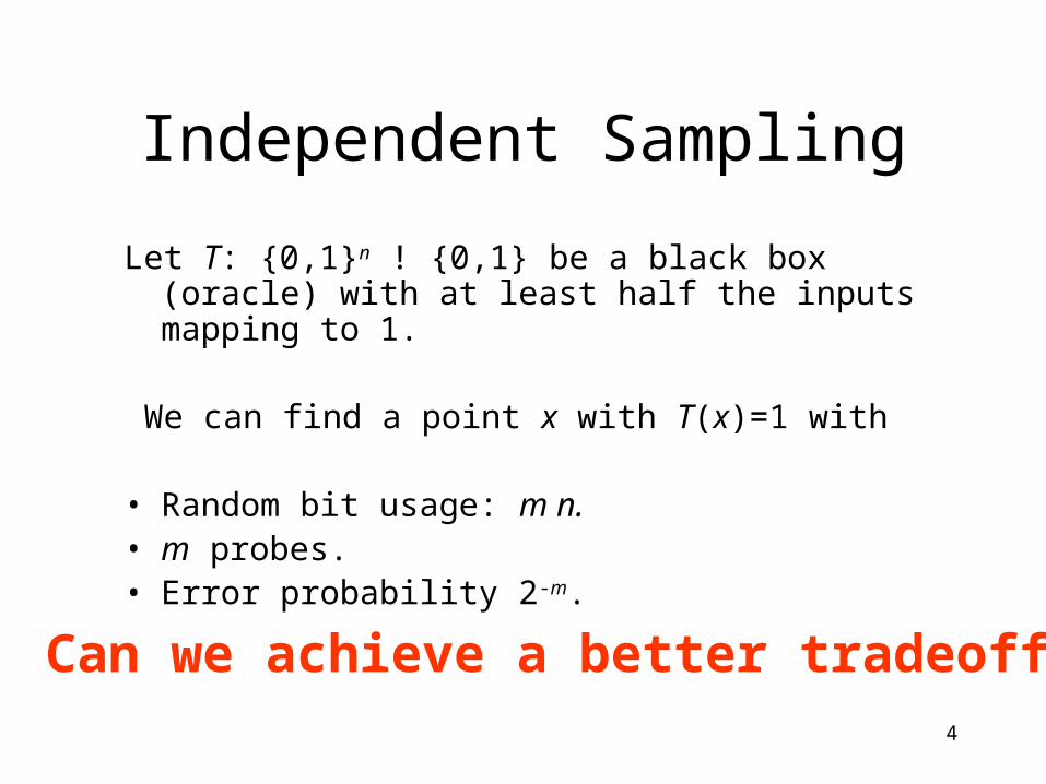
Independent Sampling
Let T: {0,1}n ! {0,1} be a black box (oracle) with at least half the inputs mapping to 1.
We can find a point x with T(x)=1 with
• Random bit usage: m n.• m probes.• Error probability 2-m.
Can we achieve a better tradeoff?
5
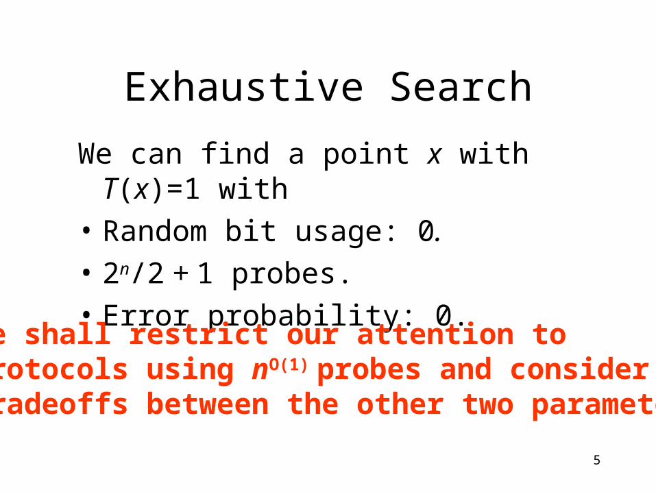
Exhaustive Search
We can find a point x with T(x)=1 with
• Random bit usage: 0.
• 2n/2 + 1 probes.
• Error probability: 0.
We shall restrict our attention to protocols using nO(1) probes and considertradeoffs between the other two parameters.
6
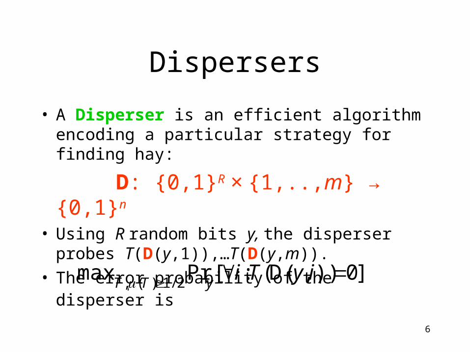
Dispersers
• A Disperser is an efficient algorithm encoding a particular strategy for finding hay:
D: {0,1}R × {1,..,m} → {0,1}n
• Using R random bits y, the disperser probes T(D(y,1)),…T(D(y,m)).
• The error probability of the disperser is ]0)),(D(:[Prmax
2/1)(, iyTi
yTT
7
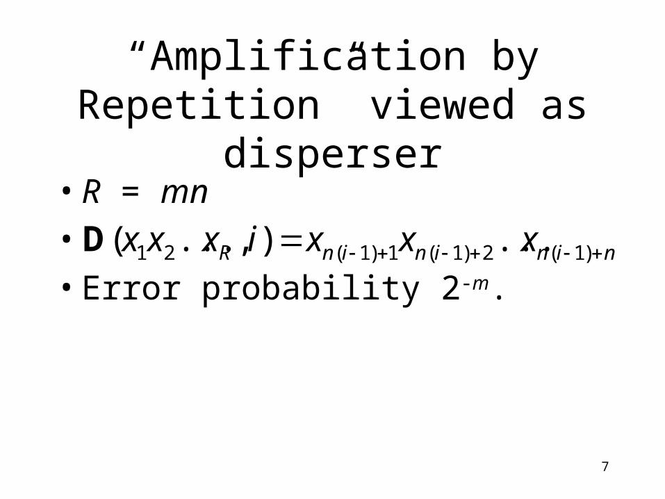
“Amplification by Repetition” viewed as disperser
• R = mn
•
• Error probability 2-m.ninininR xxxixxx )1(2)1(1)1(21 ...),...(D

8
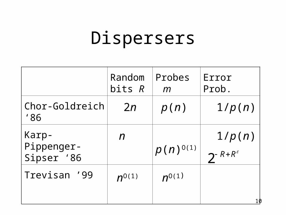
Dispersers
Random bits R
Probes m
Error Prob.
Chor-Goldreich ‘86 2n p(n) 1/p(n)
Karp-Pippenger-Sipser ‘86
n p(n)O(1) 1/p(n)
Trevisan ’99 nO(1) nO(1) RR2
9
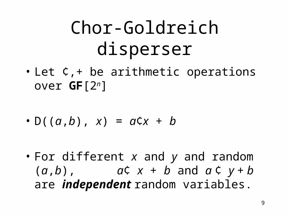
Chor-Goldreich disperser
• Let ¢,+ be arithmetic operations over GF[2n]
• D((a,b), x) = a¢x + b
• For different x and y and random (a,b), a¢ x + b and a ¢ y + b are independent random variables.
10
Dispersers
Random bits R
Probes m
Error Prob.
Chor-Goldreich ‘86 2n p(n) 1/p(n)
Karp-Pippenger-Sipser ‘86
n p(n)O(1) 1/p(n)
Trevisan ’99 nO(1) nO(1) RR2
11
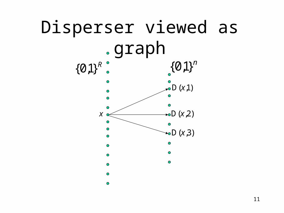
Disperser viewed as graphR}1,0{
n}1,0{
x
)1,(D x
)2,(D x
)3,(D x
12
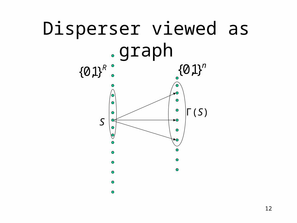
Disperser viewed as graphR}1,0{
n}1,0{
SΓ(S)
13
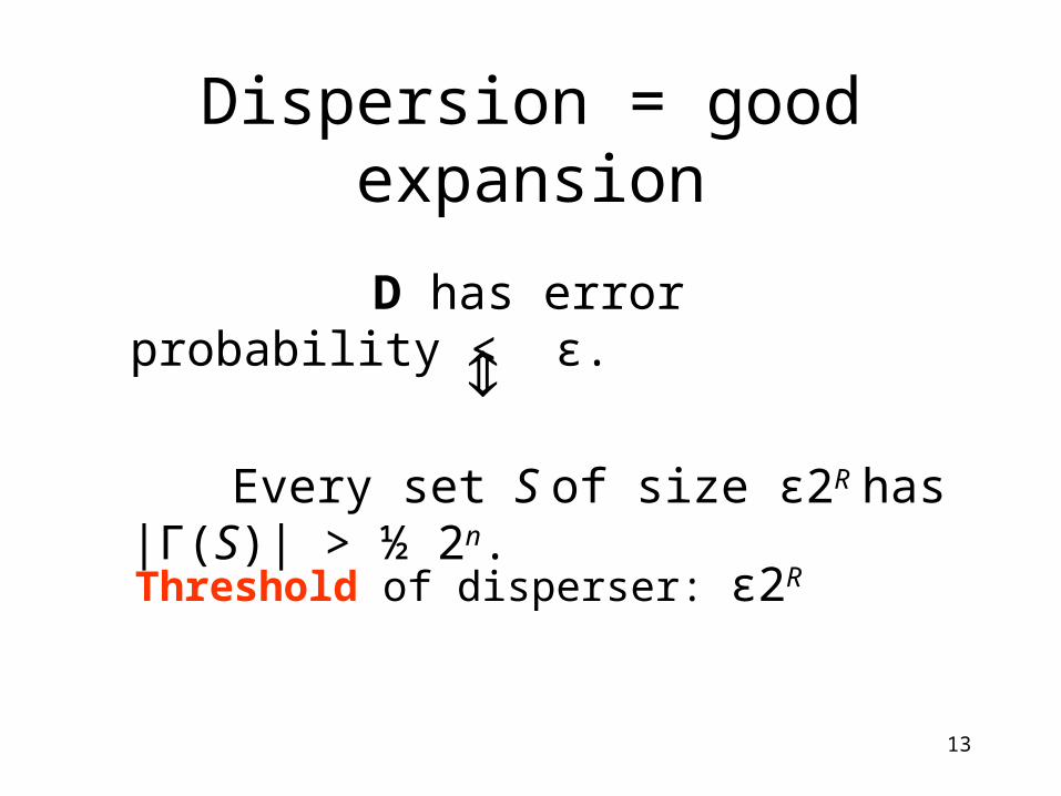
Dispersion = good expansion
D has error probability < ε.
Every set S of size ε2R has |Γ(S)| > ½ 2n.
⇕
Threshold of disperser: ε2R
14
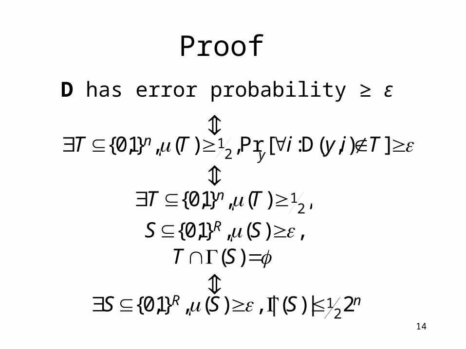
Proof
D has error probability ≥ ε
]),(D:[Pr,)(,}1,0{ 21 TiyiTT
yn
)(,)(,}1,0{
,)(,}1,0{ 21
STSS
TTR
n
nR SSS 2|)(,|)(,}1,0{ 21
⇕
⇕
⇕

15
Dispersers
Random bits R
Probes m
Error Prob.
Chor-Goldreich ‘86 2n p(n) 1/p(n)
Karp-Pippenger-Sipser ‘86
n p(n)O(1) 1/p(n)
Trevisan ’99 nO(1) nO(1) RR2
16
Karp-Pippenger-Sipser disperser
• Let G be a constant degree explicit expander graph on {0,1}n.
• D(x, s) = y for some s if and only if the distance between x and y in G is at most c log n.

17
Dispersers
Random bits R
Probes m
Error Prob.
Chor-Goldreich ‘86 2n p(n) 1/p(n)
Karp-Pippenger-Sipser ‘86
n p(n)O(1) 1/p(n)
Trevisan ’99 nO(1) nO(1) RR2
18
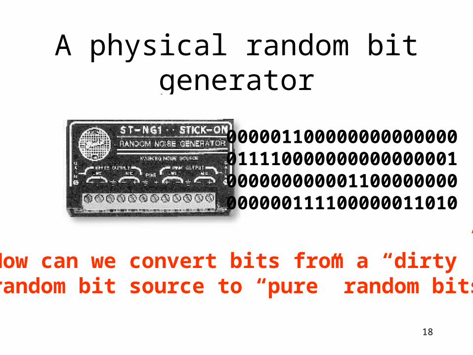
A physical random bit generator
How can we convert bits from a “dirty” random bit source to “pure” random bits?
000001100000000000000011110000000000000001000000000001100000000000000111100000011010
19
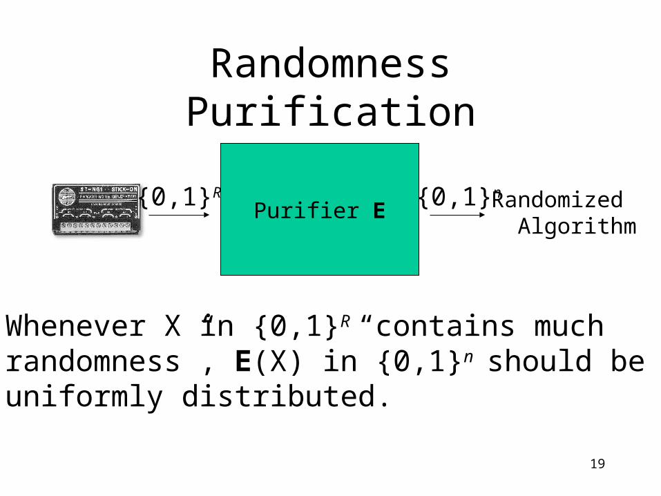
Randomness Purification
Purifier E{0,1}R {0,1}n Randomized
Algorithm
Whenever X in {0,1}R “contains much randomness”, E(X) in {0,1}n should be uniformly distributed.
20
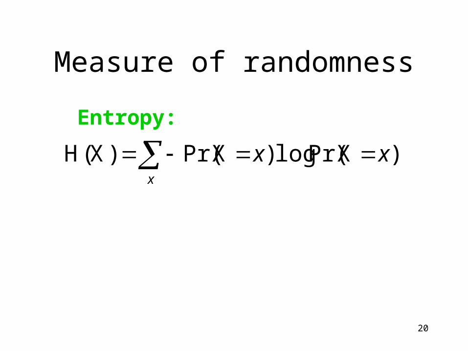
Measure of randomness
Entropy:
)XPr(log)XPr()X(H xxx
21
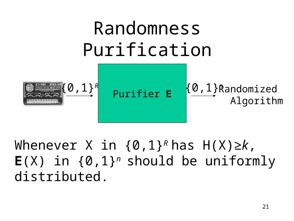
Randomness Purification
Purifier E{0,1}R {0,1}n Randomized
Algorithm
Whenever X in {0,1}R has H(X)≥k, E(X) in {0,1}n should be uniformly distributed.
22
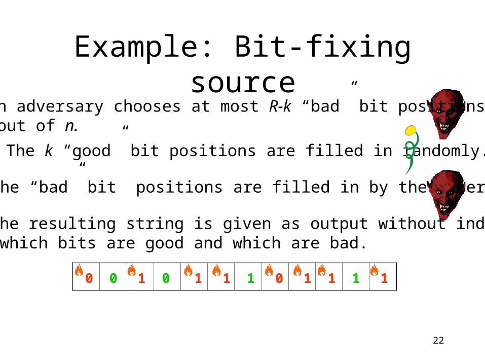
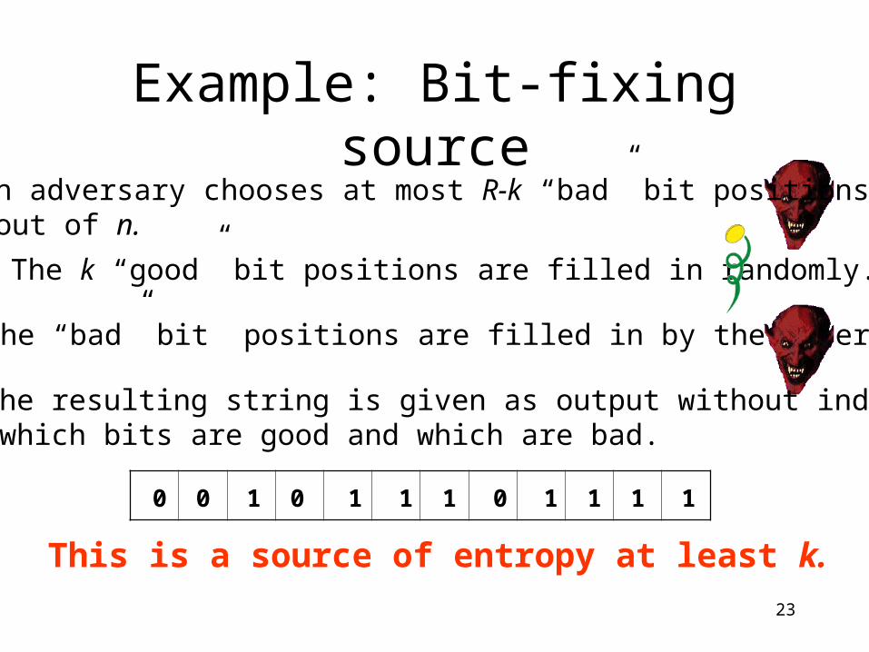
Example: Bit-fixing source1. An adversary chooses at most R-k “bad” bit positions out of n.
2. The k “good” bit positions are filled in randomly.
3. The “bad” bit positions are filled in by the adversary.
10 0 10 1 1 1 0 1 1 1
4. The resulting string is given as output without indicating which bits are good and which are bad.
23
Example: Bit-fixing source1. An adversary chooses at most R-k “bad” bit positions out of n.
2. The k “good” bit positions are filled in randomly.
3. The “bad” bit positions are filled in by the adversary.
This is a source of entropy at least k.
10 0 10 1 1 1 0 1 1 1
4. The resulting string is given as output without indicating which bits are good and which are bad.
24
Randomness Purifiers don’t exist!
25
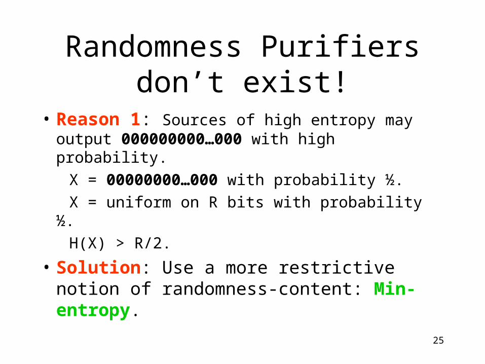
Randomness Purifiers don’t exist!
• Reason 1: Sources of high entropy may output 000000000…000 with high probability.
X = 00000000…000 with probability ½.
X = uniform on R bits with probability ½.
H(X) > R/2.
• Solution: Use a more restrictive notion of randomness-content: Min-entropy.
26
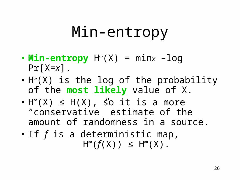
Min-entropy
• Min-entropy H∞(X) = minx –log Pr[X=x].• H∞(X) is the log of the probability of the
most likely value of X.• H∞(X) ≤ H(X), so it is a more
“conservative” estimate of the amount of randomness in a source.
• If f is a deterministic map, H∞(f(X)) ≤ H∞(X).
27
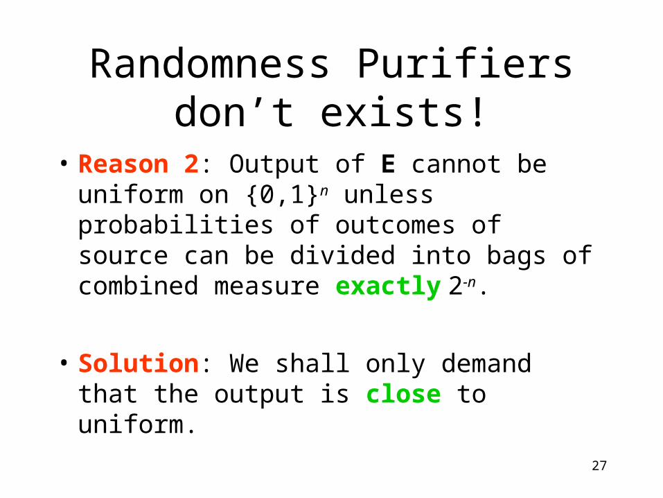
Randomness Purifiers don’t exists!
• Reason 2: Output of E cannot be uniform on {0,1}n unless probabilities of outcomes of source can be divided into bags of combined measure exactly 2-n.
• Solution: We shall only demand that the output is close to uniform.
28
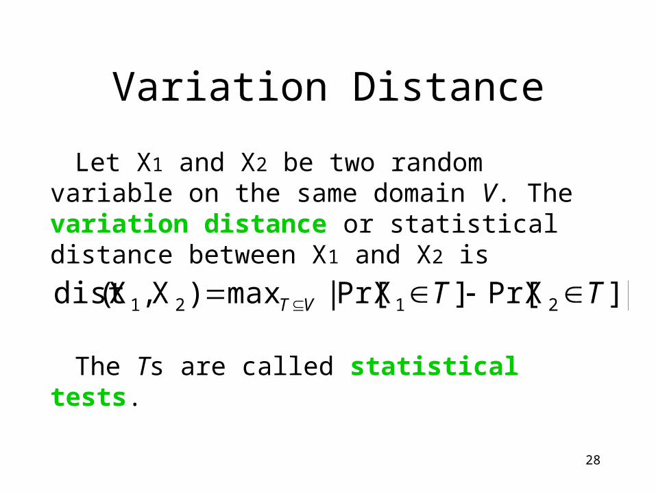
Variation Distance
Let X1 and X2 be two random variable on the same domain V. The variation distance or statistical distance between X1 and X2 is
The Ts are called statistical tests.
|]XPr[]XPr[|max)X,X(dist 2121 TTVT
29
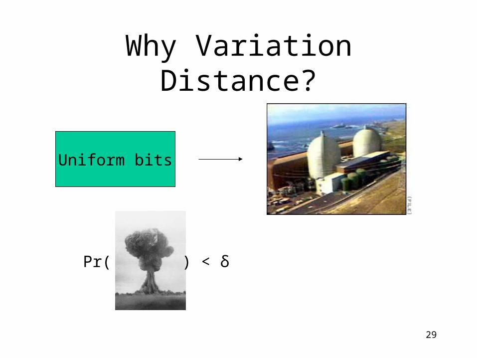
Why Variation Distance?
Uniform bits
Pr( ) < δ
30
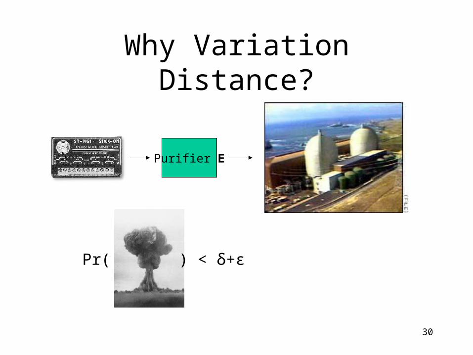
Why Variation Distance?
Pr( ) < δ+ε
Purifier E
31
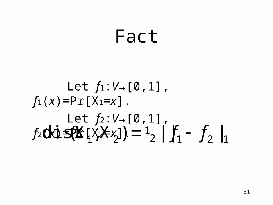
Fact
Let f1:V→[0,1], f1(x)=Pr[X1=x].
Let f2:V→[0,1], f2(x)=Pr[X2=x].
12121
21 ||||)X,X(dist ff
32
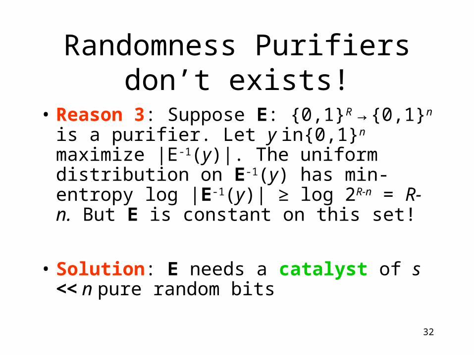
Randomness Purifiers don’t exists!
• Reason 3: Suppose E: {0,1}R → {0,1}n is a purifier. Let y in{0,1}n maximize |E-1(y)|. The uniform distribution on E-1(y) has min-entropy log |E-1(y)| ≥ log 2R-n = R-n. But E is constant on this set!
• Solution: E needs a catalyst of s << n pure random bits
33
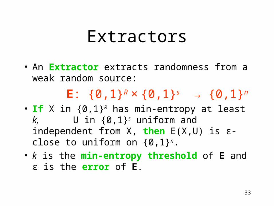
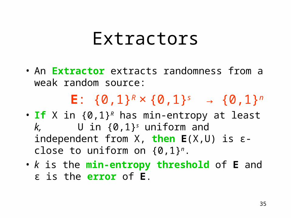
Extractors
• An Extractor extracts randomness from a weak random source:
E: {0,1}R × {0,1}s → {0,1}n
• If X in {0,1}R has min-entropy at least k, U in {0,1}s uniform and independent from X, then E(X,U) is ε-close to uniform on {0,1}n.
• k is the min-entropy threshold of E and ε is the error of E.
34
Fact
• For restricted classes of sources, the pure random bits are not necessary and we may have deterministic extractors.
• Example (Von Neuman): independent, identically distributed random bits.
35
Extractors
• An Extractor extracts randomness from a weak random source:
E: {0,1}R × {0,1}s → {0,1}n
• If X in {0,1}R has min-entropy at least k, U in {0,1}s uniform and independent from X, then E(X,U) is ε-close to uniform on {0,1}n.
• k is the min-entropy threshold of E and ε is the error of E.

36
Dispersers
• A Disperser is an efficient algorithm encoding a particular strategy for finding hay:
D: {0,1}R × {1,..,m} → {0,1}n
• Using R random bits y, the disperser probes T(D(y,1)),…T(D(y,m)).
• The error probability of the disperser is ]0)),(D(:[Prmax
2/1)(, iyTi
yTT
37
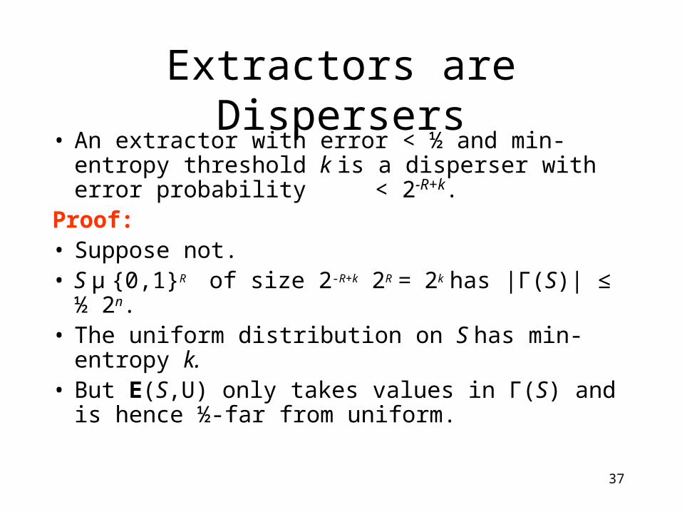
Extractors are Dispersers• An extractor with error < ½ and min-entropy
threshold k is a disperser with error probability < 2-R+k.
Proof:• Suppose not. • S µ {0,1}R of size 2-R+k 2R = 2k has |Γ(S)| ≤ ½ 2n. • The uniform distribution on S has min-entropy k. • But E(S,U) only takes values in Γ(S) and is hence
½-far from uniform.
38
• Extractors have many applications where dispersers cannot be used….
39
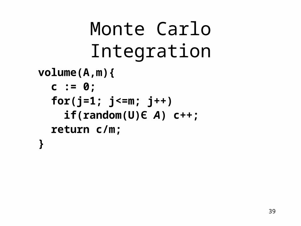
Monte Carlo Integration
volume(A,m){ c := 0; for(j=1; j<=m; j++) if(random(U)Є A) c++; return c/m;}
40
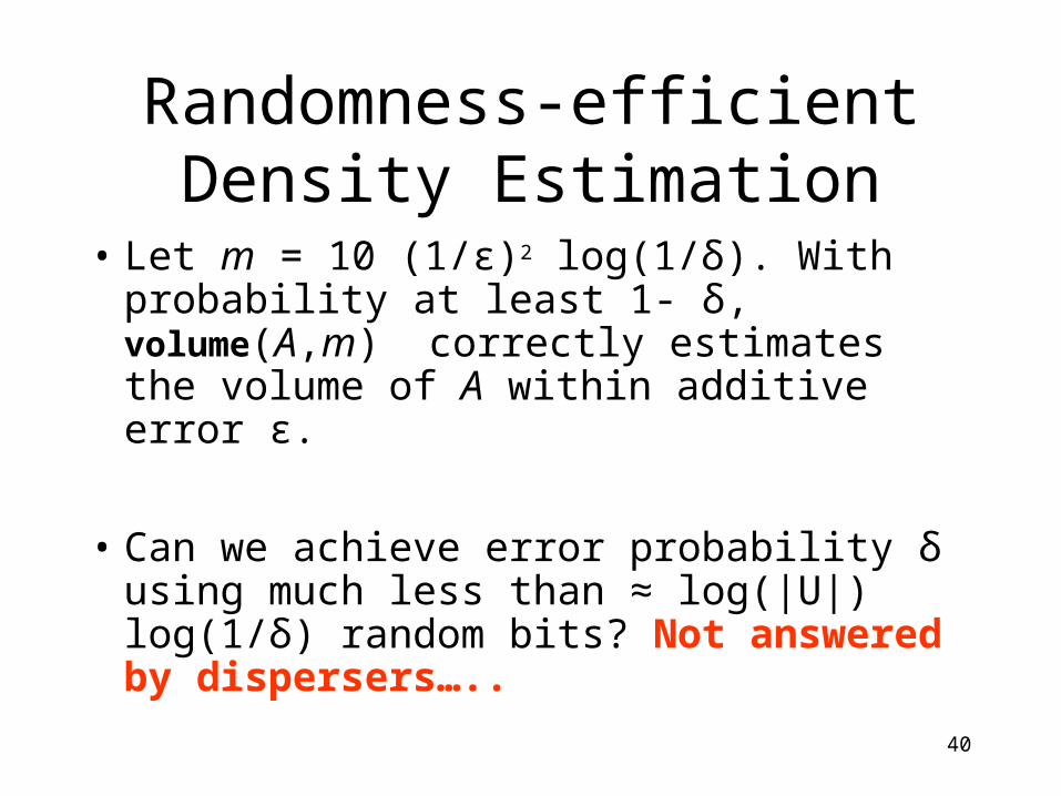
Randomness-efficient Density Estimation
• Let m = 10 (1/ε)2 log(1/δ). With probability at least 1- δ, volume(A,m) correctly estimates the volume of A within additive error ε.
• Can we achieve error probability δ using much less than ≈ log(|U|) log(1/δ) random bits? Not answered by dispersers…..
41
Fact
• An extractor encodes a strategy for randomness-efficient density estimation (fairly easy).
• Conversely, any strategy for randomness efficient density estimation is an extractor (somewhat harder).
• As a consequence, the Chor-Goldreich disperser (pairwise independent random variables) is actually a (weak) extractor.
42
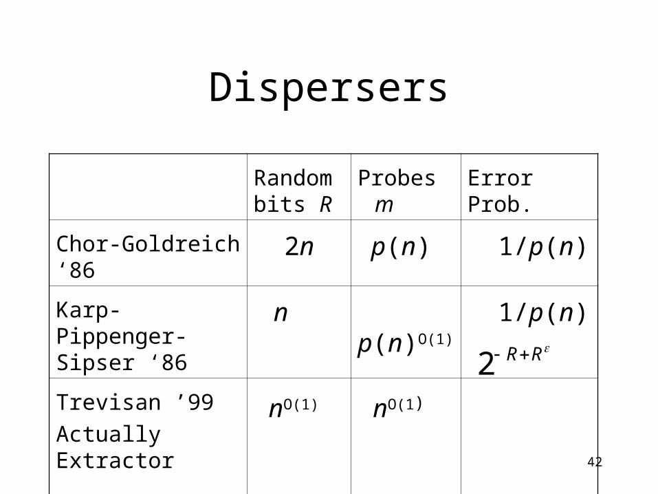
Dispersers
Random bits R
Probes m
Error Prob.
Chor-Goldreich ‘86 2n p(n) 1/p(n)
Karp-Pippenger-Sipser ‘86
n p(n)O(1) 1/p(n)
Trevisan ’99
Actually Extractor
nO(1) nO(1)RR2
43
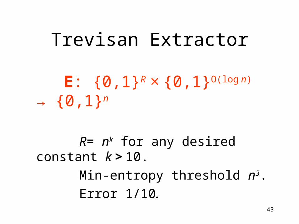
Trevisan Extractor
E: {0,1}R × {0,1}O(log n) → {0,1}n
R= nk for any desired constant k > 10.
Min-entropy threshold n3.
Error 1/10.
44
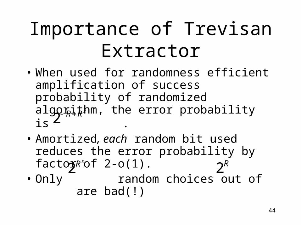
Importance of Trevisan Extractor
• When used for randomness efficient amplification of success probability of randomized algorithm, the error probability is .
• Amortized, each random bit used reduces the error probability by factor of 2-o(1).
• Only random choices out of are bad(!)
RR2
R2 R2
45
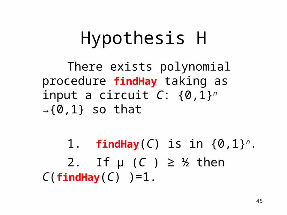
Hypothesis H
There exists polynomial procedure findHay taking as input a circuit C: {0,1}n →{0,1} so that
1. findHay(C) is in {0,1}n.
2. If μ (C ) ≥ ½ then C(findHay(C) )=1.
46
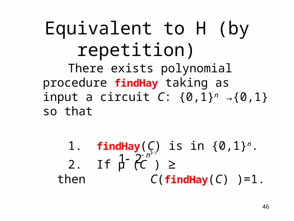
Equivalent to H (by repetition)
There exists polynomial procedure findHay taking as input a circuit C: {0,1}n →{0,1} so that
1. findHay(C) is in {0,1}n.
2. If μ (C ) ≥ then C(findHay(C) )=1.
1
21 n

47
In other words,
It is sufficient to be able to find hay in a haystack of size 2n where the number of needles is at most
1
2 nn
48
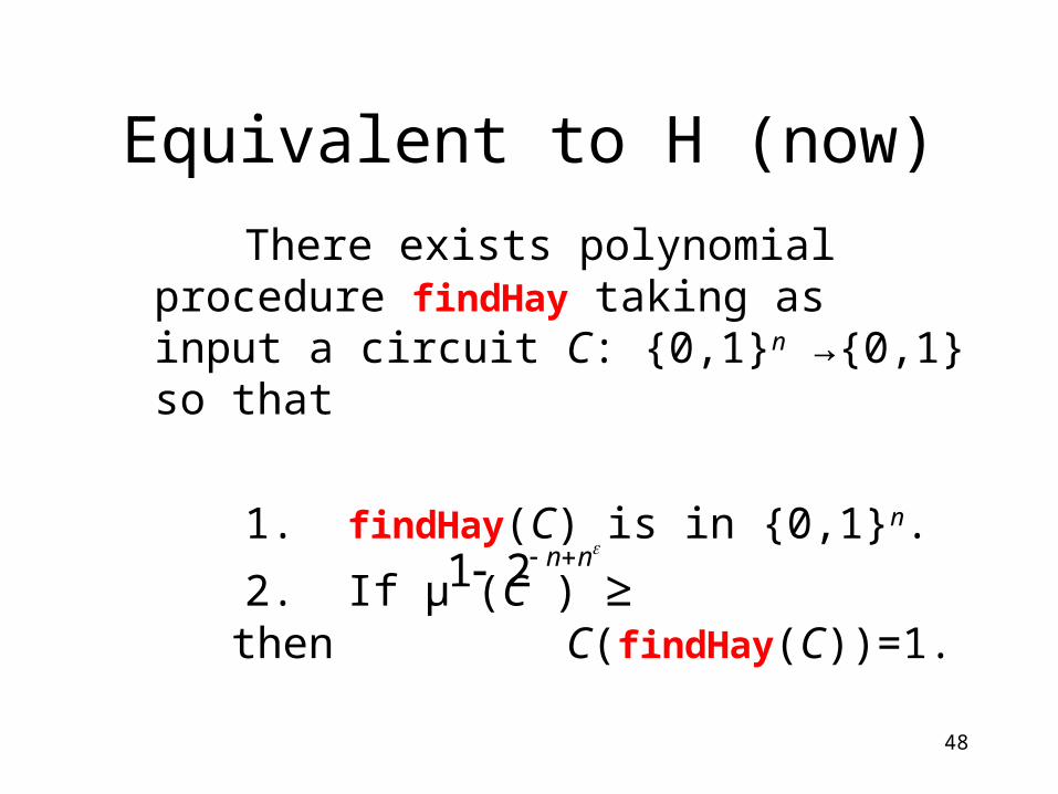
Equivalent to H (now)
There exists polynomial procedure findHay taking as input a circuit C: {0,1}n →{0,1} so that
1. findHay(C) is in {0,1}n.
2. If μ (C ) ≥ then C(findHay(C))=1.
nn 21
49
In other words,
It is sufficient to be able to find hay in a haystack of size 2n where the number of needles is at most
n2
50
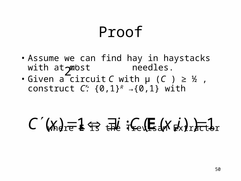
Proof
• Assume we can find hay in haystacks with at most needles.
• Given a circuit C with μ (C ) ≥ ½ , construct C’: {0,1}R →{0,1} with
where E is the Trevisan Extractor
n2
1)),((:1)( ixCixC E
51
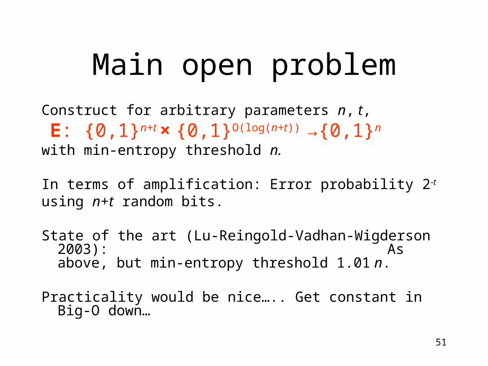
Main open problemConstruct for arbitrary parameters n, t,
E: {0,1}n+t × {0,1}O(log(n+t)) →{0,1}n
with min-entropy threshold n.
In terms of amplification: Error probability 2-t
using n+t random bits.
State of the art (Lu-Reingold-Vadhan-Wigderson 2003): As above, but min-entropy threshold 1.01 n.
Practicality would be nice….. Get constant in Big-O down…
52
Complete derandomization
• To derandomize a randomized algorithm, replace the random bits used by the algorithm by the output of a pseudorandom generator.
• In reality, almost all implemented randomized algorithms have already been derandomized in this way in practice!! So are we wasting our time?
53
The Paradox of Pseudorandomness
54
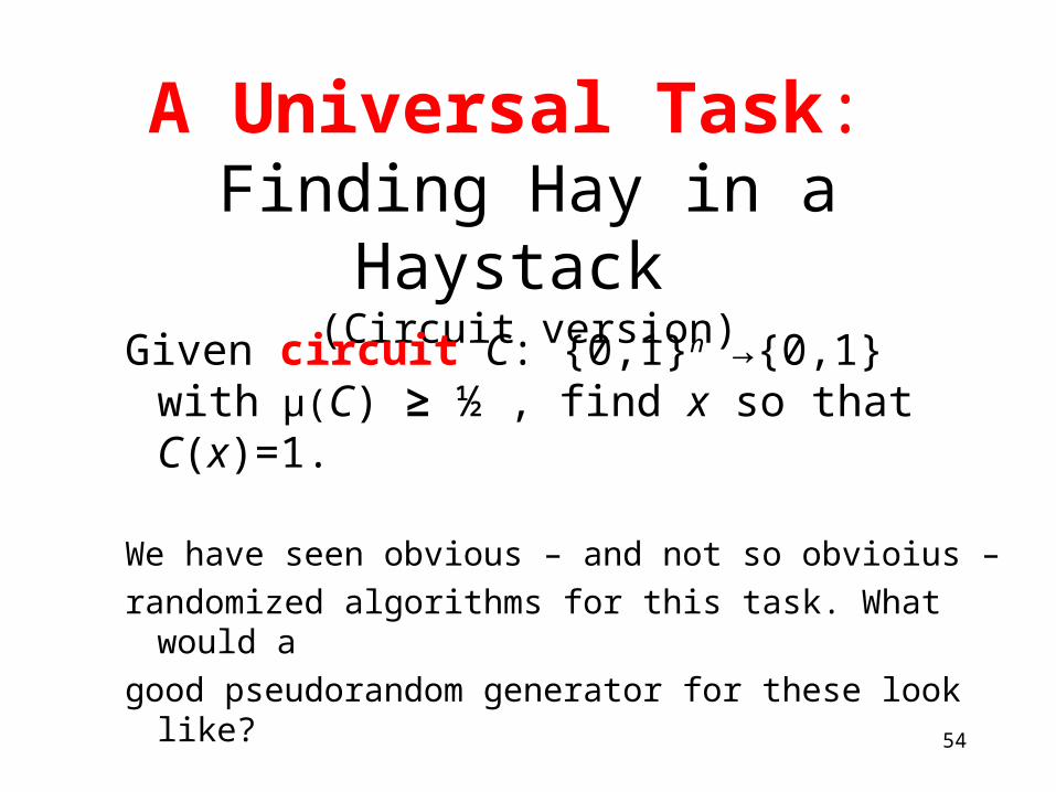
A Universal Task: Finding Hay in a Haystack
(Circuit version)
Given circuit C: {0,1}n →{0,1} with μ(C) ≥ ½ , find x so that C(x)=1.
We have seen obvious – and not so obvioius –
randomized algorithms for this task. What would a
good pseudorandom generator for these look like?
55
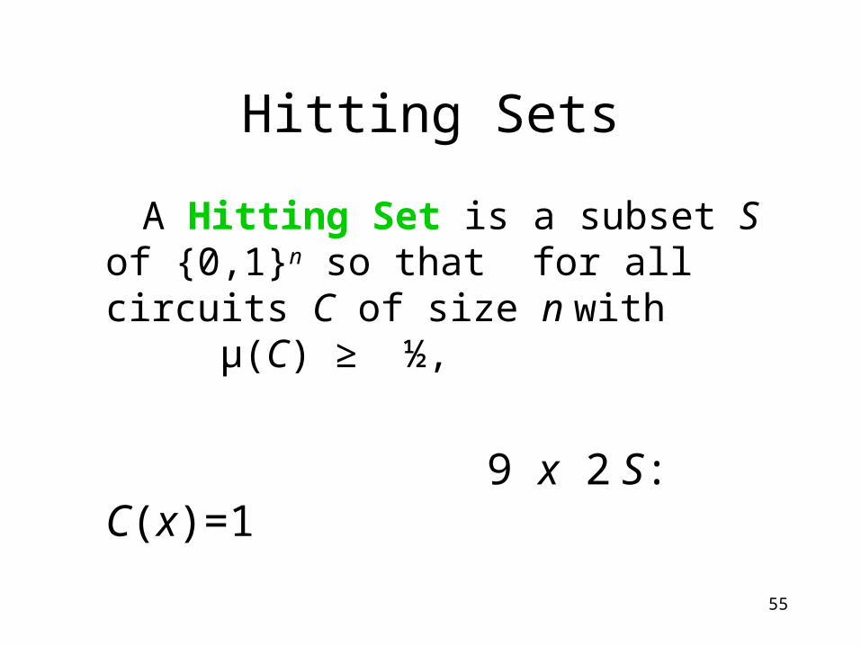
Hitting Sets
A Hitting Set is a subset S of {0,1}n so that for all circuits C of size n with μ(C) ≥ ½,
9 x 2 S: C(x)=1
56
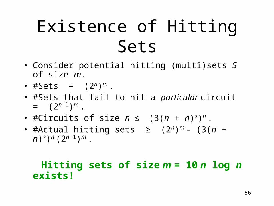
Existence of Hitting Sets
• Consider potential hitting (multi)sets S of size m.• #Sets = (2n)m .• #Sets that fail to hit a particular circuit = (2n-1)m .• #Circuits of size n ≤ (3(n + n)2)n .• #Actual hitting sets ≥ (2n)m - (3(n + n)2)n (2n-1)m .
Hitting sets of size m = 10 n log n exists!
57
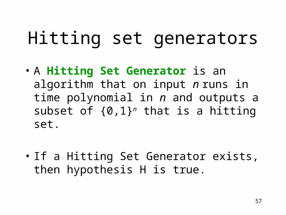
Hitting set generators
• A Hitting Set Generator is an algorithm that on input n runs in time polynomial in n and outputs a subset of {0,1}n that is a hitting set.
• If a Hitting Set Generator exists, then hypothesis H is true.
58
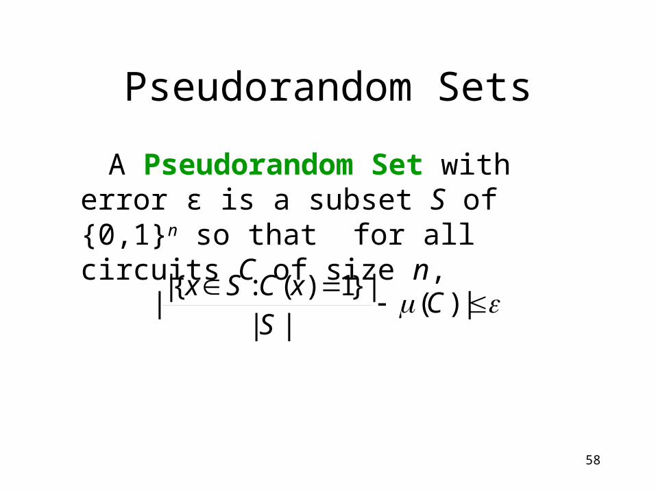
Pseudorandom Sets
A Pseudorandom Set with error ε is a subset S of {0,1}n so that for all circuits C of size n,
|)(
|||}1)(:{|
| CS
xCSx
59
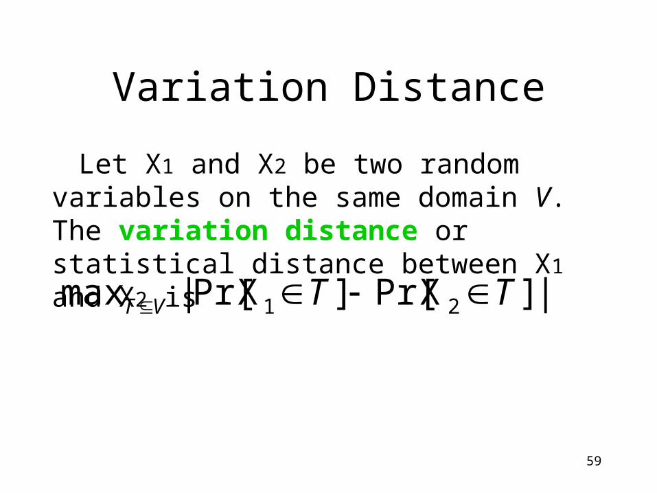
Variation Distance
Let X1 and X2 be two random variables on the same domain V. The variation distance or statistical distance between X1 and X2 is
|]XPr[]XPr[|max 21 TTVT
60
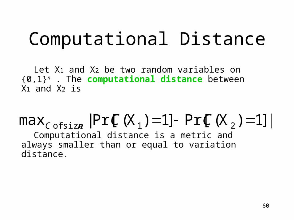
Computational Distance
Let X1 and X2 be two random variables on {0,1}n . The computational distance between X1 and X2 is
Computational distance is a metric and always smaller than or equal to variation distance.
|]1)X(Pr[]1)X(Pr[|max 21 size of CCnC
61
Pseudorandom Sets, Alternative Definition
A Pseudorandom Set with error ε is a subset S of {0,1}n so that the uniform distribution on S is ε-close to uniform in computational distance.
62
Pseudorandom Generators
• A Pseudorandom Generator is an algorithm that on input n runs in time polynomial in n and outputs a subset of {0,1}n that is a pseudorandom set.
• Pseudorandom sets are also hitting sets, so pseudorandom generators are also hitting set generators.
• A Pseudorandom Generator can be used to directly derandomize Monte Carlo density estimation.
63
PRGs vs. Crypto-PRGs
• Our generators don’t use seeds!
• We know the exact computational power of our adversary in advance and can use more time than he.
• What is a good candidate for our kind of generator?
64
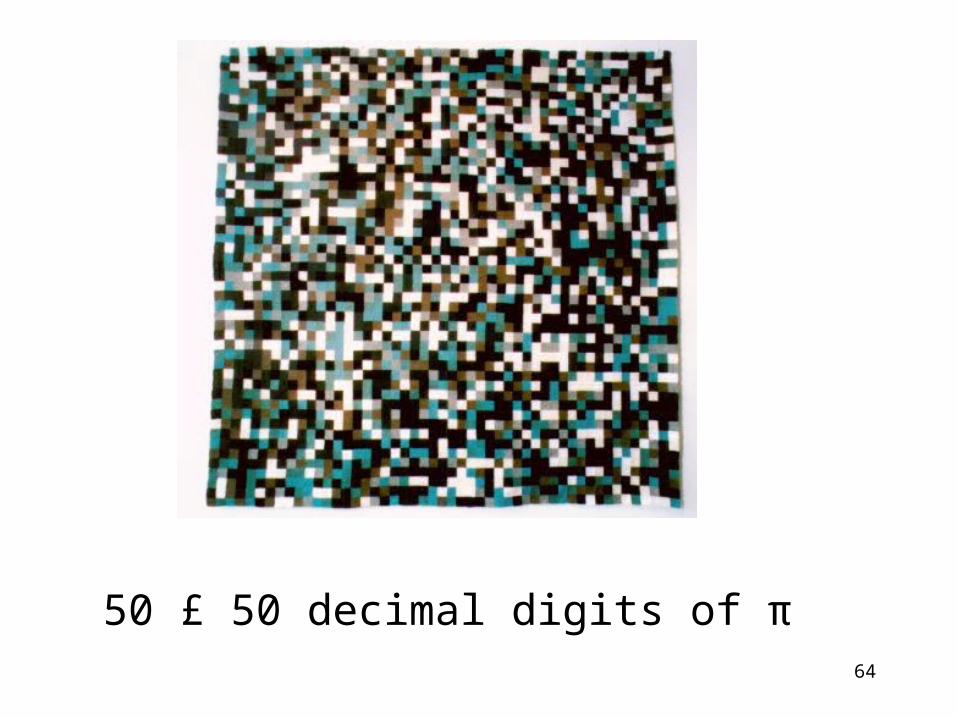
50 £ 50 decimal digits of π
65
66
67
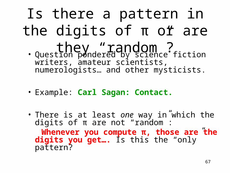
Is there a pattern in the digits of π or are they “random”?
• Question pondered by science fiction writers, amateur scientists, numerologists… and other mysticists.
• Example: Carl Sagan: Contact.
• There is at least one way in which the digits of π are not “random”:
Whenever you compute π, those are the digits you get…. Is this the “only” pattern?
68
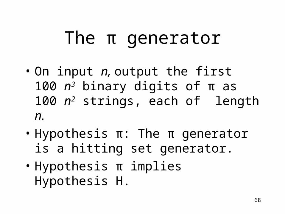
The π generator
• On input n, output the first 100 n3 binary digits of π as 100 n2 strings, each of length n.
• Hypothesis π: The π generator is a hitting set generator.
• Hypothesis π implies Hypothesis H.
69
A Win-Win Situation
• From now on, I’m going to assume Hypothesis π and always use the π generator to find hay.
• Case 1: I’ll never run into any problems. GREAT!
• Case 2: One day we fail to find hay in a haystack, so the π generator is not a hitting set generator after all. STILL GREAT(!)
70
Why is this still great?
• Suppose the generator fails, say, for n=100.
• I have found a simple property (described by a circuit of size 100) that is satisfied by half of all 100-bit strings but which none of the first 1000000 blocks of 100 bits of π satisfies.
• AMAZING! This is what all the amateur scientists were looking for and much more convincing than the “patterns” they found.

71
72
Philosophical interpretation
• Hypothesis π is just one way in which we may establish Hypothesis H.
• If Hypothesis H is false, there are amazing patterns to be found everywhere – not just in π. How great!
• Thus I tend to think H is true……
73
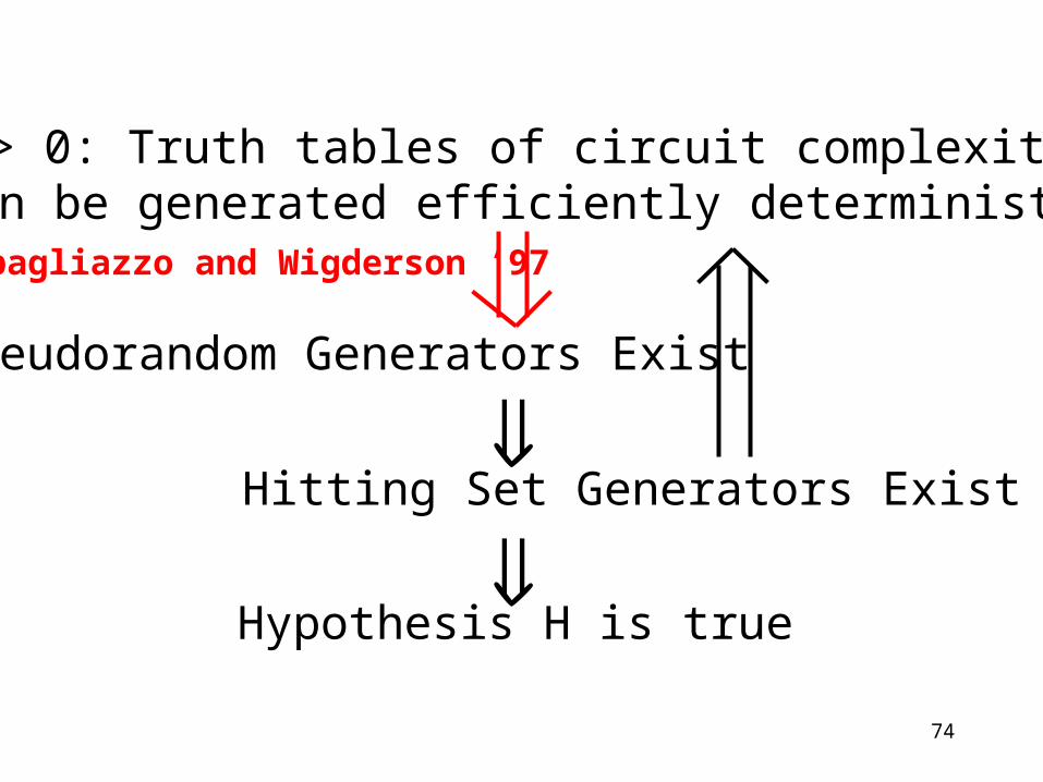
Hitting set generators derandomize the construction of hard truth tables
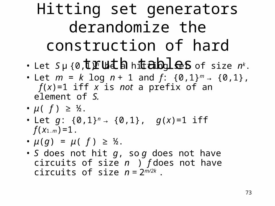
• Let S µ {0,1}n be a hitting set of size nk. • Let m = k log n + 1 and f: {0,1}m → {0,1}, f(x)=1
iff x is not a prefix of an element of S.• μ( f ) ≥ ½.• Let g: {0,1}n → {0,1}, g(x)=1 iff f(x1.m)=1.• μ(g) = μ( f ) ≥ ½.• S does not hit g, so g does not have circuits of size
n ) f does not have circuits of size n = 2m/2k .
74
Hitting Set Generators Exist
Hypothesis H is true
9 ε > 0: Truth tables of circuit complexity >2εn can be generated efficiently deterministically.
Pseudorandom Generators Exist
Impagliazzo and Wigderson ‘97
75
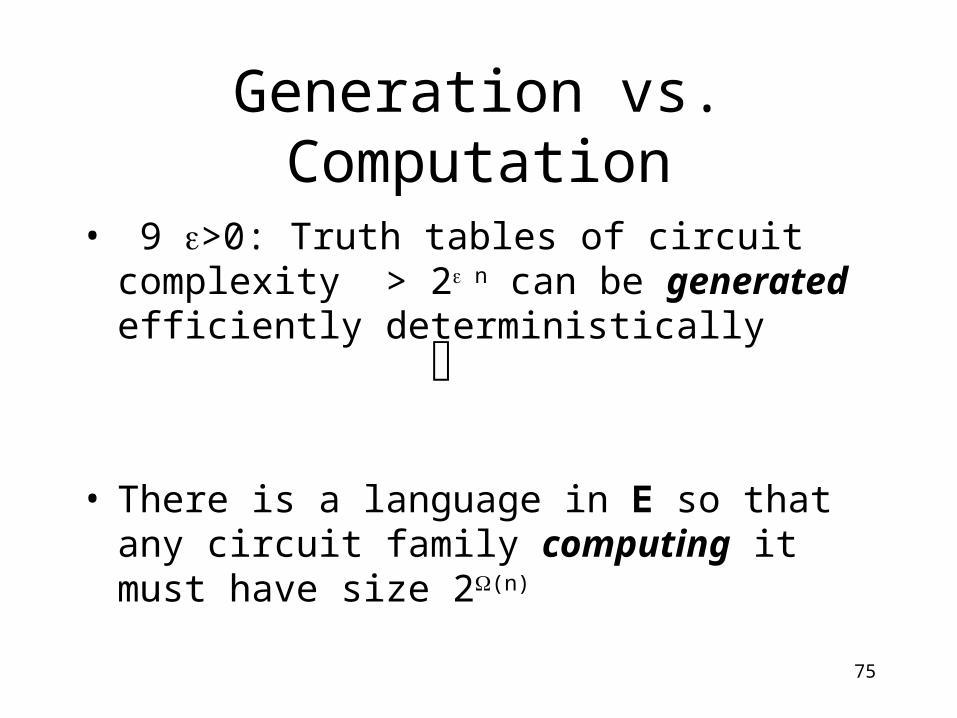
Generation vs. Computation
• 9 >0: Truth tables of circuit complexity > 2 n can be generated efficiently deterministically
• There is a language in E so that any circuit family computing it must have size 2(n)
⇕
76
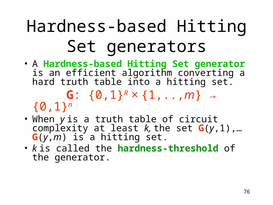
Hardness-based Hitting Set generators
• A Hardness-based Hitting Set generator is an efficient algorithm converting a hard truth table into a hitting set.
G: {0,1}R × {1,..,m} → {0,1}n
• When y is a truth table of circuit complexity at least k, the set G(y,1),…G(y,m) is a hitting set.
• k is called the hardness-threshold of the generator.

77
Dispersers
• A Disperser is an efficient algorithm encoding a particular strategy for finding hay:
D: {0,1}R × {1,..,m} → {0,1}n
• Using R random bits y, the disperser probes T(D(y,1)),…T(D(y,m)).
• The error probability of the disperser is ]0)),(D(:[Prmax
2/1)(, iyTi
yTT
78
• Hardness-based hitting set generators are dispersers.
• Hardness-based pseudorandom generators are extractors.
79
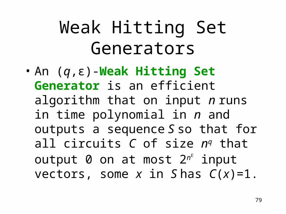
Weak Hitting Set Generators
• An (q,ε)-Weak Hitting Set Generator is an efficient algorithm that on input n runs in time polynomial in n and outputs a sequence S so that for all circuits C of size nq that output 0 on at most 2n input vectors, some x in S has C(x)=1.
80
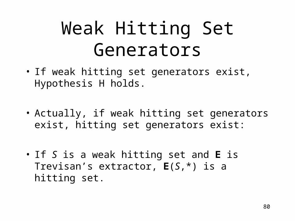
Weak Hitting Set Generators
• If weak hitting set generators exist, Hypothesis H holds.
• Actually, if weak hitting set generators exist, hitting set generators exist:
• If S is a weak hitting set and E is Trevisan’s extractor, E(S,*) is a hitting set.
81
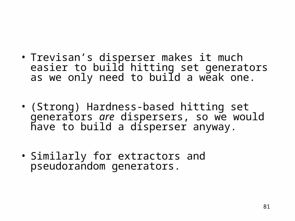
• Trevisan’s disperser makes it much easier to build hitting set generators as we only need to build a weak one.
• (Strong) Hardness-based hitting set generators are dispersers, so we would have to build a disperser anyway.
• Similarly for extractors and pseudorandom generators.

82
Incompressibility of computation
9 k>0 and a deterministic algorithm A running in time t = 2kn so that any algorithm using spacet0.999 fails to simulate A on all sufficiently largeinput lengths.
Hypothesis H is true
83
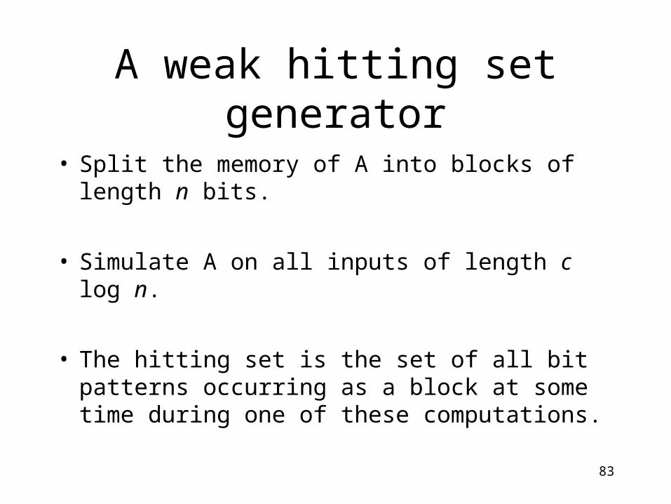
A weak hitting set generator
• Split the memory of A into blocks of length n bits.
• Simulate A on all inputs of length c log n.
• The hitting set is the set of all bit patterns occurring as a block at some time during one of these computations.

84
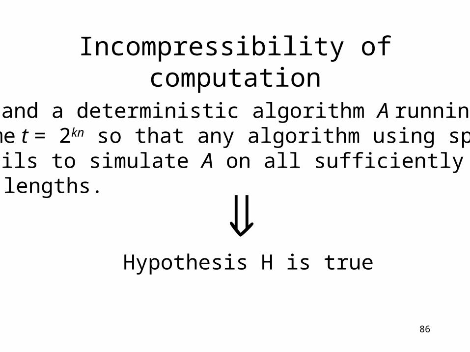
Incompressibility of computation
9 k>0 and a deterministic algorithm A running in time t = 2kn so that any algorithm using spacet0.999 fails to simulate A on all sufficiently largeinput lengths.
Hypothesis H is true
85
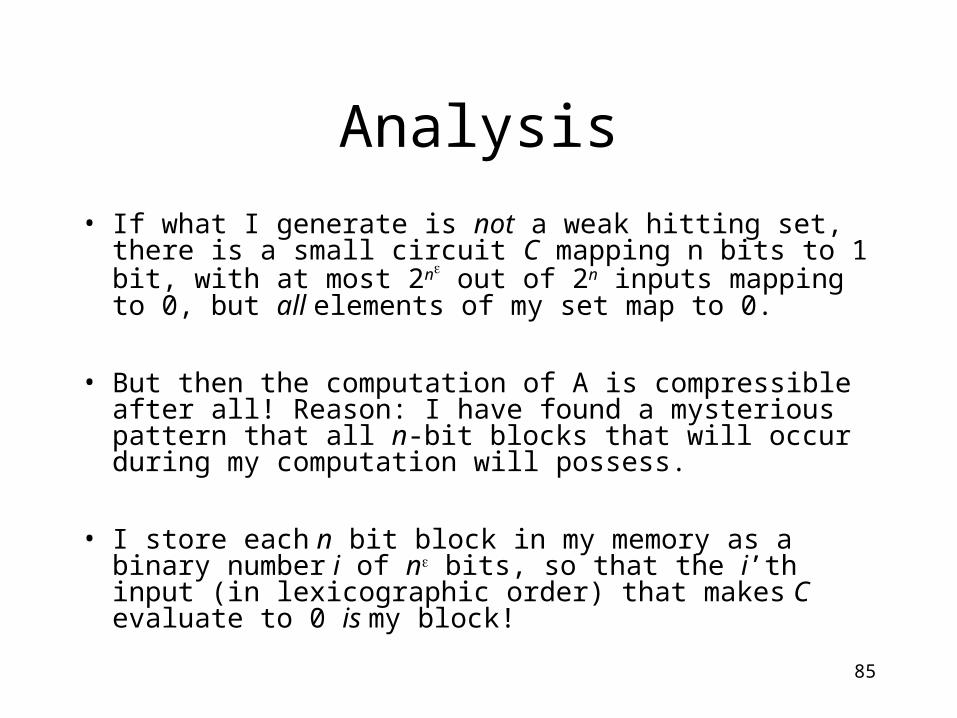
Analysis
• If what I generate is not a weak hitting set, there is a small circuit C mapping n bits to 1 bit, with at most 2n out of 2n inputs mapping to 0, but all elements of my set map to 0.
• But then the computation of A is compressible after all! Reason: I have found a mysterious pattern that all n-bit blocks that will occur during my computation will possess.
• I store each n bit block in my memory as a binary number i of n bits, so that the i’th input (in lexicographic order) that makes C evaluate to 0 is my block!
86
Incompressibility of computation
9 k>0 and a deterministic algorithm A running in time t = 2kn so that any algorithm using spacet0.999 fails to simulate A on all sufficiently largeinput lengths.
Hypothesis H is true
87
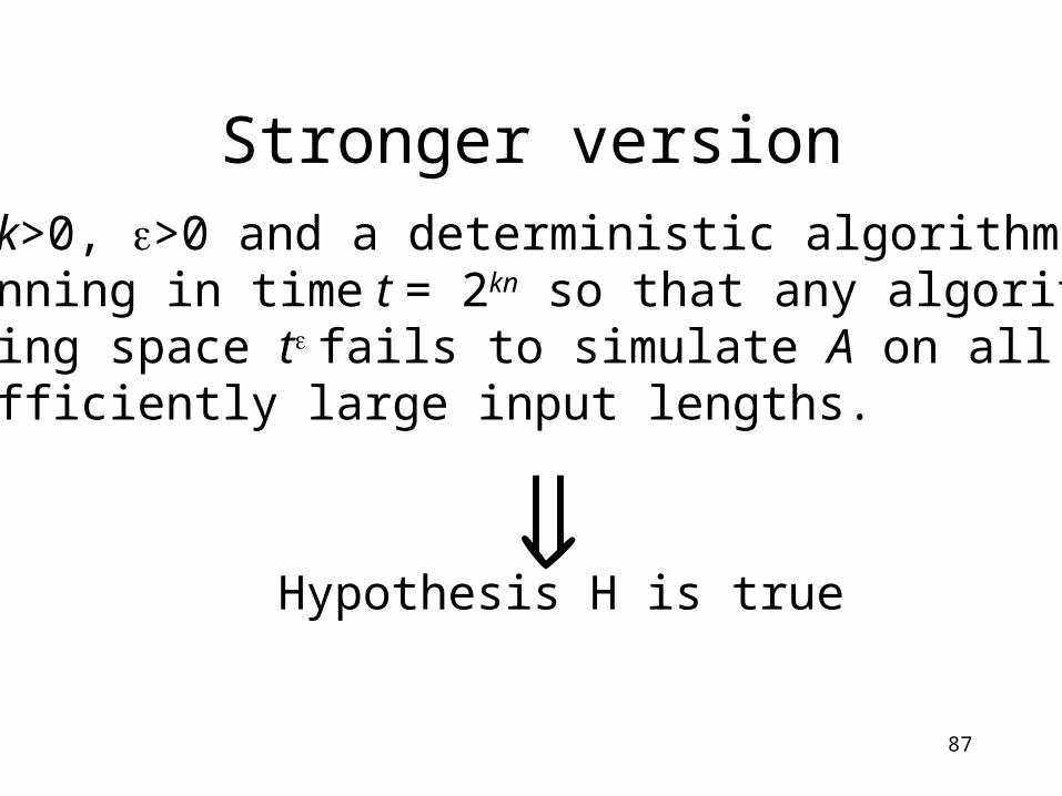
Stronger version9 k>0, >0 and a deterministic algorithm A running in time t = 2kn so that any algorithm using space t fails to simulate A on all sufficiently large input lengths.
Hypothesis H is true
88
Disclaimer
• These lectures have focused mainly on definitions and have barely scratched the surface of the field of derandomization.
![C´alculo estoc´astico - UM¥ La funci«on F X: R % [0,1] es creciente, continua por la derecha y con lõmit« es iguales a cero en (- y1en+- . ¥ Si la variable X tiene densidad](https://static.fdocument.org/doc/165x107/5edc987fad6a402d6667539d/calculo-estocastico-um-la-funcion-f-x-r-01-es-creciente-continua.jpg)
![1 Appendix: Common distributionsfaculty.chicagobooth.edu/nicholas.polson/teaching/41900/Appendices...1 Appendix: Common distributions ... Beta • A random variable X ∈ [0,1] has](https://static.fdocument.org/doc/165x107/5ae3e1407f8b9a595d8f03f5/1-appendix-common-appendix-common-distributions-beta-a-random-variable.jpg)