010 141010.141 MODULE 2: Matrix Eigenvalue...

ENGINEERING MATHEMATICS IIENGINEERING MATHEMATICS II

010 141010.141

MODULE 2: Matrix Eigenvalue ProblemProblem

EIGENVALUES AND EIGENVECTORSEIGENVALUES AND EIGENVECTORS

2B.D. Youn2010 Engineering Mathematics II Module 2

SOME DEFINITIONS

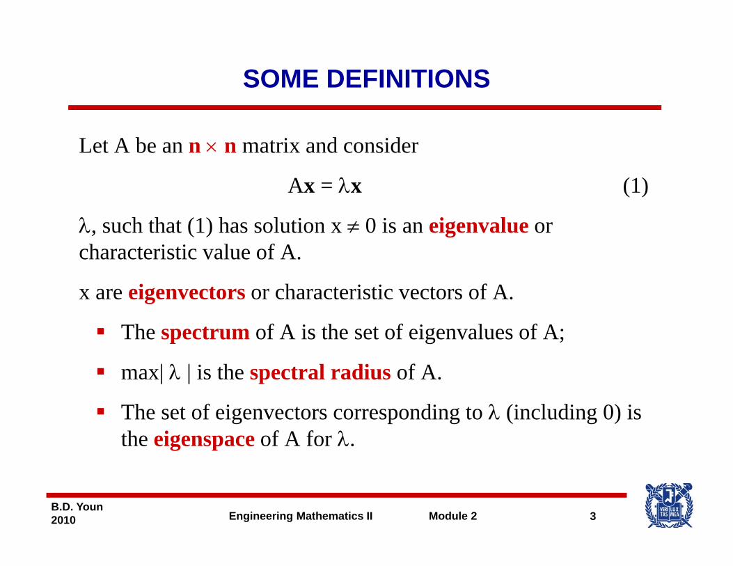
Let A be an n × n matrix and consider

Ax = λx (1)

λ, such that (1) has solution x ≠ 0 is an eigenvalue or h t i ti l f Acharacteristic value of A.

x are eigenvectors or characteristic vectors of A.

The spectrum of A is the set of eigenvalues of A;

max| λ | is the spectral radius of A.

The set of eigenvectors corresponding to λ (including 0) is the eigenspace of A for λ.


SOME DEFINITIONS (cont)

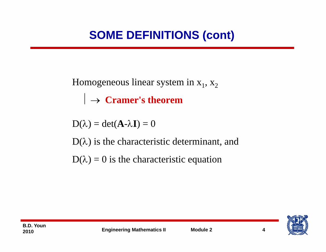
li iHomogeneous linear system in x1, x2

⏐→ Cramer's theorem

D(λ) = det(A-λI) = 0

D(λ) is the characteristic determinant andD(λ) is the characteristic determinant, and

D(λ) = 0 is the characteristic equation


DETERMINATION OF EIGENVALUES AND EIGENVECTORS

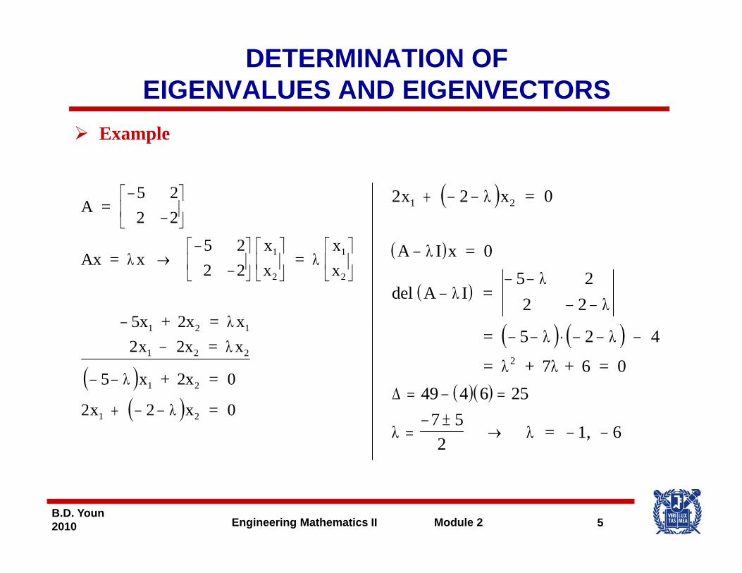
Example

A

x x

= 5

2

5

−−

⎡

⎣⎢

⎤

⎦⎥

−⎡ ⎤ ⎡ ⎤ ⎡ ⎤

22

2 1 1

( )

( )

2 0x 2 x =

A = 0

1 2+ − − λ

λ I xAx xx

xx= x

5 2 =

5x + 2x = x

→−

⎡

⎣⎢

⎤

⎦⎥⎡

⎣⎢

⎤

⎦⎥

⎡

⎣⎢

⎤

⎦⎥

−

22

1

2

1

2λ λ

λ

( )

( )2

2

A = 0

del A = 5

2

−

−− −

− −

λ

λλ

λ

I x

I

( )

5x + 2x = x x 2x = x

5 x + 2x =

1 2 1

1 2 2

1 2

−−

− −

2

0

λλ

λ

( ) ( )

( )( )

2

49 4 6 25

= 5 4

= + 7 + 6 = 02

− − ⋅ − − −

= − =

λ λ

λ λ

Δ( )x 2 x = 1 2+ − −2 0λ

( )( )49 4 6 257 52

= 1, 6

= − =

=− ±

→ − −λ λ

Δ


DETERMINATION OF EIGENVALUES AND EIGENVECTORS (cont)Eigenvector for λ = -1

( )( )

− + + =+ − + =

5 x 2x x x

4 2

1 2

1 2

1 02 2 1 0

0− + =− =

4x 2x x x

2 +

1 2

1 2

02 0

0− =

=

2x + x

xx

1 2

12

0

2⎛⎝⎜

⎞⎠⎟

21 21


DETERMINATION OF EIGENVALUES AND EIGENVECTORS (cont)

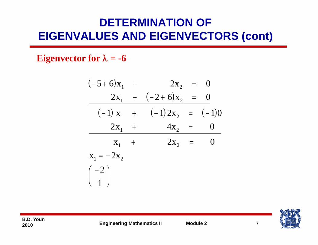
Eigenvector for λ = -6

( )( )

− + + =+ − + =

5 x 2x x x

1 2

1 2

6 02 2 6 0

( ) ( ) ( )− + − = −+ =

x 2x x 4x

1 2

1 2

1 1 1 02 0

+ == −

⎛ ⎞

x 2xx 2x

1 2

1 2

0

2−⎛⎝⎜

⎞⎠⎟

21


EIGENVALUES

The eigenvalues of a square matrix A are the roots of theThe eigenvalues of a square matrix A are the roots of the characteristic equation

D(λ) = 0

An n × n matrix has at least one eigenvalue and at most n different eigenvaluesn different eigenvalues


EIGENVECTORS

If x is an eigenvector of a matrix A corresponding to anIf x is an eigenvector of a matrix A corresponding to an eigenvalue λ, so is kx with any k ≠ 0.

P fProof:Ax = λx

k(Ax) = kλxk(Ax) kλxA(kx) = λ(kx)


PROBLEM

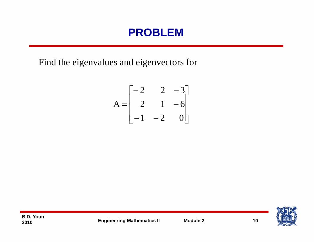
Find the eigenvalues and eigenvectors for

⎥⎥⎤

⎢⎢⎡

−−−

= 61232 2

A⎥⎥⎦⎢

⎢⎣ −− 0 21

61 2 A


MULTIPLICITY

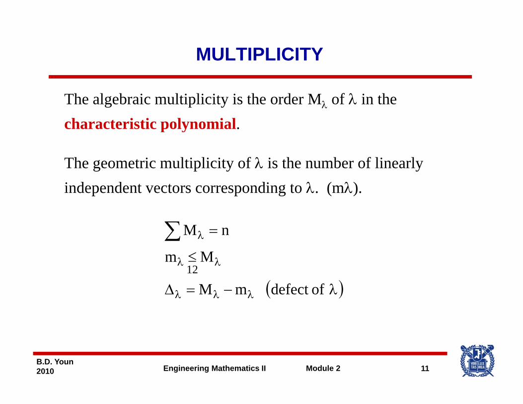
The algebraic multiplicity is the order Mλ of λ in the characteristic polynomialcharacteristic polynomial.

The geometric multiplicity of λ is the number of linearly independent vectors corresponding to λ. (mλ).

∑M

≤

=

λλ

λ∑Mm

nM

12

( )λ−=Δ λλλ ofdefect mM


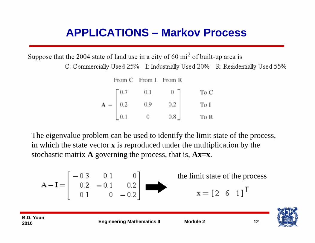
APPLICATIONS – Markov Process

The eigenvalue problem can be used to identify the limit state of the processThe eigenvalue problem can be used to identify the limit state of the process, in which the state vector x is reproduced under the multiplication by the stochastic matrix A governing the process, that is, Ax=x.

the limit state of the process


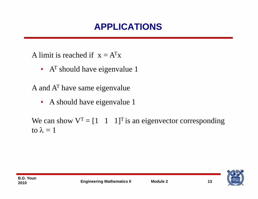
APPLICATIONS

A limit is reached if x = ATx

• AT should have eigenvalue 1

A and AT have same eigenvalueA and AT have same eigenvalue

• A should have eigenvalue 1

We can show VT = [1 1 1]T is an eigenvector corresponding to λ = 1


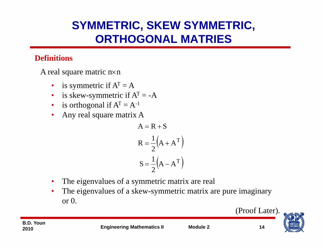
SYMMETRIC, SKEW SYMMETRIC, ORTHOGONAL MATRIES

Definitions

A real square matric n×n

• is symmetric if AT = A• is skew-symmetric if AT = -A• is orthogonal if AT = A-1g• Any real square matrix A

( )TAA1SRA +=

( )( )T

T

AA21S

AA21R

−=

+=

• The eigenvalues of a symmetric matrix are real• The eigenvalues of a skew-symmetric matrix are pure imaginary

or 0.

2


or 0.(Proof Later).

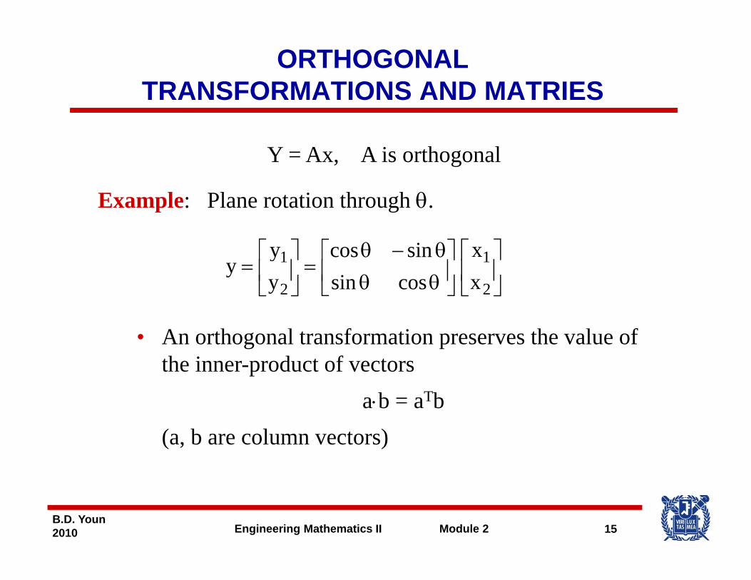
ORTHOGONALTRANSFORMATIONS AND MATRIES

Y = Ax, A is orthogonal

Example: Plane rotation through θ.

⎤⎡⎤⎡ θ−θ⎤⎡ 11 xsincosy⎥⎦

⎤⎢⎣

⎡⎥⎦

⎤⎢⎣

⎡θθθθ

=⎥⎦

⎤⎢⎣

⎡=

2

1

2

1

xx

cossinsincos

yy

y

• An orthogonal transformation preserves the value of the inner-product of vectors

a b = aTba⋅b = aTb(a, b are column vectors)


ORTHOGONALTRANSFORMATIONS AND MATRIES (cont)

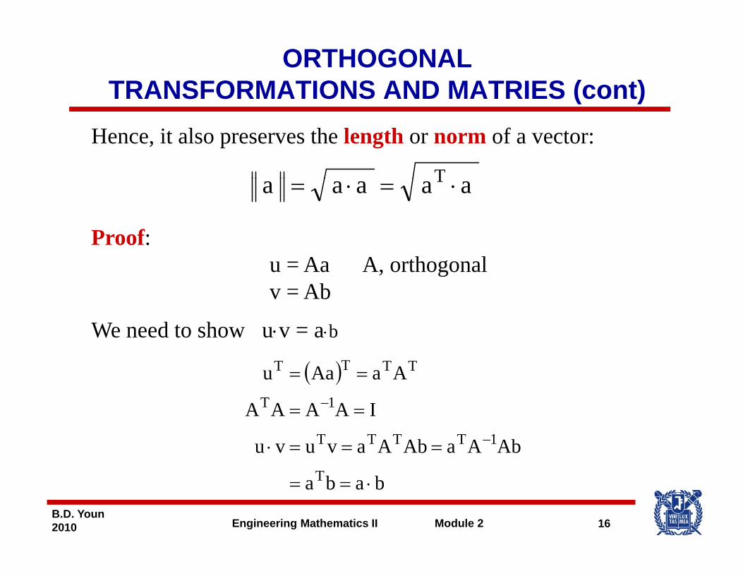
Hence, it also preserves the length or norm of a vector:

T

Proof:

aaaaa T ⋅=⋅=

u = Aa A, orthogonalv = Ab

W d hWe need to show u⋅v = a⋅b

( ) AaAau TTTT ==

AbAaAbAavuvu

IAAAA1TTTT

1T

===⋅

==−

−


babaT ⋅==

ORTHONORMALITY OFCOLUMN AND ROW VECTORS

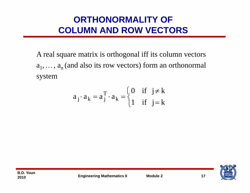
A real square matrix is orthogonal iff its column vectors a1, …, an (and also its row vectors) form an orthonormal system

⎩⎨⎧

=≠

=⋅=⋅k j if1k j if0

aaaa kTjkj


ORTHONORMALITY OFCOLUMN AND ROW VECTORS

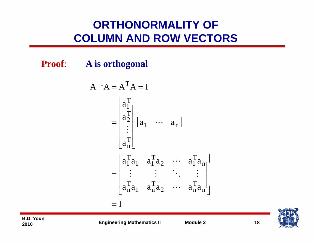
Proof: A is orthogonal

a

IAAAAT1

T1

⎥⎤

⎢⎡

==−

[ ]aaan1

T

T2

1

⎥⎥⎥⎥

⎢⎢⎢⎢

=

aaaaaa

a

nT12

T11

T1

Tn

⎥⎤

⎢⎡

⎥⎥⎦⎢

⎢⎣

aaaaaa nTn2

Tn1

Tn

⎥⎥⎥

⎦⎢⎢⎢

⎣

=


I=

DETERMINANT OF AN ORTHOGONAL MATRIX

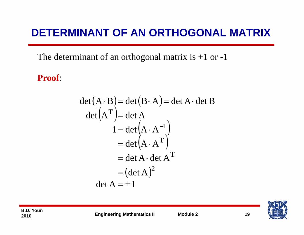
The determinant of an orthogonal matrix is +1 or -1

Proof:

( ) ( ) BdetAdetABdetBAdet ⋅=⋅=⋅( ) ( )( )

( )AAdet1AdetAdet

BdetAdetABdetBAdet

1

T

⋅==

−( )( )

AdetAdetAAdetAAdet1

T

T

⋅=⋅=

( )1Adet

Adet 2

±==


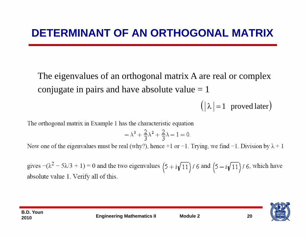
DETERMINANT OF AN ORTHOGONAL MATRIX

Th i l f th l t i A l lThe eigenvalues of an orthogonal matrix A are real or complex conjugate in pairs and have absolute value = 1

( )ld1λ( )laterproved 1=λ


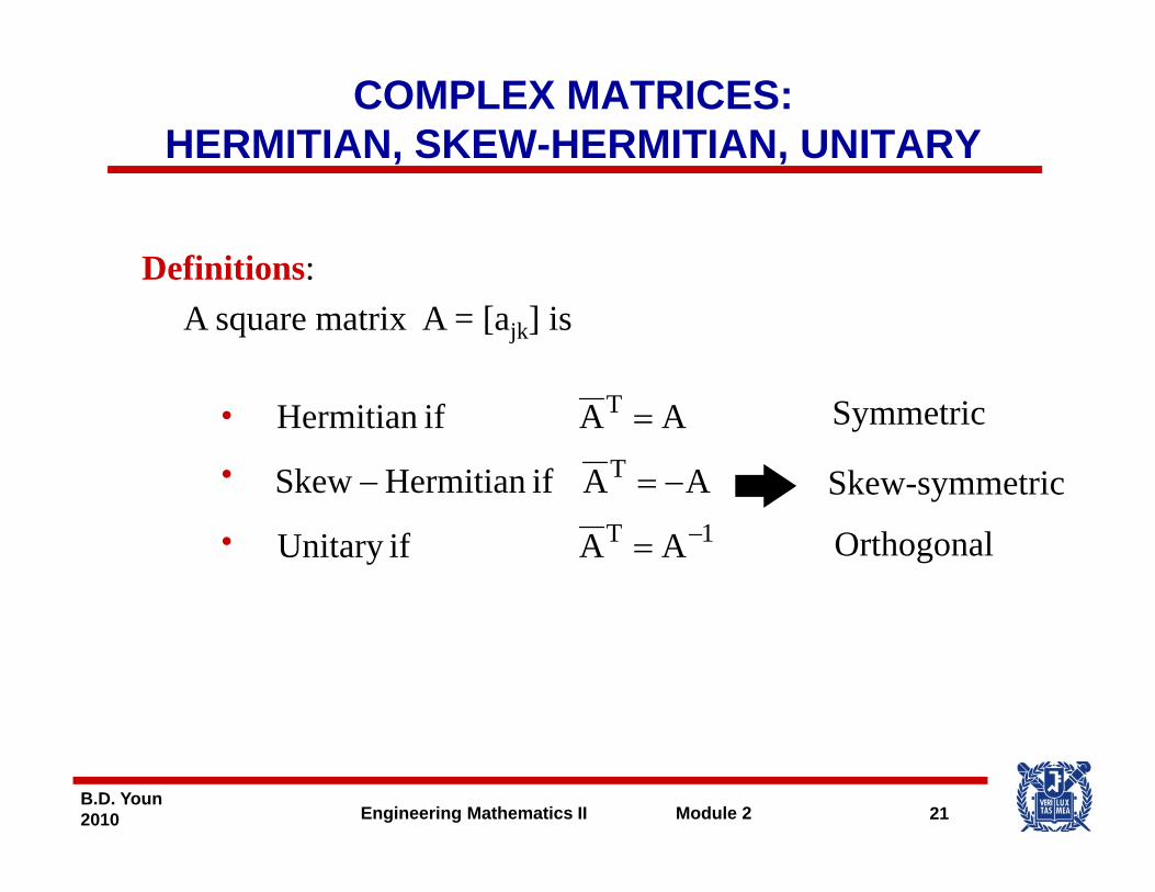
COMPLEX MATRICES: HERMITIAN, SKEW-HERMITIAN, UNITARY

Definitions:Definitions:A square matrix A = [ajk] is

•

• T

T

AA if HermitianSkew

AA if Hermitian

−=−

= Symmetric

Skew-symmetric

• 1T AA if Unitary −= Orthogonal


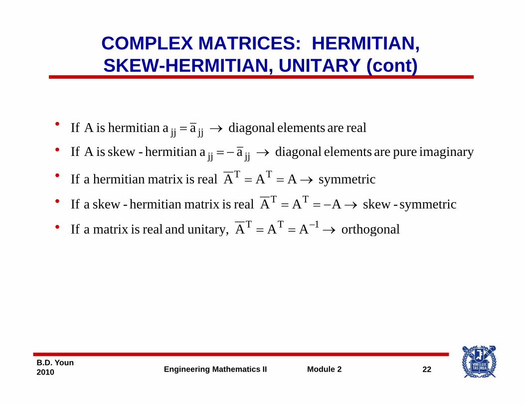
COMPLEX MATRICES: HERMITIAN, SKEW-HERMITIAN, UNITARY (cont)

•

( )

realareelementsdiagonalaaermitianhisAIf →

•• t iAAAlit ih itiIf

imaginary pure are elements diagonal a a hermitianskew isA If

realare elementsdiagonal aa ermitianh isA If

TT

jjjj

jjjj

→

→−=

→=

••• orthogonalAAAnitaryuandrealismatrixaIf

symmetric-skew AAA real ismatrix hermitian-skew a If

symmetric AAA realismatrix hermitian a If

1TT

TT

TT

→

→−==

→==

−• orthogonal AAA ,nitaryuand real ismatrix a If →==


EIGENVALUES

Theorem:

• The eigenvalues of a Hermitian matrix are real.

• The eigenvalues of a skew Hermitian matrix are• The eigenvalues of a skew-Hermitian matrix are pure imaginary or 0.

• The eigenvalues of a unitary matrix have absoluteThe eigenvalues of a unitary matrix have absolute value of "1".


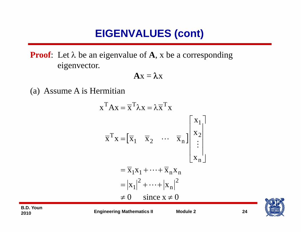
EIGENVALUES (cont)

Proof: Let λ be an eigenvalue of A, x be a corresponding eigenvector.

Ax = λx

(a) Assume A is Hermitian

xxxxxAxx

1

TTT

⎥⎤

⎢⎡

λ=λ=

[ ]

x

xxxxxx

n

2n21

T

⎥⎥⎥⎥

⎦⎢⎢⎢⎢

⎣

=

xx

xxxx2

n2

1

nn11

n

++=

++=⎦⎣


0x since 0 ≠≠

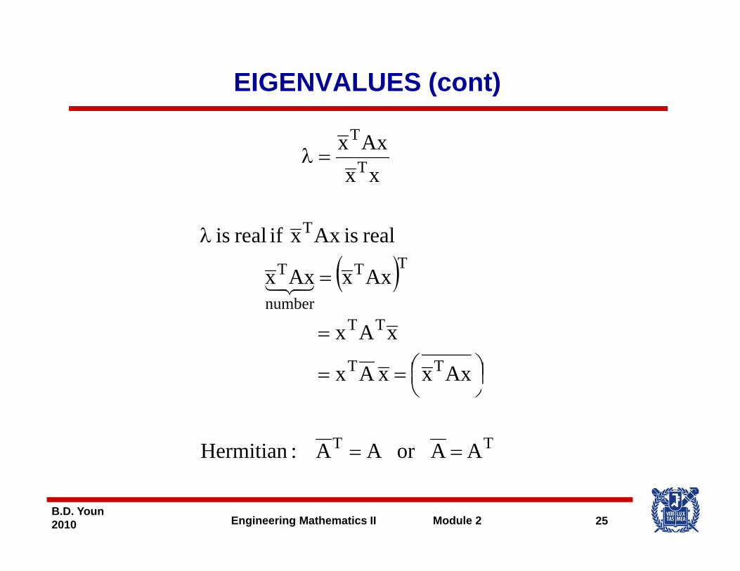
EIGENVALUES (cont)

T

T

xxAxx =λ

T real is Axx if real is

xx

λ

( )TT

TT

number

T AxxAxx =

TT

TT

AxxxAx

xAx

⎟⎠⎞⎜

⎝⎛==

=

TT A Aor AA :Hermitian ==

⎠⎝


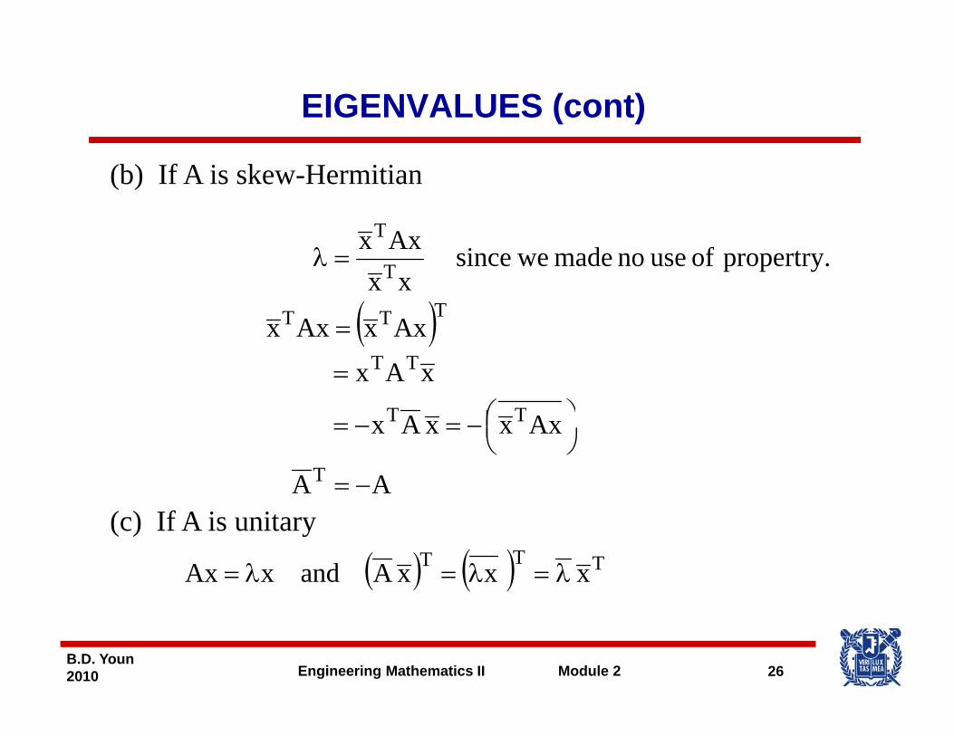
EIGENVALUES (cont)

T

(b) If A is skew-Hermitian

( )TTT

T

T

AA

propertry. of use no made wesince xx

Axx =λ

( )

TT

TT

TT

xAx

AxxAxx

⎟⎞⎜⎛

=

=

T

TT

AA

AxxxAx

−=

⎟⎠⎞⎜

⎝⎛−=−=

( ) ( ) TTT x xxA and xAx λ=λ=λ=

(c) If A is unitary


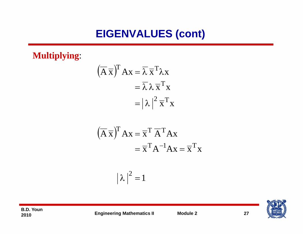
EIGENVALUES (cont)

( ) xxAxxA TT λλ=

Multiplying:

( )

xx

xx

xxAxxA

T2

T

λ

λλ=

λλ=

( ) AAAA

xx

TTT

λ=

( )xxAxAx

AxAxAxxAT1T

TT

==

=−

12 =λ


FORMS

TT

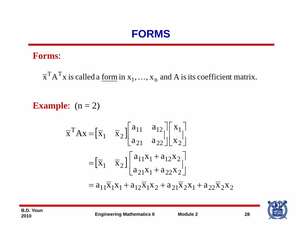
Forms:

matrix.t coefficienits isA andx,,in xforma called is xAx n1TT …

E l ( 2)Example: (n = 2)

[ ] 11211T xaaxxAxx ⎥

⎤⎢⎡

⎥⎤

⎢⎡[ ]

[ ] 212111

2222121

xaxaxx

xaaxxAxx

⎥⎤

⎢⎡ +

⎥⎦

⎢⎣

⎥⎦

⎢⎣

=

[ ]

2222122121121111

22212121

xxaxxaxxaxxa

xaxaxx

+++=

⎥⎦

⎢⎣ +

=


FORMS (cont)

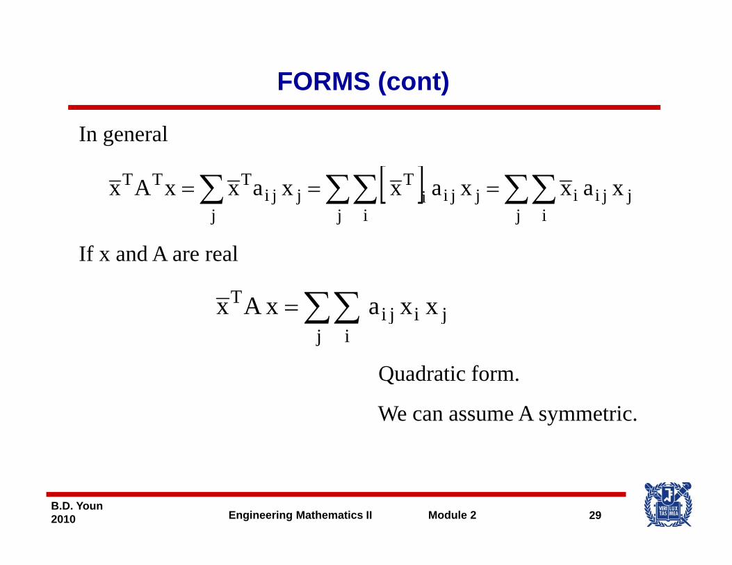
In general

[ ] ∑∑∑∑∑ TTTT

If d A l

[ ] ∑∑∑∑∑ ===j i

jjiij i

jjiiT

jjji

TTT xaxxaxxaxxAx

If x and A are real

∑∑= jijiT xxaxAx

Quadratic form.

∑∑j i

jiji

We can assume A symmetric.


QUADRATIC FORM

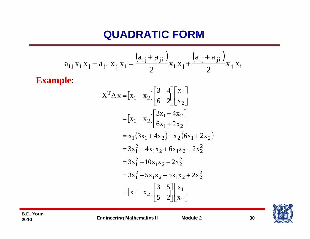
( ) ( )ij

ijjiji

ijjiijijjiji xx

2a a

xx2

a a xxa xxa

++

+=+

Example:[ ] ⎥

⎦

⎤⎢⎣

⎡⎥⎦

⎤⎢⎣

⎡=

2

121

Txx

2643

xxxAX

[ ]

( ) ( )+++

⎥⎦

⎤⎢⎣

⎡++

=

⎦⎣⎦⎣

21

2121

2

2643

x2x6x4x3

xx

( ) ( )

++=

+++=

+++=

2221

21

222121

21

212211

x2xx10x3

x2xx6xx4x3

x2x6xx4x3x

[ ] ⎥⎦

⎤⎢⎣

⎡⎥⎦

⎤⎢⎣

⎡=

+++=

121

222121

21

2211

x253

xx

x2xx5xx5x3


[ ] ⎥⎦

⎢⎣

⎥⎦

⎢⎣ 2

21 x25

QUADRATIC FORM (cont)

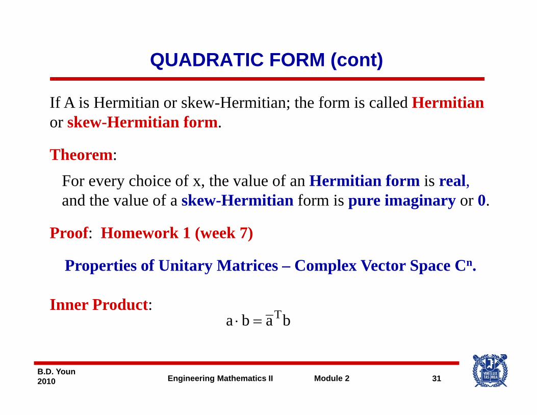
If A is Hermitian or skew-Hermitian; the form is called Hermitianor skew-Hermitian form.

Theorem: For every choice of x the value of an Hermitian form is realFor every choice of x, the value of an Hermitian form is real,and the value of a skew-Hermitian form is pure imaginary or 0.

Proof: Homework 1 (week 7)Proof: Homework 1 (week 7)

Properties of Unitary Matrices – Complex Vector Space Cn.

Inner Product: baba T=⋅



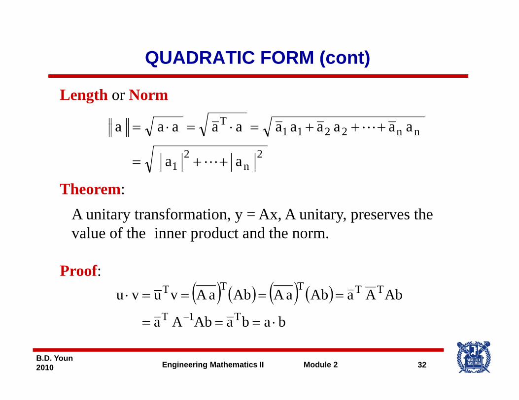
Length or NormT aaaaaaaaaaa +++

2n

21

nn2211T

aa

aaaaaaaaaaa

++=

+++=⋅=⋅=

Theorem: A unitary transformation, y = Ax, A unitary, preserves the value of the inner product and the norm.

Proof:Proof: ( ) ( ) ( ) ( )

babaAbAa

AbAaAbaAAbaAvuvuT1T

TTTTT

⋅===

====⋅−


babaAbAa


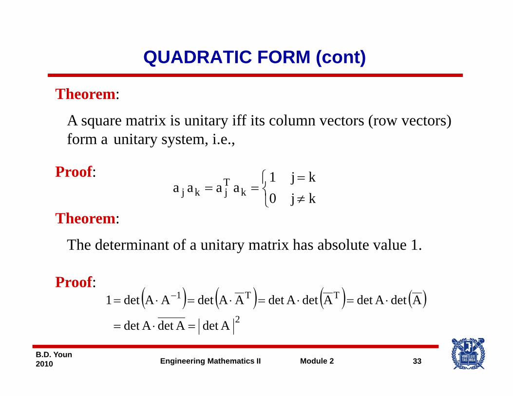
Theorem:

A square matrix is unitary iff its column vectors (row vectors)A square matrix is unitary iff its column vectors (row vectors) form a unitary system, i.e.,

Proof: ⎧ kj1Proof:

Theorem:⎩⎨⎧

≠=

==kj0kj1

aaaa kTjkj

Theorem:

The determinant of a unitary matrix has absolute value 1.

Proof:( ) ( ) ( ) ( )

2

TT1

Ad tAd tAd t

AdetAdetAdetAdetAAdetAAdet1 ⋅=⋅=⋅=⋅= −


AdetAdetAdet =⋅=

SIMULARITY OF MATRICES-BASIS OF EIGENVECTORS-DIAGONALIATION

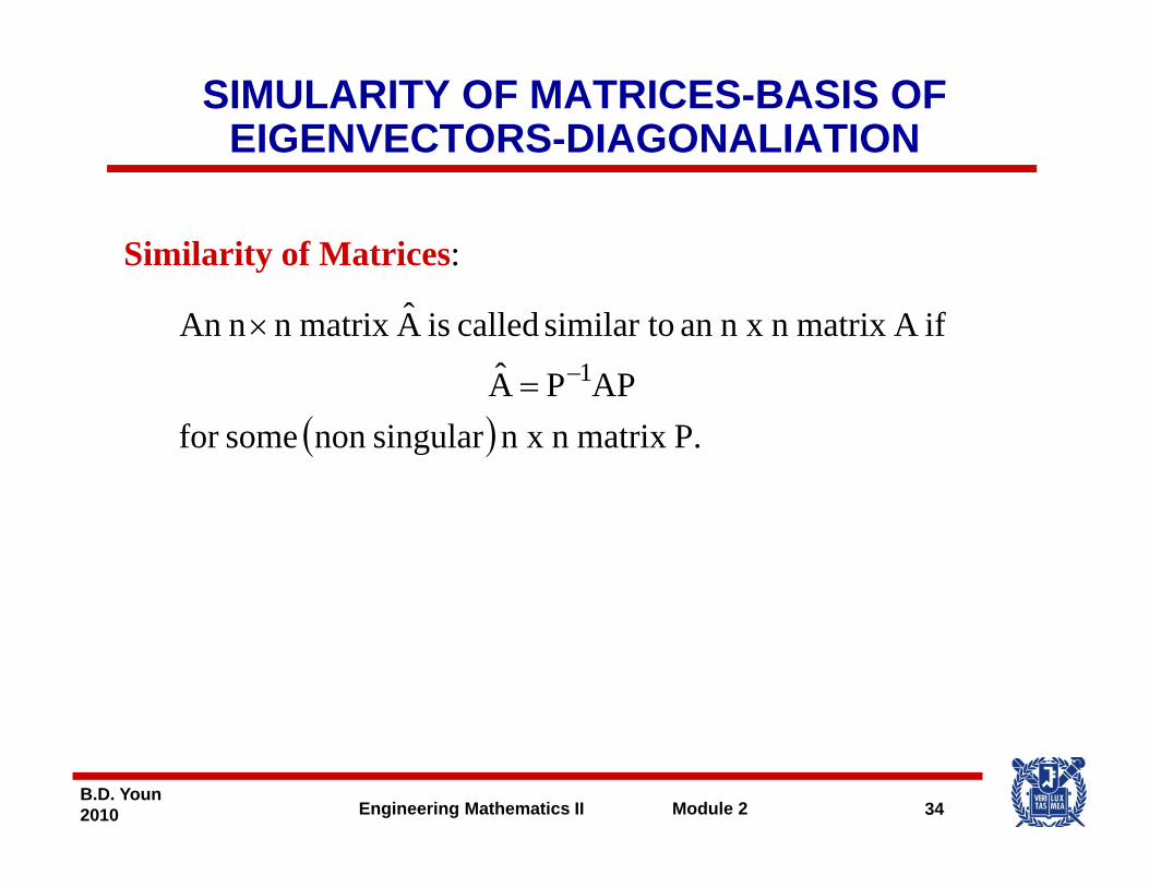
Similarity of Matrices:

APPA

ifA matrix n n x an similar to called is Amatrix n n An1−=

×

( ) P.matrix n n x singularnon somefor APPA =


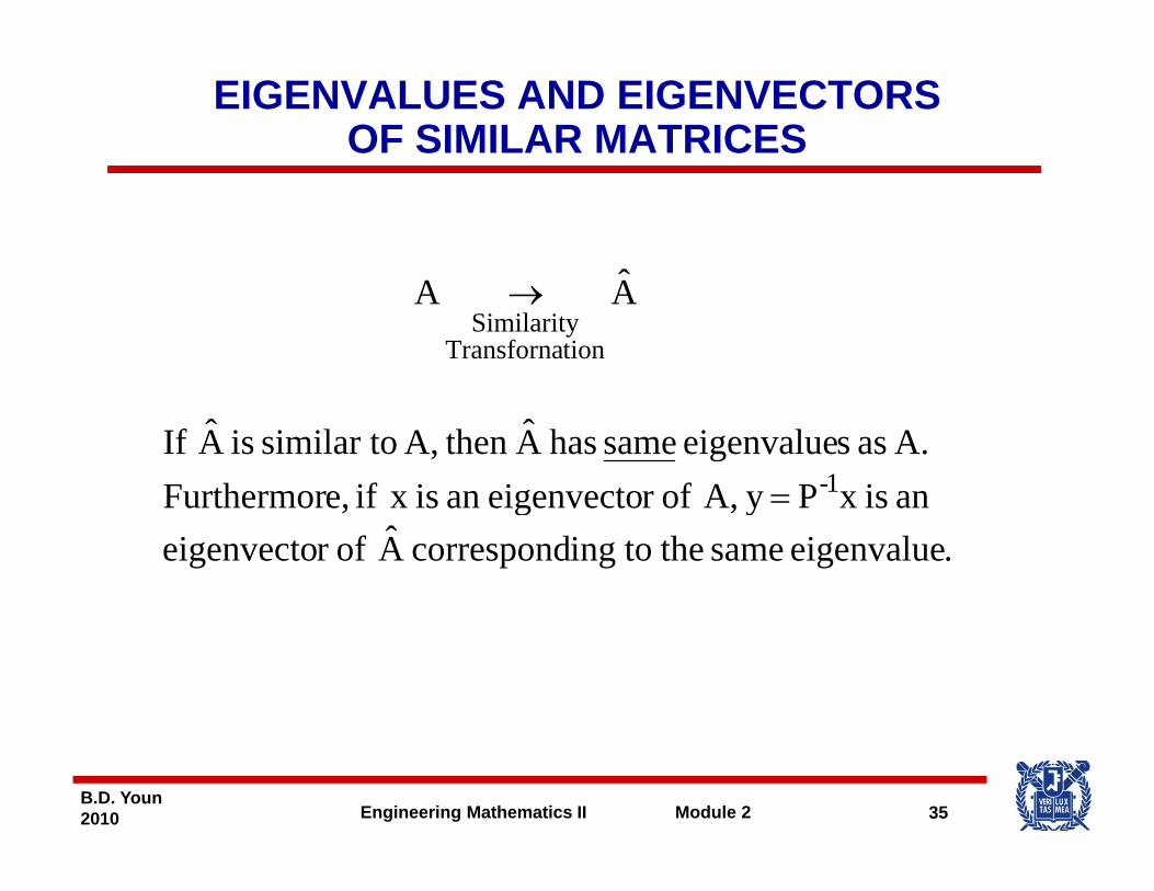
EIGENVALUES AND EIGENVECTORSOF SIMILAR MATRICES

AA tionTransforna

Similarity →

anisxPyAofreigenvectoanisxifeFurthermorA. as seigenvalue same has A then A, similar to is A If

1-=.eigenvalue same the toingcorrespond A ofr eigenvecto

an isx Py A, ofr eigenvectoan isx if e,Furthermor =


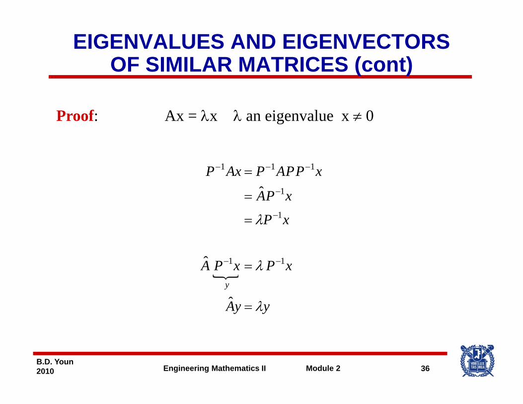
EIGENVALUES AND EIGENVECTORSOF SIMILAR MATRICES (cont)( )

Proof: Ax = λx λ an eigenvalue x ≠ 0

xPPAPAxP = −−− 111

xP

xPA

λ=

=−

−ˆ1

1

xPxPA λ= −−ˆ 11

yyAy

λ=ˆ


PROPERTIES OF EIGENVECTORS

Linear Independence

Let λ1, λ2, …, λn be distinct eigenvalues of an n × n matrix. The corresponding eigenvectors are linearly independent.

Proof

Suppose it is not the case. Let r be such that {x1, …, xr} linearly independent.

r < n


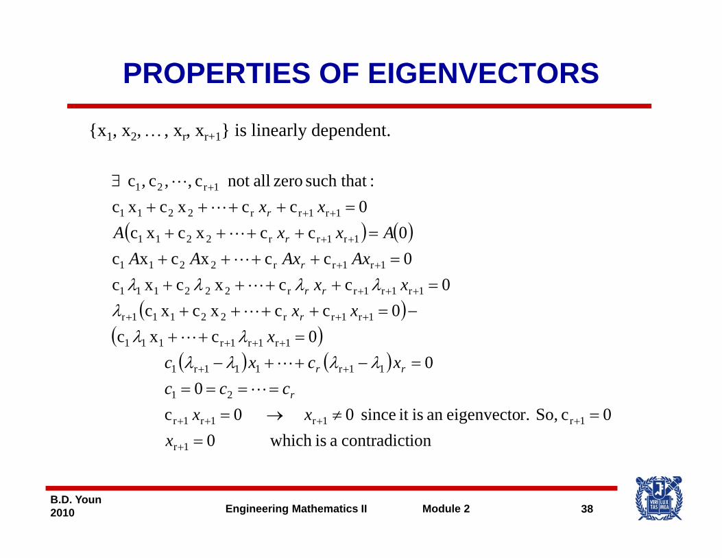
PROPERTIES OF EIGENVECTORS

{x1, x2, …, xr, xr+1} is linearly dependent.

( ) ( )0c c xc xc0c c xc xc

:such thatzeroallnot c , ,c ,c

1r1rr2211

1r1rr2211

1r21

=++++=++++

∃

++

++

+

AxxAxx

r

r

( )0ccxcxc0c c xc xc

0c c xc xc

1122111

1r1r1rr222111

1r1rr2211

−=++++=++++

=++++

+++

++

xxxx

AxAxAA

rr

r

λλλλλ

( )( )

( ) ( )0

00c xc

0ccxc xc

11r111r1

1r1r1r111

1r1rr22111r

=−++−=++++++

++

+++

+++

xcxcx

xx

rr

r

λλλλλλ

λ

ioncontradict a is which 0 0c So, r.eigenvectoan isit since 0 0c

0

1r

1r1r1r1r

21

==≠→=

====

+

++++

xxx

ccc r


BASIS OF EIGENVECTORS

If an n × n matrix A has n distinct eigenvalues then A has aIf an n × n matrix A has n distinct eigenvalues, then A has abasis of eigenvectors.

A Hermitian, skew-Hermitian or unitary matrix has a basis of, yeigenvectors that is a unitary system. A symmetric matrix hasan orthonormnal basis of eigenvectors.

(not proved here)


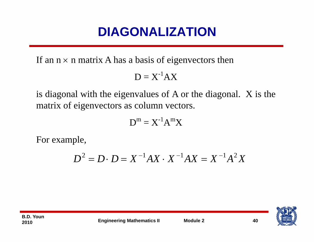
DIAGONALIZATION

If an n × n matrix A has a basis of eigenvectors then

D X-1AXD = X 1AX

is diagonal with the eigenvalues of A or the diagonal. X is thematrix of eigenvectors as column vectorsmatrix of eigenvectors as column vectors.

Dm = X-1AmX

lFor example,

XAXAXXAXXDDD 21112 −−− =⋅=⋅=


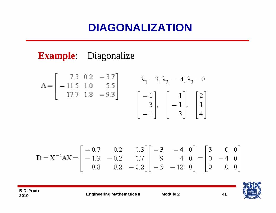
DIAGONALIZATION

Example: Diagonalize


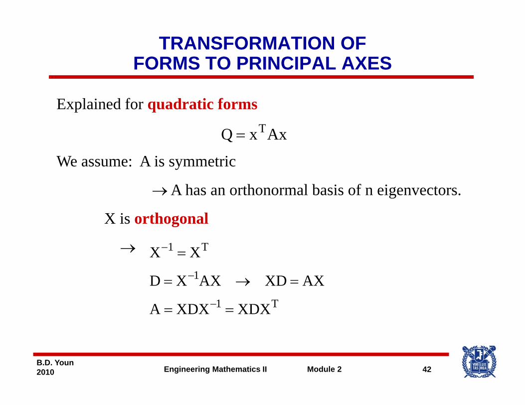
TRANSFORMATION OFFORMS TO PRINCIPAL AXES

T

Explained for quadratic forms

AxxQ T=

We assume: A is symmetric

→A has an orthonormal basis of n eigenvectors.

X is orthogonal

→

1

T1

AXXDAXXD

XX

→

=−

−

T1 XDXXDXA

AXXDAXXD

==

=→=−


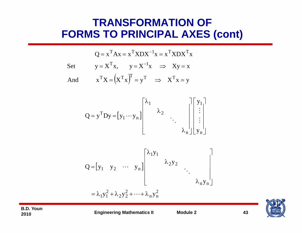
TRANSFORMATION OFFORMS TO PRINCIPAL AXES (cont)

1T

TT1TT

xXy x X y ,xXy Set

xXDXxxXDXxAxxQ

=⇒==

===−

−

( )

11

TTTTT

y

yxX yxXX x And

⎤⎡⎤⎡λ

=⇒==

[ ]1

2

1

n1T

y

y

yyDyyQ

⎥⎥⎥⎥

⎦

⎤

⎢⎢⎢⎢

⎣

⎡

⎥⎥⎥⎥

⎦

⎤

⎢⎢⎢⎢

⎣

⎡

λ

λλ

==

11

nn

y

y

⎥⎤

⎢⎡

λλ

⎦⎣⎦⎣ λ

[ ]

222

nn

22n21

y

yyyyQ

⎥⎥⎥⎥

⎦⎢⎢⎢⎢

⎣ λ

λ=


2nn

222

211 yyy λ++λ+λ=

010 141010.141 MODULE 2: Matrix Eigenvalue...

Documents

Transcript of 010 141010.141 MODULE 2: Matrix Eigenvalue...