
-regularity for systems involving non-local, antisymmetric ...armin/pdf/eps.pdf · "-regularity for...
52
ε-regularity for systems involving non-local, antisymmetric operators Armin Schikorra * May 13, 2012 We prove an epsilon-regularity theorem for critical and super-critical systems with a non-local anti- symmetric operator on the right-hand side. These systems contain as special cases, Euler-Lagrange equations of conformally invariant variational functionals as Rivi` ere treated them, and also Euler-Lagrange equations of fractional harmonic maps introduced by Da Lio-Rivi` ere. In particular, the arguments presented here give new and uniform proofs of the regularity results by Rivi` ere, Rivi` ere-Struwe, Da-Lio-Rivi` ere, and also the integrability results by Sharp-Topping and Sharp, not discriminating between the classical local, and the non-local situations. Contents 1. Introduction 1 2. L 2+ε -integrability: Proof of Theorem 1.2 6 2.1. Estimates of the H-term: Proof of Theorem 2.1 (I) ........................... 10 2.2. Better integrability for transformed potential: Proof of Theorem 2.1 (II) ............... 13 3. Higher Integrability: Proof of Theorem 1.3 17 4. Commutators and fractional product rules: Proof of Theorem 1.4 20 4.1. Pointwise fractional product rules via potentials ............................. 20 4.2. Pointwise commutator estimates via potentials ............................. 24 4.3. Fractional product rules in the Hardy-space via para-products – including the limit case ...... 30 5. Energy approach for optimal frame: Proof of Theorem 1.6 38 5.1. Preliminary propositions .......................................... 38 5.2. Energy with potentials ........................................... 40 A. Some facts on our fractional operators 46 B. Quasi-locality 48 C. Left-hand side estimates 50 D. Iteration 51 1. Introduction In recent years there has been quite some research on the effect of antisymmetric potentials in the regularity theory of critical and super-critical elliptic partial differential equations. This was initiated by Rivi` ere who in his * Max-Planck Institute for Mathematics in the Sciences, Inselstr. 22, 04103 Leipzig, Germany, [email protected]
Transcript of -regularity for systems involving non-local, antisymmetric ...armin/pdf/eps.pdf · "-regularity for...
ε-regularity for systems involving non-local,antisymmetric operators
Armin Schikorra∗
May 13, 2012
We prove an epsilon-regularity theorem for critical and super-critical systems with a non-local anti-symmetric operator on the right-hand side.These systems contain as special cases, Euler-Lagrange equations of conformally invariant variationalfunctionals as Riviere treated them, and also Euler-Lagrange equations of fractional harmonic mapsintroduced by Da Lio-Riviere.In particular, the arguments presented here give new and uniform proofs of the regularity results byRiviere, Riviere-Struwe, Da-Lio-Riviere, and also the integrability results by Sharp-Topping and Sharp,not discriminating between the classical local, and the non-local situations.
Contents
1. Introduction 1
2. L2+ε-integrability: Proof of Theorem 1.2 62.1. Estimates of the H-term: Proof of Theorem 2.1 (I) . . . . . . . . . . . . . . . . . . . . . . . . . . . 102.2. Better integrability for transformed potential: Proof of Theorem 2.1 (II) . . . . . . . . . . . . . . . 13
3. Higher Integrability: Proof of Theorem 1.3 17
4. Commutators and fractional product rules: Proof of Theorem 1.4 204.1. Pointwise fractional product rules via potentials . . . . . . . . . . . . . . . . . . . . . . . . . . . . . 204.2. Pointwise commutator estimates via potentials . . . . . . . . . . . . . . . . . . . . . . . . . . . . . 244.3. Fractional product rules in the Hardy-space via para-products – including the limit case . . . . . . 30
5. Energy approach for optimal frame: Proof of Theorem 1.6 385.1. Preliminary propositions . . . . . . . . . . . . . . . . . . . . . . . . . . . . . . . . . . . . . . . . . . 385.2. Energy with potentials . . . . . . . . . . . . . . . . . . . . . . . . . . . . . . . . . . . . . . . . . . . 40
A. Some facts on our fractional operators 46
B. Quasi-locality 48
C. Left-hand side estimates 50
D. Iteration 51
1. Introduction
In recent years there has been quite some research on the effect of antisymmetric potentials in the regularitytheory of critical and super-critical elliptic partial differential equations. This was initiated by Riviere who in his
∗Max-Planck Institute for Mathematics in the Sciences, Inselstr. 22, 04103 Leipzig, Germany, [email protected]
celebrated [Riv07] proved that solutions u ∈W 1,2(D,RN ) to the equation
∆u = Ω · ∇u in D ⊂ R2, (1.1)
which is a contracted notation of
∆ui =
N∑k=1
Ωik · ∇uk 1 ≤ i ≤ N , in D ⊂ R2,
are Holder continuous, under the condition that Ωij ∈ L2(D,R2) and the at first sight seemingly non-descriptcondition
Ωik = −Ωki, 1 ≤ i, k ≤ N. (1.2)
As Riviere showed, (1.1) with (1.2) is essentially the general form of Euler-Lagrange equations of conformallyinvariant variational functionals which allow the characterization of Gruter [Gru84], take for example a manifoldN ⊂ RN and the Dirichlet energy ˆ
R2
|∇u|2, u : D ⊂ R2 → N ⊂ RN .
We refer the interested reader to the introduction of [Riv07] for more details. In [RS08] this was generalized to anepsilon-regularity theorem for D ⊂ Rm, m ≥ 3.If the antisymmetry-condition (1.2) is violated, solutions to (1.1) might exhibit singularities such as Frehse’s [Fre73]counter-example log log 1
|x| . In fact, the antisymmetry is shown to be closely related to the appearance of Hardy
spaces, and also to Helein’s [Hel91] moving frame technique, cf. [Sch10a].Motivated by this, Da Lio and Riviere [DLR11a] (for m = 1) showed that this regularizing effect of antisymmetryexists and appears also in the setting of m/2-harmonic maps, critical points of the energy
ˆRm
∣∣∣|∇|m2 u∣∣∣2, u : Rm → N ⊂ RN .
which satisfy (roughly) an Euler-Lagrange equation of the form
∆m2 ui =
N∑k=1
Ωik |∇|m2 uk 1 ≤ i ≤ N , in D ⊂ Rm. (1.3)
Here, Ωij ∈ L2(Rm) satisfies again (1.2), and |∇|α = (−∆)α2 is the elliptic differential operator of differential order
α with the symbol |ξ|α, for the precise definition we refer to Section A .As well in the classical situation [Riv07], as also in the case of fractional harmonic maps, the argument relies ontransforming the equation with an orthogonal matrix P (in a similar way as Helein’s moving frame technique,cf. [Sch10a]). That is, one computes the respective equation P∇u instead of ∇u, or P∆
n4 u instead of ∆
n4 u and
obtains a transformed ΩP , which for the right choice of P exhibits better properties than the original Ω: In theclassical case, div(ΩP ) = 0, while in the fractional case, ΩP ∈ L2,1 (where L2,1 ( L2 is the Lorentz space dual tothe weak L2, denoted by L2,∞). Note that while a condition like div(f) = 0 is destroyed under a distortion likef := fg, even for g ∈ L∞, the condition f ∈ L2,1 is also valid for f = fg, if g ∈ L∞.Thus, the techniques developed in the fractional setting [DLR11a, DLR11b, Sch11, DL10, Sch12], seem somewhatmore dynamic and stable under certain distortions. For example, in [DLS12a, DLS12b] Da Lio and the authorwere able to extend some of the results to the degenerate situation of the energy
ˆRm||∇|αu|
mα , u : Rm → N ⊂ RN ,
the Euler-Lagrange equation of which have the form
|∇|α(||∇|αu|mα −2|∇|αu) = ||∇|αu|
mα −2
N∑k=1
Ωik |∇|αuk 1 ≤ i ≤ N , in D ⊂ Rm.
The aim of the present work is to shed more light on the connection between the two systems (1.3) and (1.1) in thecritical and supercritical case, and we are going to extend the techniques developed in [DLR11a, DLR11b, Sch11,Sch12] to give a uniform argument for ε-regularity for quite general systems which in particular include as special
2
cases both (1.3) and (1.1).
Setting w := (−∆)12u ≡ |∇|1u ∈ L2(Rn), (1.1) reads as
∆12wi =
2∑γ=1
N∑k=1
ΩγikRγ [wk], (1.4)
where Rγ ≡ ∂γ∆−12 denotes the Riesz transform. Thus, (1.1) is of the form (1.3), but Ω is not a pointwise matrix
anymore, but a non-local, linear operator mapping L2(Rm) into L1(Rm). This was our main motivation, to studythe regularity, and, in the super-critical regime, ε-regularity of solutions w ∈ L2(Rm) of
ˆwi |∇|µϕ = −
ˆΩik[wk]ϕ for all ϕ ∈ C∞0 (D), (1.5)
where Ωik is a linear mapping which maps L2(Rm) into L1(Rm). We will restrict ourselves to Ω of the form
Ωij [] =
m∑l=0
AlijRl[], (1.6)
where Alij = −Alij ∈ L2(Rm), i, j ∈ 1, . . . ,m, Rl[] is the l-th Riesz transform for l = 1, . . . ,m and R0[] is the
identity on Rm. The arguments presented here hold also for more general potentials Ω : L2 → L1, under suitableconditions on quasi-locality and its commutators. But as (1.6) contains already the most interesting examples (seebelow), we shall restrict our attention to this setting for the sake of overview.Our main result is then the following ε-regularity:
Theorem 1.1. Let µ ≤ min1, m2 or µ = m2 . Let D ⊂⊂ Rm, p ∈ (1,∞), then there exists θ > 0 such that the
following holds: Let w ∈ L2(Rm) ∩ L(2)2µ(D), that is,
‖w‖2,Rm + supBρ⊂D
ρ2µ−m
2 ‖w‖2,Bρ <∞, (1.7)
be a solution to (1.5), where Ω is of the form (1.6). If Ω satisfies moreover
supBρ(x),x∈D
ρ2µ−m
2 ‖Al‖L2 ≤ θ, (1.8)
then w ∈ Lploc(D).
Let us remark the following corollaries from Theorem 1.1.As mentioned above, by the representation (1.4) this gives a new proof of Riviere’s theorem [Riv07], and also theε-regularity theorem of [RS08].Moreover, from Theorem 1.1 a new proof of Sharp and Topping’s integrability theorem [ST11] for (1.1) follows, andalso an extension to the super-critical setting. The latter has been done independently, and by different methodsby Sharp [Sha12].
Also, we extend these integrability results to the non-local case for µ ≤ 1. For µ > 1 it seems already in theclassical setting of the biharmonic maps, cf. [Str08], that for ε-regularity we need more information on the growthof Ω in terms of the solution, a fact which appeared also in our setting and forced us to restrict µ = m
2 if µ > 1.
Another corollary worth mentioning is that the arguments presented here also enable us to treat ε-regularity criticalpoints of more general non-local energies, e.g.,
E(u) =
ˆ|∇αu|2 u : Rm → N ⊂ RN , (1.9)
where for R = [R1, . . . ,Rm]T , and Ri being the i-th Riesz transform,
∇αu := R[|∇|αu].
Another remark regards the smallness condition of (1.8). In the critical setting 2µ = m, it is easy to verify, thatthis condition holds, if D is chosen appropriately small. In the super-critical regime 2µ < m, this condition would
3
follow from some kind of monotonicity formula for stationary points of energies of the form (1.9), which for thenon-classical settings are unknown so far.
Let us now sketch the arguments we are going to need. Firstly, somewhat motivated by the arguments in [RS08],we are going estimate the growth of the norm possibly far below the natural exponent 2. More precisely weestimate the growth in R of
supBr⊂BR
rλκ−mpκ ‖w‖pκ,Br , (1.10)
starting with κ = µ, where
λκ :=m(2µ− κ)
m− κ,
pκ :=m
m− κ.
The main work is to show that for any κ ∈ [µ, 2µ) there is a good growth of these quantities, then starting forκ0 = µ, we can find a sequence of κi which converges to 2µ, such that each growth of the κi-norm (that is (1.10)with κi) is controlled by the κi−1-norm. Finally, for κ sufficiently close to 2µ, we show that we can actually havean estimate for p > 2. From this we have
Theorem 1.2. There is θ2 > 0 such that if θ < θ2, there exists p > 2, λ < 2µ, such that
w ∈ L(p)λloc (D).
For Theorem 1.2, the antisymmetry of Ω will be crucial. Once Theorem 1.2 is established, the system (1.5) becomessubcritical, and we can drop the antisymmetry condition and just by the growth of the PDE, we have
Theorem 1.3. Assume w as in Theorem 1.1, where we do not require the antisymmetry of Ω. Assume moreover,that w ∈ Lp1
loc(D) for p1 > 2. Then for any p > 2, there is θp > 0 such that if θ < θp in (1.8), also
w ∈ Lploc(D).
The main difficulty is thus Theorem 1.2 and the estimates of the Morrey norm. For the proof of this theoremwe need the following two main technical ingredients: Firstly, we need to extend the known commutator results[DLR11b, DLR11a], and also the pointwise estimates [Sch11, Sch12]. We introduce the following commutators:Let X be a linear space, For ϕ ∈ C∞0 (Rm), T : Lp(Rm) → Lq(Rm), 1 ≤ p, q ≤ ∞. We then set for f ∈ Lp(Rm)the commutator C(ϕ, T )[f ]
C(ϕ, T )[f ] := ϕT [f ]− T [ϕf ]. (1.11)
This commutator was estimated in terms of Hardy spaces for T = R the Riesz transform or T = Is the Rieszpotential in [CRW76, Cha82], nevertheless we need more precise estimates and generalizations. The next bilinearcommutator was introduced in [DLR11b], in [Sch11] pointwise estimates were given.
Hs(a, b) := |∇|s(ab)− a|∇|sb− b|∇|sa. (1.12)
For these commutators we show the following
Theorem 1.4. For any µ ∈ (0, 1], we have the following Hardy-space H estimate (for R[] any zero-multiplieroperator, we need it for the Riesz-transform, only)
‖|∇|µ(R[h] Iµb−R[h Iµb])‖H ≤ ‖h‖2 ‖b‖2
Moreover, we have‖C(f,R)[|∇|µϕ]‖2 . ‖|∇|µf‖2 [ϕ]BMO,
and its pointwise counter-part: For any δi ∈ (0, 1) and any γi ∈ (0, δi), i = 1, 2,
|C(a,R)[b]| ≤ CR,δ1,γ1 Iδ1−γ1
∣∣∣|∇|δ1a∣∣∣ Iγ1 |b|+ CR,δ2,γ2 Iγ2
(Iδ2−γ2 |b|
∣∣∣|∇|δ2a∣∣∣).Finally we have
‖Hµ(ϕ, g)‖2 . ‖|∇|µg‖2 [ϕ]BMO.
4
and‖|∇|µHµ(a, b)‖H . ‖|∇|µa‖2 ‖|∇|
µb‖2 for µ ∈ (0, 1], (1.13)
as well as its pointwise counterpart: for any µ ∈ [0,m] there is L ∈ N such that for any β ∈ [0,min(µ, 1)),µ ∈ [0,m), τ ∈ (maxβ, µ + β − 1, µ] there are, sk ∈ [0, µ), tk ∈ [0, τ), where τ − β − sk − tk ≥ 0, such that thefollowing holds ∣∣∣|∇|βHµ(a, b)
∣∣∣ . L∑k=1
Iτ−β−sk−tk(Isk ||∇|µa| Itk ||∇|
τb|).
Remark 1.5. For µ < 1 the Hardy-space estimates above follow essentially from an obvious adaption of Da Lioand Riviere’s argument [DLR11b], and (1.13) has been proven by them. For µ > 1, already from the pointwisearguments in [Sch11] there is no hope for similar results. The interesting and new case µ = 1, for which even(1.13) was unclear up to now, needs a more careful adaption of the arguments in [DLR11b].
Equipped with a good understanding of these commutator we will show
Theorem 1.6. There is a uniform Λ > 0 such that the following holds: Let Ω be as in (1.6), and assume thatΩij [] = −Ωji[]. For any Br ⊂ Rm, we can then choose P : Rm → SO(N), supp(P − I) ⊂ Br. Then for anyϕ ∈ C∞0 (Br),
−ˆ
ΩP [|∇|µϕ] ≤ C rm2 −µ ‖A‖2 [ϕ]BMO + ‖A‖22
[ϕ]BMO if µ ∈ (0, 1],
‖|∇|µϕ‖(2,∞) if µ > 1,
whereΩPij [f ] := (|∇|µPik) PTkj f + PikΩkl[P
Tlj f ],
In [Sch10a] the construction of P is done via minimization of E(P ) = ‖P∇PT + PΩP‖2L2 under the conditionthat P maps into SO(N), a.e.. This is the argument that Helein [Hel91] essentially used for his moving-frametechnique, and it provides an alternative to Riviere’s adaption of Uhlenbecks [Uhl82] gauge-theoretic constructionof P in [Riv07]. Both techniques can be extended to the fractional case, where Ω is still a pointwise multiplication[DLR11a, Sch11]. We adapt the arguments [Sch11, Sch10a] to this case of a non-local operator Ω[], by minimizingin Section 1.6 the energy
E(P ) := supψ∈L2
ˆ
Rm
ΩP [ψ],
and showing that several terms of the Euler-Lagrange equations fall under the realm of Theorem 1.4.
Notation Let Lp,q be the Lorentz spaces, cf., e.g. [Hun66, Tar07, Gra08], whose norm we denote with ‖ · ‖(p,q).We set
‖f‖(p,q)λ ≡ ‖f‖M((p,q),λ) := supBr⊂Rm
rλ−mp ‖f‖(p,q),Br , (1.14)
and for A ⊂ Rm,
[f ](p,q)λ,A := |A|λ−mmp ‖f‖(p,q),A, (1.15)
‖f‖(p,q)λ,A := supBρ⊂A
[f ](p,q),Bρ . (1.16)
We say that f belongs to the Morrey space L(p,q)λ(A), if the respective norm ‖f‖(p,q)λ,A is finite.We will also use frequently the following annuli
AkΛ,r := B2kΛr\B2k−1Λr, Akr ≡ Ak1,r. (1.17)
In Section A we recall several facts on the fractional laplacian, which we are going to use throughout this work.
Acknowledgements. The author has received funding from the European Research Council under the EuropeanUnion’s Seventh Framework Programme (FP7/2007-2013) / ERC grant agreement no 267087, DAAD PostDocProgram (D/10/50763) and the Forschungsinstitut fur Mathematik, ETH Zurich. He would like to thank TristanRiviere and the ETH for their hospitality.
5
2. L2+ε-integrability: Proof of Theorem 1.2
It is helpful, to check once and for all,
m− 2µ =m− λκpκ
, κ ∈ [µ, 2µ), (2.1)
where
λκ :=m(2µ− κ)
m− κ, (2.2)
pκ :=m
m− κ. (2.3)
Assume w : Rm → RN , µ ≤ m2 , w ∈ L2(Rm), |∇|µw ∈ L2(Rm) is for D ⊂⊂ Rm a solution to (1.5). We are going
to establish that for any κ ∈ [µ, 2µ), if θ ≡ θκ in (1.8) is suitably small, for any D ⊂⊂ D, we have
supr>0,x0∈D
rλκ−mpκ ‖w‖pκ,Br(x0) ≤ CD,w,κ. (2.4)
Note that possibly pκ < 2 for all κ ∈ [µ, 2µ). In order to show (2.4), we first note that its satisfied by assumption(1.7) for κ = µ. In fact, if x0 ∈ D ⊂⊂ D, then for any r > 0, or Br(x0) ⊂ D or r > cdist(D, ∂D). Now, weshow that for arbitrary κ ∈ [µ, 2µ), there is κ1 > κ, so that (2.4) holds. Moreover, we will show a lower bound onκ1 − κ, in order to ensure that we come arbitrarily close to 2µ if we repeat this construction finitely many times.Then we can show that if we choose κ ∈ [µ, 2µ) close enough to 2µ, (2.4) suffices to conclude the better integrabilityof Theorem 1.2.
Establishing (2.4)
For mappings P : Rm → SO(N), P ≡ I on Rm\D (denoting with I = (δij)ij ∈ RN×N the identity matrix) from(1.5) we have
ˆPikwk |∇|µϕ =
ˆwk |∇|µ(Pikϕ)−
ˆwk (|∇|µPik) ϕ−
ˆwk Hµ(Pik, ϕ)
= −ˆ
Ωkl[wl] Pikϕ−ˆwk (|∇|µPik) ϕ−
ˆwk Hµ((P − I)ik, ϕ)
Setting vi := Pikwk, this is
ˆvi |∇|µϕ = −
ˆ(PikΩkl[Pjlvj ] + (|∇|µPik)Pjkvj) ϕ−
ˆwk Hµ((P − I)ik, ϕ) (2.5)
The Growth Estimates. From (2.5), Lemma 2.2, and Lemma 2.3 we infer
Theorem 2.1 (Right-hand side estimates). If µ ∈ (0,min1, m2 ] or 2µ = m, there is a uniform Λ ≡ Λµ > 0,depending only on µ, such that the following holds: Let Br ⊂ Rm, and assume (2.5) holds for all ϕ ∈ C∞0 (Br).Then exists a choice of P such that (2.5) implies for any ϕ ∈ C∞0 (BΛ−1r), and for any τ ∈ (0, µ] sufficiently closeto, or greater than 2µ− κ,
(Λ−1r)2µ−mˆv |∇|µϕ ≤ Cκ θ ‖|∇|τϕ‖( m
τ+κ−µ ,1)‖w‖(pκ,∞)λκ ,Br
+Cκ θ ‖|∇|τϕ‖( mτ+κ−µ ,2)
Λκ−3µ∞∑k=1
2k(κ−3µ) [w](pκ,∞)λκ ,Akr.
where we recall that the right-hand side norms were defined in (1.15), (1.16), Akr is as in (1.17), and λκ as in(2.2), pκ as in (2.3).
6
From Theorem 2.1 and Lemma C.1 (applied to Λ−1r instead of r) we infer for any τ ∈ (0, µ] sufficiently closeto µ and any Λ Λµ sufficiently large (for the right-hand side norms recall (1.15) and (1.16)), also in view ofProposition A.7,
(Λ−2r)2µ−m ‖|∇|µ−τv‖( mm+µ−τ−κ ,∞),BΛ−2r
≤ Λ−1 Cκ θ ‖w‖(pκ,∞)λκ ,Br
+Λ−1 Cκ θ
∞∑k=1
2k(κ−3µ) [w](pκ,∞)λκ ,Akr.
+C (Λ−2r)2µ−m Λκ−m+τ−µ‖w‖(pκ,∞),BΛ−1r
+C (Λ−2r)2µ−m Λκ−m+τ−µ∞∑k=0
2k(κ−m+τ−µ) ‖w‖(pκ,∞),AkΛ−1r
(2.1)
≤ Cκ θ Λm−2µ ‖w‖(pκ,∞)λκ ,Br
+Cκ θ Λm−2µ∞∑k=1
2k(κ−3µ) [w](pκ,∞)λκ ,Akr
+C Λκ+τ−3µ ‖w‖(pκ,∞)λκ ,BΛ−1r
+C Λκ+τ−3µ∞∑k=0
2k(κ+τ−3µ) [w](pκ,∞)λκ ,AkΛ−1r
P.A.7
. (Cκ θ Λm−2µ + CΛκ+τ−3µ) ‖w‖(pκ,∞)λκ ,Br
+(Cκ θ Λm−2µ + C Λκ+τ−3µ)
∞∑k=1
2k(κ+τ−3µ) [w](pκ,∞)λκ ,Akr.
For later reference, we write this as
(Λ−2r)2µ−m ‖|∇|µ−τv‖( mm+µ−τ−κ ,∞),BΛ−2r
≤ (Cκ,µ θ Λm−2µ + Cµ Λκ+τ−3µ) ‖w‖(pκ,∞)λκ ,Br
+(Cκ,µ θ Λm−2µ + Cµ Λκ+τ−3µ)
∞∑k=1
2k(κ+τ−3µ) [w](pκ,∞)λκ ,Akr.
(2.6)For τ = µ,
(Λ−2r)2µ−m ‖v‖(pκ,∞),BΛ−2r≤ (Cκ,µ θ Λm−2µ + Cµ Λκ−2µ) ‖w‖(pκ,∞)λκ ,Br
+(Cκ,µ θ Λm−2µ + Cµ Λκ−2µ)
∞∑k=1
2k(κ−2µ) [w](pκ,∞)λκ ,Akr.
(2.7)
The Iteration Procedure. Note that |w| = |v|, so we can use them equivalently. Equation (2.7) holds for anyBr(x0), where x0 ∈ D and r < d(x0) := C dist(x0, ∂D) (the constant essentially only depending on the constructionof P and the set where Ω is small). For x0 ∈ D and R > 0 set
Φx0(R) := sup
Bρ⊂BR(x0)
ρ2µ−m‖w‖(pκ,∞),Bρ,
and its centered counter-part
Ψx0(R) := sup
ρ∈(0,R)
ρ2µ−m‖w‖(pκ,∞),Bρ(x0) ≤ Φx0(R)
then from (2.7) for any R, x0 ∈ D with R < d(x0), we have
Φx0(Λ−1R) ≤(Cκ θΛ
m−2µ + C Λκ−2µ)
Φx0(R) +(Cκ θΛ
m−2µ + C Λκ−2µ) ∞∑k=1
2k(κ−2µ) Ψx0(2kR).
7
Note that from (2.4), we know that Φx0(R) < CD,x0,w for any x0 ∈ D. Now we can iterate, Lemma D.1, satisfying
the assumption (D.1) by choosing Λ ≡ Λκ := 2Cµ
(2µ−κ)4 with sufficiently large Cµ and assuming that θ < (Λκ)κ−m.Then, for any r < R,
supBρ⊂Br(x0)
ρ2µ−m ‖w‖(pκ,∞),Bρ= supBρ⊂Br(x0)
ρ2µ−m ‖v‖(pκ,∞),Bρ. Cκ,w,Λ,R rσκ , where σκ = (2µ−κ)4
Cµ.
We can assume, that σκ < 2µ− κ. Since
supρ>R
r2µ−σκ−m ‖w‖(pκ,∞),Br(x0) . R−σκ ‖w‖(pκ,∞)λκ ,B4r,
we arrive atr2µ−σκ−m ‖w‖(pκ,∞),Br(x0) ≤ Cκ,w,x0
so we get for any Br(x0) ⊂ BR(x0)
r−σκ‖χBrw‖(pκ,∞)λκ+ supρ>0
ρ2µ−σκ−m‖w‖(pκ,∞),Bρ(x0) ≤ Cκ,w.
Plugging this into (2.6), we have for all τ ∈ (0, µ] sufficiently close to, or greater than 2µ− κ,
r2µ−m ‖|∇|µ−τv‖( mm+µ−τ−κ ,∞),BΛ−1r(x0) . Cκ,wr
σκ + Cκ,w rσκ∞∑k=1
2k(κ−2µ+σκ), (2.8)
so that we have for all small r,
r2µ−m−σκ ‖|∇|µ−τv‖( mm+µ−τ−κ ,∞),Br(x0) . Cw,κ,R.
Moving the BR(x0), for any D1 ⊂⊂ D, we have that
‖|∇|µ−τv‖( mm+µ−τ−κ ,∞)λ,D1
. Cw,κ,|∇|1,D (2.9)
for λ such that (choosing τ possibly even closer to µ, ensuring that |µ− τ | ≤ σκ2 )
λ
m=
3µ− τ − κ− σκm+ µ− τ − κ
≤ 3µ− τ − κ− σκm− κ
(2.2)=
λκm
+µ− τ − σκm− κ
Choosing the next κ. Assume for a moment that 2µ < m. we can guarantee
0 < λ < λκ − cmσκ, (2.10)
and we choose κ1,1 ∈ (κ, 2µ) via
λ =: m2µ− κ1,1
m− κ1,1.
By (2.10),
m2µ− κ1,1
m− κ1,1< m
2µ− κm− κ
− cm−2µ σκ
and thus we have
κ1,1 > κ+ σcm−2µ(m− κ1,1)(m− κ)
m.
On the other hand, by a localized version of Adams’ [Ada75]-argument on Riesz potentials, we infer from (2.9)that for any D2 ⊂⊂ D1,
‖v‖(p,∞)λ,D2= ‖w‖(p,∞)λ,D2
<∞,
where1
p=m+ µ− τ − κ
m− µ− τ
λ∈ (0, 1).
Lettingm
m− κ1,2:= p,
8
we can estimateκ1,2 − κm
= (µ− τ)
(1
λ− 1
m
)≥ σκcµ.
Thus for a certain α > 0,κ1 := minκ1,1, κ1,2 ≥ κ0 + c0(2µ− κ)α,
and since
p ≥ m
m− κ1, λ < m
2µ− κ1
m− κ1,
for any D3 ⊂⊂ D, we arrive at‖w‖(pκ1
,∞)m
2µ−κ1m−κ1
,D3<∞.
Varying this in D3 ⊂⊂ D, we have (2.4) for κ1. If 2µ = m, we use this same argument, to conclude that w ∈ Lp(D3)for some p > 2, which is already the claim of Theorem 1.2.
Estimating the growth of κ. Iterating this procedure (for smaller and smaller θ in (1.8)), we obtain κk ∈ [µ, 2µ),and
κk+1 ≥ κk + c0(2µ− κ)α.
Since the sequence (κk)k is monotone and bounded, and the only fixed point is κ∞ = 2µ, for any ε > 0 there is astep-count L such that |κL − 2µ| < ε. This shows (2.4).
Integrability slightly above 2
By the arguments above, fixing D ⊂⊂ D, going back to (2.8), if 2µ− κ < ε small enough, for τ ∈ (ε, µ], ignoringσκ > 0,
supBr⊂D
r2µ−m ‖|∇|µ−τv‖( mm+µ−τ−κ ,∞),BΛ−1r(x0) . Cκ,w,D.
If 2µ = m, choosing τ = µ, we havem
m+ µ− µ− κκ→2µ=m−−−−−−→∞,
which proves Theorem 1.2, and in fact even Theorem 1.1. So let from now on 2µ < m, µ ≤ 1. Then for λs,ε ∈ (0,m),s := µ− τ ,
λs,ε −mm
m+µ−τ−κ= 2µ−m
⇔ λs,ε =m
m+ µ− τ − κ(3µ− τ − κ)
τ→µ,κ→2µ−−−−−−−→ 0
and1
p:=
m+ µ− τ − κm
− µ− τm
m+µ−τ−κ (3µ− τ − κ)=m+ µ− τ − κ
m− (µ− τ)(m+ µ− τ − κ)
m(3µ− τ − κ)
= 1 +µ− τ − κ
m(3µ− τ − κ)(2µ+ τ − κ)− (µ− τ)
3µ− τ − κwe have by Adams’ [Ada75],
v ∈ L(p,∞)λs,εloc (D).
One checks that there is ε > 0 such that if |τ − µ| < ε, 2κ− µ < ε, then p > 2, λs,ε < 2µ.
9
2.1. Estimates of the H-term: Proof of Theorem 2.1 (I)
This is to estimate for ϕ ∈ C∞0 (Br) the following term
ˆw Hµ(P − I, ϕ) =
ˆIβw |∇|βHµ(P,ϕ) (2.11)
Lemma 2.2. Let µ ∈ (0, m2 ], µ ≤ 1 or µ = m2 . For any κ ∈ [µ, 2µ), there are Cκ,µ > 0, τ ∈ (0, µ) such for any
ϕ ∈ C∞0 (BΛ−1r) the following holds: If supp(P − I) ⊂ BΛ−1r,
(Λ−1r)2µ−mˆw Hµ(P − I, ϕ) ≤ Cκ,µ ‖|∇|τϕ‖( m
κ+τ−µ ,2) (Λ−1r)µ−m2 ‖|∇|µP‖2 ‖w‖(pκ,∞)λκ ,Br
+Cκ,µ ‖|∇|τϕ‖( mκ+τ−µ ,2) (Λ−1r)µ−
m2 ‖|∇|µP‖2
∞∑k=1
(2kΛ)κ−3µ[w](pκ,∞)λκ ,Akr
where we recall the definition Akr from (1.17), λκ from (2.2), and pκ from (2.3). As for the asymptotic behavioras κ→ 2µ, one can choose τ approaching maxµ− 1, 0, and Cκ,µ blows up.
Proof of Lemma 2.2. For a somewhat clearer presentation, we are going to show the following claim for ϕ ∈C∞0 (Br) and supp(P − I) ⊂ Br
r2µ−mˆw Hµ(P − I, ϕ) ≤ Cκ,µ ‖|∇|τϕ‖( m
κ+τ−µ ,2) rµ−m2 ‖|∇|µP‖2 ‖w‖(pκ,∞)λκ ,BΛr
+Cκ,µ ‖|∇|τϕ‖( mκ+τ−µ ,2) r
µ−m2 ‖|∇|µP‖2∞∑k=1
(2kΛ)κ−3µ[w](pκ,∞)λκ ,AkΛ,r.
Applied to r := Λ−1r gives the original claim.
As usual, we decompose ˆw Hµ(P − I, ϕ) = I +
∞∑k=1
IIk,
where
I :=
ˆχBΛr
w Hµ(P − I, ϕ),
and, denoting Ak := AkΛ,r,
IIk :=
ˆw Hµ(P − I, ϕ)χAk .
As for IIk, since suppϕ ∪ supp(P − I) ⊂ Br
Hµ(P − I, ϕ)χAk = χAk |∇|µ((P − I)ϕ).
By Lemma B.1 we then have for any τ ∈ (0, µ], using also Lemma A.5,
‖Hµ(P − I, ϕ)‖(mκ ,1).Ak.
(2kΛr
)−m−µ (2kΛr
)κrm2 −κ+µ ‖ϕ‖( m
κ−µ ,∞) ‖P − I‖2
.(2kΛr
)−m−µ (2kΛr
)κrm2 −κ+2µ‖|∇|τϕ‖( m
κ+τ−µ ,∞) ‖|∇|µP‖2
=(2kΛ
)−m+κ−µ ‖|∇|τϕ‖( mκ+τ−µ ,∞) r
µ−m2 ‖|∇|µP‖2.
Consequently,
|IIk| . ‖wχAk‖(pκ,∞)
(2kΛ
)−m+κ−µ ‖|∇|τϕ‖( mκ+τ−µ ,∞) r
µ−m2 ‖|∇|µP‖2(2.1)
. (2kΛr)m−2µ [wχAk ](pκ,∞)λκ
(2kΛ
)−m+κ−µ ‖|∇|τϕ‖( mκ+τ−µ ,∞) r
µ−m2 ‖|∇|µP‖2
. rm−2µ (2kΛ)κ−3µ ‖|∇|τϕ‖( mκ+τ−µ ,∞) r
µ−m2 ‖|∇|µP‖2 [wχAk ](pκ,∞)λκ.
10
As for I, set w := χBΛrw and write ˆw Hµ(P,ϕ) =
ˆIβw |∇|βHµ(P,ϕ)
Actually, the claim follows quite straight forward from (4.18) for µ ≤ 1, β := µ, but the pointwise estimates on H,Lemma 4.1, are strong enough to deal with our situation, and they do not make use of para-products which werenecessary for the proof of (4.18): By Lemma A.6
‖Iβw‖(p1,∞)λκ. ‖w‖(pκ,∞)λκ
where for β < min(2µ− κ, 1),1
p1=m− κm
2µ− κ− β2µ− κ
∈ (0, 1).
If µ = m2 , we set β = 0, if µ < m
2 , let ε > 0 such that µ + ε < m2 . Now we estimate ||∇|βHµ(P,ϕ)|, applying
Lemma 4.1 for any τ ∈ (maxβ, µ + β − 1, µ], we have to control terms of the form (for s ∈ (0, µ), t ∈ (0, τ),τ − β − s− t ∈ [0, ε))
Iτ−β−s−t(Is||∇|µP | It||∇|τϕ|).We have
‖Is||∇|µP |‖(p2,2) . ‖|∇|µP‖2,
1
p2=
1
2− s
m∈ (0, 1),
‖It||∇|τϕ|‖(p3,2) . ‖|∇|τϕ‖( m
κ+τ−µ ,2),1
p3=κ+ τ − µ
m− t
m∈ (0, 1).
Note that
0 <1
p2+
1
p3=
1
2+κ+ τ − µ− s− t
m<
1
2+κ+ τ − µ+ ε− τ + β
m<
1
2+ε+ µ
m< 1,
consequently,‖Iτ−β−s−t(Is||∇|µP | It||∇|τϕ|)‖(p4,1) . ‖|∇|
µP‖2 ‖|∇|
τϕ‖( m
κ+τ−µ ,2),
where1
p4=
1
p2+
1
p3− τ − β − s− t
m=
1
2+κ+ β − µ
m∈ (0, 1).
Now we have to ensure that the f(β) ≤ 1 for admissible β (and admissible τ):
f(β) :=1
p1+
1
p4=
3
2− µ
m− β m− 2µ
m(2µ− κ)> 0.
Obviously, f(0) = 1 holds, if µ = m2 (so β = 0, and τ arbitrarily between (µ−1, µ]). As for the case µ < m
2 , µ ≤ 1,We have 2µ− κ ≤ 1 for κ ∈ [µ, 2µ), then
f(2µ− κ) =1
2+µ
m< 1.
so we can take β < 1 sufficiently close to 2µ − κ, so that f(β) < 1, and take τ ∈ (β, µ) sufficiently close to orgreater than 2µ− κ. Consequently,
|I| .ˆB4r
Iβw |∇|βHµ(P,ϕ) +
∞∑k=1
ˆAk4r
Iβw |∇|βHµ(P,ϕ)
. ‖Iβw‖(p1,∞),B4r‖|∇|βHµ(P,ϕ)‖(p4,1) r
m− mp1− mp4
+
∞∑k=1
‖Iβw‖(p1,∞),Ak4r‖|∇|βHµ(P,ϕ)‖(p4,1),Ak4r
(2kr)m−mp1− mp4
. rm−λκp1 ‖Iβw‖(p1,∞)λκ
‖|∇|βHµ(P,ϕ)‖(p4,1) rm− m
p1− mp4
+
∞∑k=1
(2kr)m−λκp1 ‖Iβw‖(p1,∞)λκ
‖|∇|βHµ(P,ϕ)‖(p4,1),Ak4r(2kr)m−
mp1− mp4
. rm−λκp1 ‖w‖(pκ,∞)λκ
‖|∇|βHµ(P,ϕ)‖(p4,1) rm− m
p1− mp4
+
∞∑k=1
(2kr)m−λκp1 ‖w‖(pκ,∞)λκ ,A
k4r‖|∇|βHµ(P,ϕ)‖(p4,1),Ak4r
(2kr)m−mp1− mp4 .
11
By Proposition 4.3, for the same τ as above,
‖|∇|βHµ(P,ϕ)‖(p4,1) . ‖|∇|µP‖2 ‖|∇|
τϕ‖ m
κ−τ−µ ,2.
Now we apply Proposition 4.4 (using that ϕ and P − I have support in Br), and using
m− m(2µ−κ)m−κp1
+m− m
p1− m
p4−m− β +
m
p4
= −2µ+ κ,
andm− λκp1
+m− m
p1− m
p4+m
2− µ = m− 2µ
we conclude
|I| . rm−2µ ‖w‖(pκ,∞)λκrµ−
m2 ‖|∇|µP‖2 ‖|∇|
τϕ‖ m
κ−τ−µ ,2
+rm−2µ∞∑k=1
2k(−2µ+κ)‖w‖(pκ,∞)λκ ,Ak4r‖|∇|τϕ‖( m
κ+τ−µ ,∞) rµ−m2 ‖|∇|µP‖(2,∞)
. Cκrm−2µ ‖wχBΛr
‖(pκ,∞)λκrµ−
m2 ‖|∇|µP‖2 ‖|∇|
τϕ‖ m
κ−τ−µ ,2.
12
2.2. Better integrability for transformed potential: Proof of Theorem 2.1 (II)
This section is devoted to the proof of the following Lemma:
Lemma 2.3. Let Br ⊂ Rm, Ω as in (1.6), Λ > 2. There exists P : Rm → SO(N), P ≡ I on Rm\BΛ−1r, with theestimate
(Λ−1r)2µ−m
2 ‖|∇|µP‖2,Rm . θ, (2.12)
such that for any τ ∈ (0, µ] sufficiently close or greater than 2µ− κ, κ ∈ [µ, 2µ), θ > 0 from (1.8) in D = Br, andfor any ϕ ∈ C∞0 (BΛ−1r), if µ ∈ (0, 1], or µ = m
2 ,
(Λ−1r)2µ−mˆ (
(|∇|µP )PTw + PΩ[PTw])ϕ ≤ Cκ,µ θ ‖|∇|τϕ‖( m
κ+τ−µ ,1) ‖w‖(pκ,∞)λκ ,Br
+Cκ,µ θ ‖|∇|τϕ‖( mκ+τ−µ ,2)
∞∑k=1
(2kΛ)κ−3µ [w](pκ,∞)λκ ,Akr.
where we recall the definition Akr from (1.17), λκ from (2.2), and pκ from (2.3).
As in the proof of Lemma 2.2, we prove the scaled claim for replacing r by Λr which makes the presentation ofthe proof somewhat lighter: We are going to show the existence of P such that for ϕ ∈ C∞0 (Br)
r2µ−mˆ (
(|∇|µP )PTw + PΩ[PTw])ϕ ≤ Cκ,µ θ ‖|∇|τϕ‖( m
κ+τ−µ ,1) ‖w‖(pκ,∞)λκ ,BΛr
+Cκ,µ θ ‖|∇|τϕ‖( mκ+τ−µ ,2)
∞∑k=1
(2kΛ)κ−3µ [w](pκ,∞)λκ ,AkΛ,r,
(2.13)
Fix Br ⊂ Rm. In order to prove this claim, note thatˆ (
(|∇|µP )PTw + PΩ[PTw])ϕ =
ˆ ((|∇|µP )PTw + PχBrΩ[PTw]
)ϕ,
so we are going to assume that the Al in (1.6)
suppAl ⊂ Br, Ω[] = χBrΩ[] (2.14)
and consequently assuming (from (1.8)) that
r2µ−m
2 ‖Al‖2,Rm ‖f‖2 + supρ∈(0,Λr)
ρ2µ−m
2 ‖Ω[f ]‖1,Bρ . θ ‖f‖2 (2.15)
Let P : Rm → SO(N) be the minimizer, P ≡ I on Rm\Br, of E(·) ≡ Er,x,Λµ,1,2(·), where Λµ is from Lemma 5.5.Using (5.7), (2.14), we have the estimates (for from now on fixed Λ > 2),
r2µ−m
2 ‖|∇|µP‖2,Rm . θ, (2.16)
which after rescaling amounts to (2.12), and with the help of (2.15),
r2µ−m
2
∥∥(|∇|µP )PT f + PΩ[PT f ]∥∥
1,BΛr. θ ‖f‖2,Rm . (2.17)
Let
w = wχBΛr+
∞∑k=1
wχAkΛr =: w0 +
∞∑k=1
wk.
Then, ˆ ((|∇|µP )PTw + PΩ[PTw]
)ϕ
=
ˆ(|∇|µP )PTw0ϕ+ PΩ[PTw0ϕ] −
ˆPC(ϕ,Ω)[PTw0] +
∞∑k=1
ˆPΩ[PTwk] ϕ
=: I − II + III.
13
The disjoint support part (III)
Since µ ≤ κ < 2µ,
ˆPΩ[PTwk] ϕ
(1.6)
. ‖A‖2,Br ‖ϕ‖2 ‖R[PTwk]‖∞,BrP.B.1
. ‖A‖2,Br rm2 −κ+µ ‖|∇|τϕ‖ m
κ+τ−µ(2kΛr)−m+κ ‖wk‖(pκ,∞)
(2.1)
. rµ−m2 ‖A‖2,Br ‖|∇|
τϕ‖ m
κ+τ−µ(2kΛ)−m+κ (2kΛr)m−2µ [w](pκ,∞)λκ ,A
kΛ,r
(2.15)
. θ rm−2µ (2kΛ)κ−2µ ‖|∇|τϕ‖ mκ+τ−µ
[w](pκ,∞)λκ ,AkΛ,r.
The same-support/commutator part (II)
We have
|II| . ‖A‖2 ‖C(ϕ,R)[PTw0]‖2,Br(2.15)
. rm−2µ
2 θ ‖C(ϕ,R)[PTw0]‖2,Br .
Now we apply Lemma 4.7, and have for arbitrary δ ∈ (0, 1), γ1,2 ∈ (0, δ),∣∣C(ϕ,R)[PTw0]∣∣ . Iδ−γ1
||∇|δϕ| Iγ1|w0|+ CR,δ,γ2
Iγ2
(||∇|δϕ| Iδ−γ2
|w0|)
Now, if we choose δ < τ‖Iδ1−γ1
||∇|δ1ϕ|‖( mγ1+κ−µ ,q)
. ‖|∇|τϕ‖( mτ+κ−µ ,q)
,
and for β < 2µ− κ, using [Ada75], see Lemma A.6,
rλκ−mpγ1 ‖Iβw0‖(pβ ,∞),Br
. ‖Iβw0‖(pβ ,∞)λκ. ‖w0‖(pκ,∞)λκ
where1
pβ=m− κm
2µ− κ− β2µ− κ
∈ (0, 1).
Now,
1
pγ1
+γ1 + κ− µ
m
=µ
m+ (m− 2µ)
(2µ− κ)− γ1
m(2µ− κ)
≤ 1
2,
(2.18)
if we choose γ1 ∈ (0, 2µ− κ) as follows: If µ = m2 we can choose γ arbitrarily. If µ < m
2 and µ ≤ 1, then we pickγ1 sufficiently close to 2µ− κ ≤ 1. That is, for any τ < µ sufficiently close or greater than 2µ− κ such that thereis a γ1 < δ < τ , δ < 2µ− κ, satisfying the above equation, we have
‖Iδ−γ1 ||∇|δ1ϕ| Iγ1 |w0|‖2,Br . r
m2 −
mpγ1−(γ1+κ−µ)
rm−λκpγ1 ‖|∇|τϕ‖( m
τ+κ−µ ,2) ‖w0‖(pκ,∞)λκ,
andm
2− m
pγ1
− (γ1 + κ− µ) +m− λκpγ1
=m
2− (γ1 + κ− µ)− (2µ− κ− γ1) =
m
2− µ.
As for the second term, for δ − γ2 < 2µ− κ, using the formula (2.18) with δ instead of γ1,
1
p2:=
δ + κ− µm
+1
pδ−γ2
=δ + κ− µ
m+
1
pδ+ γ2
m− κm(2µ− κ)
≤ 1
2+ γ2
m− κm(2µ− κ)
< 1,
if we choose γ1 < δ (as above γ1) close enough 2µ− κ, and γ2 very small. Consequently, if we set
λ := λκ,
14
and λ ∈ (0,m) such that λ−mp2
= λ−mpδ−γ2
, that is
λ
p2=λ−mpδ−γ2
+m
p2=λκ −mpδ−γ2
+ δ + κ− µ+m
pδ−γ
= (λκ)m− κm
2µ− κ− (δ − γ2)
2µ− κ+ δ + κ− µ
= µ+ γ2
(2.19)
then
‖|∇|δ2ϕ Iδ2−γ2|w0|‖(p2,2)λ
≈ supBρ
ρλ−mp2 ‖||∇|δ2ϕ| Iδ2−γ2
|w0|‖(p2,2),Bρ
. ‖|∇|τϕ‖( mτ+κ−µ ,2) sup
Bρ
ρλ−mp2 ‖Iδ2−γ2
|w0|‖(pδ2−γ2,∞),Bρ
≈ ‖|∇|τϕ‖( mτ+κ−µ ,2) ‖Iδ2−γ2 |w0|‖(pδ2−γ2
,∞)λ,Bρ
. ‖|∇|τϕ‖( mτ+κ−µ ,2) ‖w0‖(pκ,∞)λκ
.
Now observe1
2−(
1
p2− γ2
λ
)(2.19)
=1
2− µ
p2(µ+ γ2)
=1
2− µ
µ+ γ2
(δ2 + κ− µ
m+m− κm
2µ− κ− (δ2 − γ2)
2µ− κ
)=
1
2− µ
µ+ γ2
(((2µ− κ)− δ2)
m− 2µ
m(2µ− κ)+µ
m+m− κm
γ2
2µ− κ
)≥ 0,
for sufficiently small γ2 and δ2 sufficiently close to 2µ − κ. In fact, this holds obviously, if µm < 1
2 . If µm = 1
2 , wehave
µ
µ+ γ2
(((2µ− κ)− δ2)
m− 2µ
m(2µ− κ)+µ
m+m− κm
γ2
2µ− κ
)=
µ
µ+ γ2
(1
2+γ2
2µ
)=
1
2
Moreover, one checks
m
2− µ
µ+ γ2
m
p2+
µ
µ+ γ2
m− λp2
=m
2− µ
µ+ γ2
λ
p2
(2.19)=
m
2− µ.
Thus,
‖Iγ2(|∇|δ2ϕ Iδ2−γ2
|w0|)‖2,Br . rm2 −µ ‖Iγ2
(|∇|δ2ϕ Iδ2−γ2|w0|)‖( p2(µ+γ2)
µ ,2)λ
. rm2 −µ ‖|∇|δ2ϕ Iδ2−γ2 |w0|‖(p2,2)λ
. rm2 −µ ‖|∇|τϕ‖( m
τ+κ−µ ,2) ‖w0‖(pκ,∞)λκ.
The same-support/commutator part (I)
Here, we decompose
w0ϕ = |∇|µ(ηΛr(Iµ(w0ϕ))) + |∇|µ((1− ηΛr)(Iµ(w0ϕ))) =: |∇|µg1 + |∇|µg2
and
I =
ˆ(|∇|µP )PT |∇|µg1 + PΩ[PT |∇|µg1] +
ˆ(|∇|µP )PT |∇|µg2 + PΩ[PT |∇|µg2]
=: I1 + I2.
15
For I1 we use Theorem 1.6 in the form of Lemma 5.7,
I1 =
ˆΩP [|∇|µg1] . θ rm−2µ
[g1]BMO if µ ≤ 1,
rµ−m2 ‖|∇|µg1‖(2,∞) if µ > 1.
Note thatsupp(ϕw0) ⊂ Br,
and moreover for qµ =∞, for κ > µ, and qµ = 1 for κ = µ, (for arbitrary τ > 0)
‖ϕw0‖( mm−µ ,∞) µm
m−µ. ‖ϕ‖( m
κ−µ ,∞)‖wχBr‖(pκ,∞)λκ. ‖|∇|τϕ‖( m
κ+τ−µ ,qµ)‖w‖(pκ,∞)λκ ,B2r. (2.20)
Then, the claim for I1 follows from
Proposition 2.4. Let µ ≤ 1, g := ηΛrIµ(f), supp f ⊂ Br, then for any κ ∈ [µ, 2µ),
[g]BMO .(1 + Λµ−m
)‖f‖( m
m−µ ,∞) µmm−µ
.
Proof. From [Ada75, Proposition 3.3.][g]BMO . ‖|∇|µg‖(1)µ
.
Since,|∇|µg = f + |∇|µ((1− ηΛr)Iµf),
we have,
[g]BMO . ‖f‖(1)µ+ ‖|∇|µ((1− ηΛr)Iµf)‖(1)µ
. ‖f‖( mm−µ ,∞) µm
m−µ+ ‖|∇|µ((1− ηΛr)Iµf)‖(mµ ,∞),
and by Proposition B.3
‖|∇|µ((1− ηΛr)Iµf)‖mµ. supα∈[0,µ]
(Λr)−m+µ−α ‖f‖1 ‖||∇|µ−α
((1− ηΛr))|‖mµ. (Λr)µ−m ‖f‖1. (2.21)
Since supp f ⊂ Br,rµ−m ‖f‖1 . ‖f‖(1)µ
. ‖f‖( mm−µ ,∞) µm
m−µ. (2.22)
Moreover, as in (2.21), from Proposition B.3 and (2.20),
‖|∇|µg2‖2 . (Λr)−m2 ‖ϕw0‖1
(2.22)
. rm2 −µ‖|∇|τϕ‖( m
κ+τ−µ ,qµ)‖w‖(pκ,∞)λκ ,B2r,
implying
|I2| . ‖ΩP ‖2→1 (Λr)m2 −µ ‖|∇|τϕ‖( m
κ+τ−µ ,qµ)‖w‖(pκ,∞)λκ,B2r
(2.17)
. θ rm−2µ ‖|∇|τϕ‖( mκ+τ−µ ,qµ)‖w‖(pκ,∞)λκ,B2r
.
This proves the claim (2.13) and thus Lemma 2.3
16
3. Higher Integrability: Proof of Theorem 1.3
Let w ∈ Lp,λloc (D) ∩ L2(Rm) be a solution to
|∇|µw = Ω[w] in D ⊂⊂ Rm.
Choosing for any domain D ⊂⊂ D, we can choose a domain D2, D ⊂⊂ D2 ⊂⊂ D and a cutoff function ηD ∈C∞0 (D2), ηD ≡ 1 in D. Then wD := ηDw ∈ Lp,λ(Rn) is a solution to
|∇|µwD = Ω[wD] + Ω[w − wD] + |∇|µ(wD − w) in D,
and in D,‖Ω[w − wD] + |∇|µ(wD − w)‖∞,D ≤ CD,D,D2,η,‖w‖2
.
So Theorem 1.3 follows from the following argument.
Lemma 3.1. Let p > 2, and 0 < µ ≤ m2 , λ ≤ 2µ, and let w ∈ Lp,λ be a solution to
|∇|µw = Ω[w] + f in D ⊂⊂ Rm, (3.1)
where f ∈ L∞(D). Then, for any p ∈ [p,∞) there exists ε ∈ (0, 1) such that if θ from (1.8) satisfies θ < ε, then
w ∈ Lploc(D).
Proof. In order to keep the presentation short, we are going to assume that Ω[] = ΩR[]. Also note that if w ∈ Lp,λ
for some p > 2, than for some p ∈ (2, p), w ∈ Lp,λ, for some λ < λ, so we can assume w.l.o.g. that λ < 2µ.From (3.1) we have for any Br ⊂ BR ⊂ D,
‖|∇|µw‖ 2pp+2 ,Br
. ‖Ω‖2,Br‖R[w]‖p,Br + ‖f‖∞ rmp+22p
(1.8)
. rm−2µ
2 θ ‖w‖p,B2r+ r
m−2µ2 θ
∞∑k=2
2−kmp ‖w‖p,Akr + ‖f‖∞ rm
p+22p
. rm−2µ
2 rm−λp θ ‖w‖(p)λ,BR + r
m−2µ2 r
m−λp θ
∞∑k=2
2−kλp [w](p)λ,B2k+1R
+ ‖f‖∞ rmp+22p
That is, for
λN := λ2
2 + p+ 2µ
p
2 + p∈ (λ, 2µ), (3.2)
‖|∇|µw‖( 2pp+2 )λN ,BR
2
. θ ‖w‖(p)λ,BR + θ
∞∑k=2
2−kλp [w](p)λ,B2k+1R
+ ‖f‖∞ RλNp+22p
Consequently, by Proposition 3.2 (note that 2pp+2 > 1), for p2 = 2p/(p+ 2) and p1 > p (since λN < 2µ) defined by
1
p1=
1
p+
1
2− µ
λN(3.3)
‖w‖p1,BΛ−1r. (Λ−1r)−
λNp −
λN2 +µ+ m
p1 ‖|∇|µw‖( 2pp+2 )λN ,Br
+ Λ−mp1
∞∑k=1
2−km rmp1−m ‖w‖1,Akr
. (Λ−1r)−λNp −
λN2 +µ+ m
p1 θ ‖w‖(p)λ,B2r+ (Λ−1r)−
λNp −
λN2 +µ+ m
p1 θ
∞∑k=2
2−kλp [w](p)λ,B2k+2r
+(Λ−1r)−λNp −
λN2 +µ+ m
p1 ‖f‖∞ rλNp+22p
+(Λ−1r)mp1−λp Λ−
λp
∞∑k=1
2−kλp [w](p)λ,B2k+1r
. (Λ−1r)−λNp −
λN2 +µ+ m
p1 θ ‖w‖(p)λ,B2r
+(Λ−1r)−λNp −
λN2 +µ+ m
p1 (θ + Λ−λp )
∞∑k=1
2−kλp [w](p)λ,B2k+1r
+(Λ−1r)−λNp −
λN2 +µ+ m
p1 ‖f‖∞ rλNp+22p
17
Consequently,
‖w‖p,BΛ−1r. (Λ−1r)
mp −
mp1 ‖w‖p1,BΛ−1r
. (Λ−1r)mp −
λNp −
λN2 +µθ ‖w‖(p)λ,B2r
+(Λ−1r)mp −
λNp −
λN2 +µ (θ + Λ−
λp )
∞∑k=1
2−kλp [w](p)λ,B2k+1r
+(Λ−1r)mp −
λNp −
λN2 +µ‖f‖∞ rλN
p+22p .
Nowm
p− λN
p− λN
2+ µ =
m− λp
,
which implies finally, for any B2r ⊂ D,
‖w‖(p)λ,BΛ−1r. θ ‖w‖(p)λ,B2r
+(θ + Λ−λp )
∞∑k=1
2−kλp [w](p)λ,B2k+1r
+‖f‖∞ rλNp+22p .
Now we argue similar to the iteration in Section 2: Choose Λλ := 2Cp,µλ−4
, assume that θ < Λ−λpλ , and choose
Cp,µ so that (D.1) is satisfied. Then we can choose a new λ1 = λ− cλ4 for which the above estimate holds and theright-hand side is finite. Repeating this argument (for smaller and smaller θ), we obtain a monotone decreasingsequence of λi+1 = λi− cλ4
i ≥ 0, which has as only fixed point 0. Thus, for any λ > 0 there exists θ > 0 such thatfor any D ⊂⊂ D,
‖w‖(p)λ,D ≤ CD,D,λ,w.
Note that for λ → 0, λN → µ 2pp+2 and thus p1 in (3.3) tends to infinity. Thus, we have obtain for any p > 1 a
λp > 0 such that p1 ≡ p1(λp) > p, and if θ is small enough, we have to iterate the above argument finitely many
steps to obtain that w ∈ Lp1
loc(D).
Proposition 3.2. For any f , µ ∈ (0,m) we have for p1 ∈ (1,∞), p2 ∈ (1,∞), λ ∈ (0,m) such that
1
p1=
1
p2− µ
λ,
the following estimate for any Λ > 2
‖f‖p1,BΛ−1r. (Λ−1r)−
λp2
+µ+ mp1 ‖|∇|µf‖(p2)λ,Br
+
∞∑k=1
2−km Λ−mp1 r
mp1−m ‖f‖1,Akr
Proof. Let 1 < p4 ≤ p′1,1
p3+
1
p4= 1.
1
p3=
1
p2− µ
λ∈ (0, 1).
There exists ϕ ∈ C∞0 (BΛ−1r), ‖ϕ‖p′1 ≤ 1, such that
‖f‖p1,BΛ−1r.ˆfϕ =
ˆIµ(ηBr |∇|
µf) ϕ+
∞∑k=1
ˆf |∇|µ
(ηAkr Iµϕ
). ‖Iµ(ηr|∇|µf)‖p3,BΛ−1r
‖ϕ‖p4+
∞∑k=1
‖f‖p1,Akr‖|∇|µ
(ηAkr Iµϕ
)‖p′1
By Lemma B.3,‖|∇|µ
(ηAkr Iµϕ
)‖∞ . 2−km Λ−
mp1 r
mp1−m
18
Since p4 ≤ p′1,
‖ϕ‖p4,Br. (Λ−1r)
mp4− mp′1 .
And using Lemma A.6
‖Iµ(ηr|∇|µf)‖p3,BΛ−1r. (Λ−1r)
m−λp3 ‖Iµ(ηr|∇|µf)‖(p3)λ
. (Λ−1r)m−λp3 ‖|∇|µf‖(p2)λ,Br
Consequently, we have shown the claim.
19
4. Commutators and fractional product rules: Proof of Theorem 1.4
In this section we repeat and refine some commutator estimates and non-local expansion rules which were intro-duced in [Sch11], motivated by the results in [DLR11b, Sch12]. The for us most important commutators are
Hα(a, b) := |∇|α(ab)− a|∇|αb−−b|∇|αa,
and for a linear operator TC(a, T )[b] := aT [b]− T [ab].
The commutator Hα(a, b) was introduced by Da Lio and Riviere in [DLR11b], where Hardy-space H and BMO-estimates where shown, making use of the Hardy-Littlewood decomposition and paraproducts. This is also some-what related to the techniques of the T1-Theorem cf. [KP88]. If one is interested in L2-estimates only (e.g., inthe sphere case) then there is an extremely elementary argument [Sch12] somewhat inspired by Tartar’s proof ofWente’s inequality [Tar85]. For general Lorentz space estimates there is also an argument using potential argu-ments, which even gives pointwise estimates, and was introduced in [Sch11]. As it is a direct, pointwise argumentnot involving the Fourier transform, it is easier to apply in non-linear situations, cf. [BRS12].The commutator C(a, T )[b] and its Hardy-BMO estimates were introduced in [CRW76] for the Riesz transform R,and later generalized to the Riesz potential Iα in [Cha82]. Again for pointwise estimates the arguments in [Sch12]can be adapted.Here, we are going to treat in Subsection 4.1 pointwise estimates on Hα(a, b), and in Subsection 4.2 pointwiseestimates on C(a, T )[b] using and extending the techniques from [Sch12]. For Hardy-BMO estimates, we will usein Subsection 4.3 the techniques in [DLR11b], and extend them to the limiting case α = 1.Let us shortly recall the notion for Hardy space H and BMO. The latter space BMO is defined as
g ∈ BMO :⇔ [g]BMO := |Br|−1ˆBr
∣∣∣∣g − |Br|−1ˆBr
g
∣∣∣∣ <∞.Our interest in BMO stems from the fact, that it is a bigger space than L∞, and we have the nice embedding
[g]BMO . supr>0
rpτ−mp ‖|∇|τg‖(p,∞),Br
for τ > 0, p > 1, (4.1)
wheras for L∞ we only have the following embedding which is more difficult to control
‖g‖∞ . ‖|∇|τg‖(mτ ,1) for τ ∈ (0,m). (4.2)
The Hardy space H, on the other hand, is a slightly smaller space than L1, with the (for us) most importantproperty that ˆ
f g . ‖f‖H [g]BMO. (4.3)
That is, if we know that a quantity belongs to the Hardy space, it allows us to control the integral of (4.3) interms of the right-hand side of (4.1), instead of having to deal with the terms on the right-hand side of (4.2).The norm of the Hardy space H is usually defined via
‖f‖H := ‖ supt>0
φt ∗ f‖1,
where φ ∈ C∞0 (B1),´φ = 1, and φt(x) := t−mφ(x/t), cf. [Ste93, FS72], another very readable overview in the
context with Partial Differential Equations is given in [Sem94]. We are never using the above definition, though,but rather use a characterization in terms of Triebel-spaces, and employ the duality (4.3).
4.1. Pointwise fractional product rules via potentials
Lemma 4.1. For any α ∈ (0,m) there is L ∈ N such that the following holds: For any β ∈ [0,min(α, 1)),β ≤ m − α, τ ∈ (maxβ, α + β − 1, α], ε > 0, there are, sk ∈ (0, α), tk ∈ (0, τ), where τ − β − sk − tk ∈ [0, ε),such that the following holds
∣∣∣|∇|βHα(a, b)∣∣∣ . L∑
k=1
Iτ−β−sk−tk(Isk ||∇|αa| Itk ||∇|
τb|).
20
Proof. Notice that is suffices to prove the for τ < α, given that
||∇|τ b| = |Iα−τ |∇|αb| . Iα−τ ||∇|αb|. (4.4)
|∇|βHα(a, b) = |∇|β(|∇|α(ab)− a|∇|αb− b|∇|αa)
= |∇|α+β(ab)− a |∇|α+β
b− b |∇|α+βa
+a|∇|β |∇|αb− |∇|β(a|∇|αb)
+b|∇|β |∇|αa− |∇|β(b|∇|αa)
= Hα+β(a, b) + C(a, |∇|β)[|∇|αb] + C(b, |∇|β)[|∇|αa]
The claim for the term Hα+β(a, b) then comes from Lemma 4.2.
For the remaining terms, we apply Lemma 4.5: For C(a, |∇|β)[|∇|αb], we take δ=α − τ , τ=α, β=β and setA := |∇|αa, B := |∇|τ b. Then
C(a, |∇|β)[|∇|αb] = C(IαA, |∇|β)[|∇|α−τB].
For C(b, |∇|β)[|∇|αa], set for very small δ < minτ − β, 1− β, A := |∇|α−δa, B := |∇|τ b. Then
C(b, |∇|β)[|∇|αa] = C(IτB, |∇|β)[|∇|δA].
Lemma 4.2. Let α ∈ (0,m), ε > 0 and assume that τ1, τ2(maxα− 1, 0, α], τ1 + τ2 > α. Then for some L ∈ N,there are sk ∈ (0, τ1), tk ∈ (0, τ2), τ1 + τ2 − sk − tk − α ∈ [0, ε) such that
|Hα(a, b)| .L∑k=1
Iτ1+τ2−sk−tk−α(Isk ||∇|τ1a| Itk ||∇|
τ2b|). (4.5)
For the convenience of the reader, we give the proof, which essentially follows the argument in [Sch11]; For apresentation closer to this one see [DLS12a].
Proof. For α ∈ 2N it is easy to obtain (4.5), since for any l ≤ 2K − 1, for τ > 2K − 1,∣∣∇lf ∣∣ =∣∣∇lIτ |∇|τf ∣∣ . Iτ2−l||∇|
τf |. (4.6)
So we can assume that α = 2K+s, for some s ∈ (0, 2), K ∈ N∪0. Assume at first that K = 0. Set A := ||∇|τ1a|,B := ||∇|τ2b|, we have
|Hα(a, b)| . limε→0
ˆ|x−y|>ε
ˆ ˆk(x, y, z1, z2) A(z1) B(z2) dz2 dz1 dy,
where
k(x, y, z1, z2) =mτ1(x, y, z1) mτ2(x, y, z2)
|x− y|m+α ,
and for s > 0,
ms(x, y, z) =∣∣∣|x− z|−m+s − |z − y|−m+s
∣∣∣.Let moreover
1 ≤ χ1(x, y, z) + χ2(x, y, z) + χ3(x, y, z) for x, y, z ∈ Rm,
whereχ1 := χ|x−y|≤2|z−y| χ|x−y|≤2|x−z|,
χ2 := χ|x−y|≤2|z−y| χ|x−y|>2|x−z|,
χ3 := χ|x−y|>2|z−y| χ|x−y|≤2|x−z|.
21
One then checks, using for ms(x, y, z)χ1 a one-step Taylor expansion, for any δ ∈ (0,min(s, 1))
ms(x, y, z)χ1 . |x− z|−n+α−δ|x− y|δ χ1 ≈ |z − y|−n+α−δ|x− y|δ χ1.
ms(x, y, z)χ2 . |x− z|−n+αχ2 . |x− z|−n+α−δ |x− y|δ,
ms(x, y, z)χ3 . |z − y|−n+αχ3 . |z − y|−n+α−δ |x− y|δ.
Hence, for δ1 ∈ (0,min(τ1, 1)), δ2 ∈ (0,min(τ2, 1))
k(x, y, z1, z2) . |x− y|−m−α+δ1+δ2(
|x− z1|−m+τ1−δ1 |y − z2|−m+τ2−δ2
+|y − z1|−m+τ1−δ1 |x− z2|−m+τ2−δ2
+|y − z1|−m+τ1−δ1 |y − z2|−m+τ2−δ2
+|x− y|−δ1−δ2 |x− z1|−m+τ1 |x− z2|−m+τ2χ|x−y|>2 max|x−z1|,|x−z2|).
We choose δ1 ∈ (0,min(τ1, 1)), δ2 ∈ (0,min(τ2, 1)) such that δ1 + δ2−α ∈ (0, ε). This is possible, since τ1 + τ2 > α:If α ∈ (0, 1], so are τ1, τ2, and we can choose δ1, δ2 arbitrarily close to τ1, τ2, so that this inequality is satisfied. Ifα ∈ [1, 2) and (say) τ1 > 1, choose δ1 close enough to 1, and δ2 ∈ (α− 1, τ2). Using that
ˆ|x−y|>ε
|x− y|−m−αχ|x−y|>2 max|x−z1|,|x−z2|dy . max|x− z1|, |x− z2|−α . |x− z1|−δ1 |x− z2|−α+δ1 ,
and consequently,
Hα(a, b) . Iα−δ1A (Iδ1+δ2−αIτ2−δ2B)
+(Iδ1+δ2−αIα−δ1A) Iτ2−δ2B
+Iδ1+δ2−α(Iα−δ1A Iτ2−δ2B)
+Iα−δ1A Iτ2+δ1−αB
≈ Iα−δ1A Iδ1−α+τ2B
+Iδ1+δ2−α(Iα−δ1A Iτ2−δ2B)
+Iδ2A Iτ2−δ2B.
This shows (4.5) for α ∈ (0, 2).
If K ≥ 1, s ∈ (0, 2), α = 2K + s > 2
H2K+s(a, b) = ∆K |∇|s(ab)− a ∆K |∇|sb− b ∆K |∇|sa= |∇|s(∆K(ab)− a∆Kb− b∆Ka) (4.7)
+ |∇|s(b∆Ka)− b ∆K |∇|sa (4.8)
+ |∇|s(a∆Kb)− a ∆K |∇|sb. (4.9)
Let ∇l, ∇2K−l, l ∈ 1, . . . , 2K − 1, be arbitrary combinations of gradients which sum up to differential order of land 2K − l, respectively. Then
|∇|s(∇la ∇2K−lb) = Hs(∇la,∇2K−lb) + |∇|s∇la ∇2K−lb+∇la |∇|s∇2K−lb.
22
Recall α = 2K + s. Applying (4.5) to Hs(·, ·), noting that α− s− l = 2K − l > 0 and τ2 − s− 2K + l > l− 1 ≥ 0
|∇|s(∇ka ∇2K−kb) .L∑k=1
Is−sk−tk(Isk∣∣|∇|s∇la∣∣ Itk ∣∣|∇|s∇2K−lb
∣∣)+∣∣|∇|s∇la∣∣ ∣∣∇2K−lb
∣∣+∣∣∇la∣∣ ∣∣|∇|s∇2K−lb
∣∣(4.6)
.L∑k=1
Is−sk−tk(Isk+τ1−s−l||∇|τ1a| Itk−α+l+τ2 ||∇|
τ2b|)
+Iτ1−s−l||∇|τ1a| Iτ2−2K+l||∇|τ2b|+ Iτ1−l||∇|
τ1a| Iτ2−α+l||∇|τ2b|.
Thus, we can estimate (4.7)
|∇|s(∆K(ab)− a∆Kb− b∆Ka) .2K−1∑l=1
L∑k=1
Is−sk−tk(Isk+τ1−s−l||∇|τ1a| Itk−α+l+τ2 ||∇|
τ2b|)
+
2K−1∑l=1
Iτ1−s−l||∇|τ1a| Iτ2−2K+l||∇|τ2b|+
2K−1∑l=1
Iτ1−l||∇|τ1a| Iτ2−α+l||∇|τ2b|.
As for (4.8),
|∇|s(b∆Ka)− b ∆K |∇|sa = Hs(∆Ka, b) + ∆Ka |∇|sb.
We have τ1, τ2 > α− 1 = 2K + s− 1, and consequently (K ≥ 1) we know τ2 > s. Assume that moreover τ1 > 2K,then ∣∣∣|∇|2Ka∣∣∣ . Iτ2−2K ||∇|τ1a|, ||∇|sb| . Iτ2−s||∇|
τ2b|,
and applying our estimates on Hs(·, ·) for τ1 = τ1 − 2K > s− 1 (since τ1 > α− 1) and τ2 = s we have the claim.If this is not the case and τ1 ≤ 2K, then s < 1. Then we need to apply Lemma 4.5:
|∇|s(b∆Ka)− b ∆K |∇|sa = |∇|s(b|∇|δIτ1−2K+δ|∇|τ1a)− b |∇|s|∇|δIτ1−2K+δ|∇|τ1a
= C(Iτ2B, |∇|s)[|∇|δA],
for B := |∇|τ2b, A := Iτ1−2K+δ|∇|τ1a, for some δ ∈ (max2K − τ2, 0, 1− s). Then Lemma 4.5 is applicable, andwe have the claim.We apply the same argument for (4.9). This concludes the proof of Lemma 4.2.
Proposition 4.3. Let f, g ∈ S(Rm), Then
‖|∇|βHµ(f, g)‖(p0,1),Rm . ‖|∇|τf‖ mκ+τ−µ ,2
‖|∇|µg‖2,
where τ is chosen as in Lemma 4.11
p0=
1
2+κ+ β − µ
m.
Proposition 4.4. Let f, g ∈ S(Rm), supp f ⊂ Br. Then for any k ≥ 2,
‖|∇|βHµ(f, g)‖(p0,1),Akr. 2k(−m2 +κ−µ) ‖|∇|τf‖ m
κ+τ−µ‖|∇|µg‖2,
where1
p0=
1
2+κ+ β − µ
m.
23
Proof. Pick ψ ∈ C∞0 (Akr ), ‖ψ‖(p′0,∞) ≤ 1, such that
‖|∇|βHµ(g, f)‖(p0,1),Ak4r
.ˆψ |∇|βHµ(g, f)
=
ˆ|∇|µ+β
ψ gf +
ˆ|∇|βψ |∇|µg f +
ˆ|∇|βψ |∇|µfg
. ‖|∇|µ+βψ‖∞,Br ‖gf‖1 + ‖f‖2‖|∇|
βψ‖∞ ‖|∇|
µg‖2 + ‖|∇|µ−τ (g|∇|βψ)‖ m
m−κ−τ+µ‖|∇|τf‖( m
κ+τ−µ ,∞)
. ‖|∇|µ+βψ‖∞,Br ‖|∇|
µg‖2‖|∇|
τf‖( m
κ+τ−µ )rm2 −κ+2µ
+‖|∇|βψ‖∞,Br ‖|∇|µg‖2‖|∇|
τf‖( m
κ+τ−µ )rm2 −κ+µ
+‖|∇|µ−τ (g|∇|βψ)‖ mm−κ−τ+µ
‖|∇|τf‖( mκ+τ−µ )
Lemma B.1 gives that‖|∇|µ+β
ψ‖∞,Br . (2kr)−m−µ−β+ mp0 ‖ψ‖p′0 . (2kr)κ−2µ−m2 ,
‖|∇|βψ‖∞,Br . (2kr)κ−µ−m2 .
Next, according to Lemma B.3
‖|∇|µ−τ (g|∇|βψ)‖ mm−κ−τ+µ
. supα∈[0,µ−τ ]
(2lr)−m−β−αrα‖ψ‖1 ‖|∇|µ−τ
g‖ mm−κ−τ+µ
. supα∈[0,µ−τ ]
(2lr)−m−β−αrα(2lr)m2 +κ+β−µ‖ψ‖p′0,∞ ‖|∇|
µg‖2r
−κ+µ+m2
= 2l(−m2 +κ−µ)‖|∇|µg‖2.
4.2. Pointwise commutator estimates via potentials
In this section, we discuss for commutators of which special cases have been appearing in [CRW76, Cha82]. There,usually estimates in the Hardy-space and BMO were proven. In contrast, we are going to prove pointwise estimatesadapting our arguments from [Sch11], which might be of independent interest.
Lemma 4.5. Let β + δ < min(τ, 1), δ > 0, ε > 0. There exists a finite number L, and sk, sk > 0, tk, tk ∈ (0, τ),sk + tk = sk + tk = τ − β − δ, sk < ε,
C(IτA, |∇|β)[|∇|δB]
.L∑k=1
Isk |A| Itk |B|+L∑k=1
Isk(Itk |A| |B|
). (4.10)
Proof. Since β < 1,
|∇|β(IτA |∇|δB
)(x) =
ˆIτA(x) |∇|δB(x)− IτA(y) |∇|δB(y)
|x− y|m+βdy
=
ˆIτA(x) |∇|δB(x)− IτA(y) |∇|δB(y)
|x− y|m+βdy
= IτA(x)
ˆ|∇|δB(x)− |∇|δB(y)
|x− y|m+βdy
+
ˆ(IτA(x)− IτA(y)) |∇|δB(y)
|x− y|m+βdy.
24
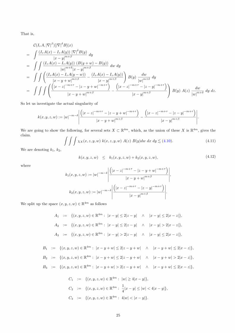
That is,
C(IτA, |∇|β)[|∇|δB](x)
=
ˆ(IτA(x)− IτA(y)) |∇|δB(y)
|x− y|m+βdy
=
ˆ ˆ(IτA(x)− IτA(y)) (B(y + w)−B(y))
|w|m+δ|x− y|m+βdw dy
=
ˆ ˆ ((IτA(x)− IτA(y − w))
|x− y + w|m+β− (IτA(x)− IτA(y))
|x− y|m+β
)B(y)
dw
|w|m+δdy
=
ˆ ˆ ˆ (|x− z|−m+τ − |z − y + w|−m+τ
)|x− y + w|m+β
−
(|x− z|−m+τ − |z − y|−m+τ
)|x− y|m+β
B(y) A(z)dw
|w|m+δdy dz.
So let us investigate the actual singularity of
k(x, y, z, w) := |w|−m−δ∣∣∣∣∣∣(|x− z|−m+τ − |z − y + w|−m+τ
)|x− y + w|m+β
−
(|x− z|−m+τ − |z − y|−m+τ
)|x− y|m+β
∣∣∣∣∣∣.We are going to show the following, for several sets X ⊂ R4m, which, as the union of these X is R4m, gives theclaim. ˆ ˆ ˆ
χX(x, z, y, w) k(x, z, y, w) A(z) B(y)dw dx dy . (4.10). (4.11)
We are denoting k1, k2,
k(x, y, z, w) ≤ k1(x, y, z, w) + k2(x, y, z, w), (4.12)
where
k1(x, y, z, w) := |w|−m−δ∣∣∣∣∣∣(|x− z|−m+τ − |z − y + w|−m+τ
)|x− y + w|m+β
∣∣∣∣∣∣,k2(x, y, z, w) := |w|−m−δ
∣∣∣∣∣∣(|x− z|−m+τ − |z − y|−m+τ
)|x− y|m+β
∣∣∣∣∣∣.We split up the space (x, y, z, w) ∈ R4m as follows
A1 := (x, y, z, w) ∈ R4m : |x− y| ≤ 2|z − y| ∧ |x− y| ≤ 2|x− z|,
A2 := (x, y, z, w) ∈ R4m : |x− y| ≤ 2|z − y| ∧ |x− y| > 2|x− z|,
A3 := (x, y, z, w) ∈ R4m : |x− y| > 2|z − y| ∧ |x− y| ≤ 2|x− z|,
B1 := (x, y, z, w) ∈ R4m : |x− y + w| ≤ 2|z − y + w| ∧ |x− y + w| ≤ 2|x− z|,
B2 := (x, y, z, w) ∈ R4m : |x− y + w| ≤ 2|z − y + w| ∧ |x− y + w| > 2|x− z|,
B3 := (x, y, z, w) ∈ R4m : |x− y + w| > 2|z − y + w| ∧ |x− y + w| ≤ 2|x− z|,
C1 := (x, y, z, w) ∈ R4m : |w| ≥ 4|x− y|,
C2 := (x, y, z, w) ∈ R4m :1
4|x− y| ≤ |w| < 4|x− y|,
C3 := (x, y, z, w) ∈ R4m : 4|w| < |x− y|.
25
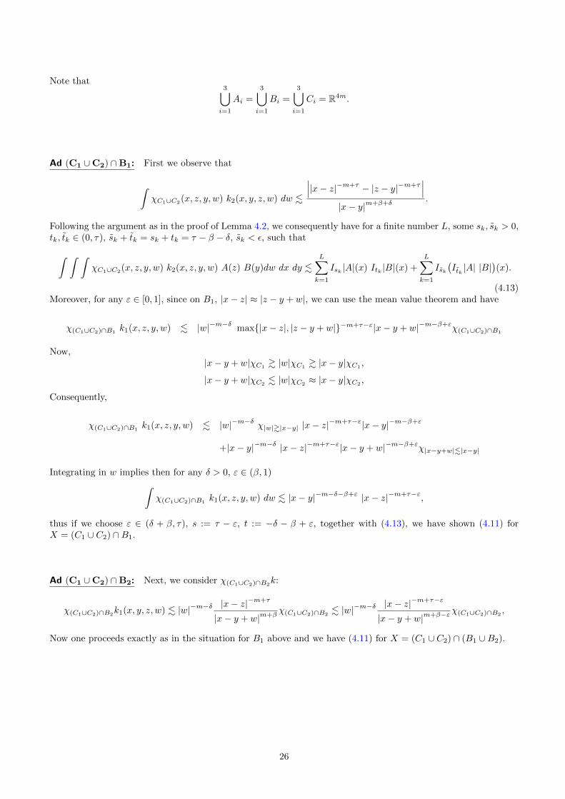
Note that3⋃i=1
Ai =
3⋃i=1
Bi =
3⋃i=1
Ci = R4m.
Ad (C1 ∪C2) ∩B1: First we observe that
ˆχC1∪C2
(x, z, y, w) k2(x, y, z, w) dw .
∣∣∣|x− z|−m+τ − |z − y|−m+τ∣∣∣
|x− y|m+β+δ.
Following the argument as in the proof of Lemma 4.2, we consequently have for a finite number L, some sk, sk > 0,tk, tk ∈ (0, τ), sk + tk = sk + tk = τ − β − δ, sk < ε, such that
ˆ ˆ ˆχC1∪C2(x, z, y, w) k2(x, z, y, w) A(z) B(y)dw dx dy .
L∑k=1
Isk |A|(x) Itk |B|(x) +
L∑k=1
Isk(Itk |A| |B|
)(x).
(4.13)Moreover, for any ε ∈ [0, 1], since on B1, |x− z| ≈ |z − y + w|, we can use the mean value theorem and have
χ(C1∪C2)∩B1k1(x, z, y, w) . |w|−m−δ max|x− z|, |z − y + w|−m+τ−ε|x− y + w|−m−β+ε
χ(C1∪C2)∩B1
Now,|x− y + w|χC1
& |w|χC1& |x− y|χC1
,
|x− y + w|χC2 . |w|χC2 ≈ |x− y|χC2 ,
Consequently,
χ(C1∪C2)∩B1k1(x, z, y, w) . |w|−m−δ χ|w|&|x−y| |x− z|
−m+τ−ε|x− y|−m−β+ε
+|x− y|−m−δ |x− z|−m+τ−ε|x− y + w|−m−β+εχ|x−y+w|.|x−y|
Integrating in w implies then for any δ > 0, ε ∈ (β, 1)
ˆχ(C1∪C2)∩B1
k1(x, z, y, w) dw . |x− y|−m−δ−β+ε |x− z|−m+τ−ε,
thus if we choose ε ∈ (δ + β, τ), s := τ − ε, t := −δ − β + ε, together with (4.13), we have shown (4.11) forX = (C1 ∪ C2) ∩B1.
Ad (C1 ∪C2) ∩B2: Next, we consider χ(C1∪C2)∩B2k:
χ(C1∪C2)∩B2k1(x, y, z, w) . |w|−m−δ |x− z|
−m+τ
|x− y + w|m+βχ(C1∪C2)∩B2
. |w|−m−δ |x− z|−m+τ−ε
|x− y + w|m+β−εχ(C1∪C2)∩B2,
Now one proceeds exactly as in the situation for B1 above and we have (4.11) for X = (C1 ∪ C2) ∩ (B1 ∪B2).
26
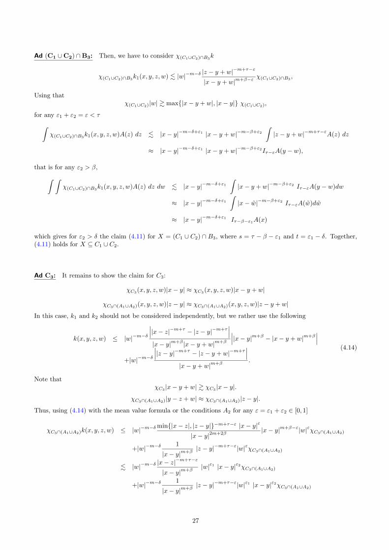
Ad (C1 ∪C2) ∩B3: Then, we have to consider χ(C1∪C2)∩B3k
χ(C1∪C2)∩B3k1(x, y, z, w) . |w|−m−δ |z − y + w|−m+τ−ε
|x− y + w|m+β−ε χ(C1∪C2)∩B3,
Using thatχ(C1∪C2)|w| & max|x− y + w|, |x− y| χ(C1∪C2),
for any ε1 + ε2 = ε < τ
ˆχ(C1∪C2)∩B3
k1(x, y, z, w)A(z) dz . |x− y|−m−δ+ε1 |x− y + w|−m−β+ε2
ˆ|z − y + w|−m+τ−ε
A(z) dz
≈ |x− y|−m−δ+ε1 |x− y + w|−m−β+ε2Iτ−εA(y − w),
that is for any ε2 > β,
ˆ ˆχ(C1∪C2)∩B3
k1(x, y, z, w)A(z) dz dw . |x− y|−m−δ+ε1ˆ|x− y + w|−m−β+ε2 Iτ−εA(y − w)dw
≈ |x− y|−m−δ+ε1ˆ|x− w|−m−β+ε2 Iτ−εA(w)dw
≈ |x− y|−m−δ+ε1 Iτ−β−ε1A(x)
which gives for ε2 > δ the claim (4.11) for X = (C1 ∪ C2) ∩ B3, where s = τ − β − ε1 and t = ε1 − δ. Together,(4.11) holds for X ⊆ C1 ∪ C2.
Ad C3: It remains to show the claim for C3:
χC3(x, y, z, w)|x− y| ≈ χC3(x, y, z, w)|x− y + w|
χC3∩(A1∪A2)(x, y, z, w)|z − y| ≈ χC3∩(A1∪A2)(x, y, z, w)|z − y + w|
In this case, k1 and k2 should not be considered independently, but we rather use the following
k(x, y, z, w) ≤ |w|−m−δ∣∣∣|x− z|−m+τ − |z − y|−m+τ
∣∣∣|x− y|m+β |x− y + w|m+β
∣∣∣|x− y|m+β − |x− y + w|m+β∣∣∣
+|w|−m−δ∣∣∣|z − y|−m+τ − |z − y + w|−m+τ
∣∣∣|x− y + w|m+β
.
(4.14)
Note thatχC3 |x− y + w| & χC3 |x− y|.
χC3∩(A1∪A2)|y − z + w| ≈ χC3∩(A1∪A2)|z − y|.
Thus, using (4.14) with the mean value formula or the conditions A2 for any ε = ε1 + ε2 ∈ [0, 1]
χC3∩(A1∪A2)k(x, y, z, w) ≤ |w|−m−δmin|x− z|, |z − y|−m+τ−ε |x− y|ε
|x− y|2m+2β|x− y|m+β−ε|w|εχC3∩(A1∪A2)
+|w|−m−δ 1
|x− y|m+β|z − y|−m+τ−ε|w|εχC3∩(A1∪A2)
. |w|−m−δ |x− z|−m+τ−ε
|x− y|m+β|w|ε1 |x− y|ε2χC3∩(A1∪A2)
+|w|−m−δ 1
|x− y|m+β|z − y|−m+τ−ε|w|ε1 |x− y|ε2χC3∩(A1∪A2)
27
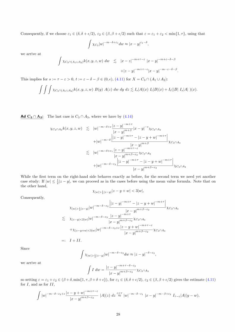
Consequently, if we choose ε1 ∈ (δ, δ + ε/2), ε2 ∈ (β, β + ε/2) such that ε = ε1 + ε2 < min1, τ, using thatˆχC3 |w|
−m−δ+ε1dw ≈ |x− y|ε1−δ,
we arrive at ˆχC3∩(A1∪A2)k(x, y, z, w) dw . |x− z|−m+τ−ε |x− y|−m+ε−δ−β
+|z − y|−m+τ−ε|x− y|−m−ε−δ−β .
This implies for s := τ − ε > 0, t := ε− δ − β ∈ (0, ε), (4.11) for X = C3 ∩ (A1 ∪A2):ˆ ˆ ˆ
χC3∩(A1∪A2)k(x, y, z, w) B(y) A(z) dw dy dz . Is|A|(x) It|B|(x) + It(|B| Is|A| )(x).
Ad C3 ∩A3: The last case is C3 ∩A3, where we have by (4.14)
χC3∩A3k(x, y, z, w) . |w|−m−δ+ε |z − y|
−m+τ
|x− y|m+β|x− y|−εχC3∩A3
+|w|−m−δ∣∣∣|z − y|−m+τ − |z − y + w|−m+τ
∣∣∣|x− y|m+β
χC3∩A3
. |w|−m−δ+ε1 |z − y|−m+τ−ε
|x− y|m+β−ε2 χC3∩A3
+|w|−m−δ−ε2
∣∣∣|z − y|−m+τ − |z − y + w|−m+τ∣∣∣
|x− y|m+β−ε2 χC3∩A3
While the first term on the right-hand side behaves exactly as before, for the second term we need yet anothercase study: If |w| ≤ 1
2 |z − y|, we can proceed as in the cases before using the mean value formula. Note that onthe other hand,
χ|w|> 12 |z−y|
|z − y + w| < 3|w|,
Consequently,
χ|w|> 12 |z−y|
|w|−m−δ−ε2
∣∣∣|z − y|−m+τ − |z − y + w|−m+τ∣∣∣
|x− y|m+β−ε2 χC3∩A3
. χ|z−y|<2|w||w|−m−δ−ε2 |z − y|
−m+τ
|x− y|m+β−ε2 χC3∩A3
+χ|z−y+w|<3|w||w|−m−δ−ε2+ε |z − y + w|−m+τ−ε
|x− y|m+β−ε2 χC3∩A3
=: I + II.
Since ˆχ|w|> 1
2 |z−y||w|−m−δ−ε2dw ≈ |z − y|−δ−ε2 ,
we arrive at ˆI dw =
|z − y|−m+τ−δ−ε2
|x− y|m+β−ε2 χC3∩A3
so setting ε = ε1 + ε2 ∈ (β+ δ,min1, τ, β+ δ+ ε), for ε1 ∈ (δ, δ+ ε/2), ε2 ∈ (β, β+ ε/2) gives the estimate (4.11)for I, and as for II,
ˆ|w|−m−δ−ε2+ε |z − y + w|−m+τ−ε
|x− y|m+β−ε2 |A|(z) dzε<τ≈ |w|−m−δ−ε1 |x− y|−m−β+ε2 Iτ−ε|A|(y − w),
28
ˆ|w|−m−δ−ε2+ε |x− y|−m−β+ε2 Iτ−ε|A|(y − w) dw
ε1>δ≈ |x− y|−m−β+ε2 Iτ−δ−ε2 |A|(y),
and finally, ˆ|x− y|−m−β+ε2 (Iτ−δ−ε2 |A|(y)) |B|(y) dy
ε2>β≈ Iε2−β((Iτ−δ−ε2 |A|) |B|)(x).
Thus, also II has the required estimate and we have shown (4.11) for X = C3 ∩A3.
The following estimate should be compared to the estimates in [Cha82], who extended arguments in [CRW76]from Riesz transforms to Riesz Potentials. Their estimates treat cases in which one of the involved functions bbelongs to BMO, which one usually uses in applications for estimates of that expression in terms of |∇|sb. But ifone knows that |∇|sb exists, then the following estimates are more precise than their BMO-counterparts in termsof Lorentz space estimates.
Lemma 4.6. For any δ > 0 such that s+ δ < 1 and any γ ∈ (s, s+ δ), we have
||∇|sC(a, Is)[b]| ≤ Cs,δ,γ Is+δ−γ
∣∣∣|∇|s+δa∣∣∣ Iγ−s|Isb|+Cs,δ,γ min
Iγ−s
(|Isb| Is+δ−γ
∣∣∣|∇|s+δa∣∣∣), Iγ−s(Is+δ−γ |Isb| ∣∣∣|∇|s+δa∣∣∣)Proof. For δ > 0 such that s+ δ < 1. Set
B := Isb, A := |∇|s+δa.
Then,C(a, Is)[b] = Is((Is+δA)(|∇|sB)− |∇|s((Is+δA)B)).
Now,
|∇|s((Is+δA)B)(x) = cs
ˆ
Rm
Is+δA(x) B(x)− Is+δA(y) B(y)
|x− y|n+s dy
= Is+δA(x) cs
ˆ
Rm
B(x)−B(y)
|x− y|n+s dy + cs
ˆ
Rm
Is+δA(x) − Is+δA(y)
|x− y|n+s B(y) dy
= Is+δA(x) |∇|sB(x) + cs,δ
ˆ
Rm
ˆ
Rm
|z − x|−n+(s+δ) − |z − y|−n+(s+δ)
|x− y|n+s A(z) B(y) dz dy
Let now γ ∈ (s, s+ δ) ⊂ (0, 1) and denote
k(x, y, z) :=|z − x|−n+(s+δ) − |z − y|−n+(s+δ)
|x− y|n+s .
Now we follow the strategy in [Sch11]. We decompose the space (x, y, z) ∈ R3n into several subspaces dependingon the relations of |z − y|, |x− y|, |x− z|:
1 ≤ χ1(x, y, z) + χ2(x, y, z) + χ3(x, y, z) + χ4(x, y, z) for x, y, z ∈ Rm,
whereχ1 := χ|x−y|≤2|z−y| χ|x−y|≤2|x−z|,
χ2 := χ|x−y|≤2|z−y| χ|x−y|>2|x−z|,
χ3 := χ|x−y|>2|z−y| χ|x−y|≤2|x−z| χ|x−z|≤2|z−y|.
χ4 := χ|x−y|>2|z−y| χ|x−y|≤2|x−z| χ|x−z|>2|z−y|.
Then, by the mean value theorem
χ1(x, y, z)k(x, y, z) . |z − x|−n+s+δ−γ |y − x|−n−s+γ .
29
Same holds for
χ2(x, y, z)k(x, y, z) + χ3(x, y, z)k(x, y, z) . |z − x|−n+s+δ−γ |y − x|−n−s+γ .
Finally,χ4(x, y, z)k(x, y, z) . |z − y|−n+s+δ−γ |y − x|−n−s+γ .
Note that
χ4(x, y, z)|x− y| ≤ χ4(x, y, z)|x− z|+ χ4(x, y, z)|z − y| ≤ 3
2χ4(x, y, z)|x− z|,
and
χ4(x, y, z)|x− y| ≥ χ4(x, y, z)|x− z| − χ4(x, y, z)|z − y| ≥ 1
2χ4(x, y, z)|x− z|,
that isχ4(x, y, z)|x− y| ≈ χ4(x, y, z)|x− z|.
That is,χ4(x, y, z)k(x, y, z) . |z − y|−n+s+δ−γ
min|y − x|−n−s+γ , |z − x|−n−s+γ
This implies,
||∇|s((Is+δA)B)(x)− Is+δA(x) |∇|sB(x)|
≤ cs,δ,γ Is+δ−γ |A| Iγ−s|B|+ cs,δ,γ min Iγ−s(|B| Is+δ−γ |A|), Iγ−s(Is+δ−γ |B| |A|) .
It is a simple adaption, to show that in the claim, for both terms on the right-hand side, we could have chosendifferent γ.
For s = 0, a (non-trivial) version of Lemma 4.6, is the following result, for any Riesz transform R. Like Lemma 4.6was related to Chanillo’s [Cha82], this estimate is related to [CRW76]. The proof follows by the same argumentsas the proof of Lemma 4.6, we leave the details to the reader.
Lemma 4.7. Then, for any δ ∈ (0, 1) and any γi ∈ (0, δ), i = 1, 2, we have
|C(a,R)[b]| ≤ CR,δ,γ1 Iδ−γ1
∣∣∣|∇|δa∣∣∣ Iγ1|b|+ CR,δ,γ2
Iγ2
(Iδ−γ2
|b|∣∣∣|∇|δa∣∣∣).
4.3. Fractional product rules in the Hardy-space via para-products – including the limitcase
In this section we introduce several commutators, and show how to use techniques developed by Da Lio andRiviere in [DLR11b] in order to estimate their behavior involving the Hardy spaces H. For the case µ < 1 the newcontribution are the commutators themselves, the techniques for the proof of their behavior follows the argumentsof Da Lio and Riviere. In the case µ = 1, these arguments have to be extended and more precise, in order to showthe same behavior for this limit case, which was unknown up to now. The essential commutator estimate is
‖|∇|µ(R[h] Iµb−R[h Iµb])‖H ≤ ‖h‖2 ‖b‖2 whenever µ ∈ (0, 1]. (4.15)
From this we will conclude‖C(f,R)[|∇|µϕ]‖2 . ‖|∇|µf‖2 [ϕ]BMO, (4.16)
and‖Hµ(ϕ, g)‖2 . ‖|∇|µg‖2 [ϕ]BMO. (4.17)
as well as‖|∇|µHµ(a, b)‖H . ‖|∇|µa‖2 ‖|∇|
µb‖2 for µ ∈ (0, 1]. (4.18)
Note that (4.18) is already known for µ < 1 [DLR11b], and we are going to prove it only for the new situationµ = 1, when we will show that it follows from (4.15).
30
Proof of (4.15). LetT (h, b) := |∇|µ(R[h] Iµb−R[h Iµb])
We will follow the basic ideas of the proof of the commutator theorem in [DLR11b], which goes through withoutgreat changes, if µ < 1, and then point out where it fails if µ = 1. In the latter case, we have make a precisecomputation of the failing term, and show that in fact this term is essentially a commutator as in [CRW76] andanother good term. For a general reference, we refer the reader to the proof in [DLR11b], as we will sketch someof the parts which behave no worse than in their case. In particular, the notion of Besov- and Triebel spaces andtheir respective estimates are taken from [DLR11b] without too much changes.
The para-products and Littlewood-Paley decomposition
We need to control three parts of T . We introduce the projections Π1, Π2, Π3 defined via
Π1T (f, g) :=∑j∈Z
T (fj , gj−4),
Π2T (f, g) :=∑j∈Z
T (f j−4, gj),
Π3T (f, g) :=∑j∈Z
j+4∑l=j−4
T (fj , gl).
Here,supp f∧j ⊂ |ξ| ∈ (2j−1, 2j+1),
andsupp(f j)∧ ⊂ |ξ| ≤ 2j+1.
These terms come from the Littlewood-Paley decomposition. Note that then for k ∈ Z,
Π1T (f, g)k :=
k+3∑j=k−3
T (fj , gj−4)k, (4.19)
Π2T (f, g)k :=
k+3∑j=k−3
T (f j−4, gj)k, (4.20)
Π3T (f, g)k :=
∞∑j=k−5
j+4∑l=j−4
T (fj , gl)k. (4.21)
Estimates from [DLR11b]
Let us recall the following estimates, whose proof up to small adaptions can be found in [DLR11b], for a generaloverview we refer to Tao’s lecture notes [Tao01]: First, denoting with M the maximal function,
supk∈Z
∣∣2−γ |∇|γfk(x)∣∣ .Mf(x) for any γ ≥ 0 and almost every x ∈ Rm. (4.22)
Here, for γ = 0, we set |∇|0 := Id. In fact, for a suitable φ in the Schwartz class,
2−γk|∇|γfk(x) = 2(m−γ)k
ˆφ(2k(x− y)) |∇|γf(y) == 2(m)j
ˆ(|∇|γ φ)(2j(x− y)) f(y).
Now the argument follows the exactly the one of [DLR11b], using that
∣∣∣|∇|γ φ(z)∣∣∣ . 1
1+|z|m+γ if γ > 01
1+|z|β if γ = 0, for any β > 0,
and we arrive at
2−γk|∇|γfk(x) .Mf(x)
∞∑j∈Z
2mj sup|z|≤2j
∣∣∣|∇|γ φ(z)∣∣∣,
31
which is convergent if γ ≥ 0, but might be divergent for γ < 0. This shows (4.22).Let N be a zero-multiplier operator with 0-homogeneous symbol n. We have (cf. [Tao01, Notes 2 for 25A, Lemma1.1])
supk‖2−γkN |∇|γfk‖∞ . CN ‖f‖B0
∞,∞for γ ≥ 0 (4.23)
and thus also‖|∇|γNf j‖∞ . 2γj‖f‖B0
∞,∞for γ > 0 (4.24)
A crucial role is played byˆRm
∑j∈Z
∣∣∣2j(γ−α)N |∇|α−γf j∣∣∣2 1
2
. Cα−γ,N‖f‖2 whenever 0 ≤ γ < α. (4.25)
which follows fromˆRm
∑j∈Z
∣∣∣2j(γ−α)N |∇|α−γf j∣∣∣2 1
2γ<α
. Cα−γ,N
ˆRm
∑j∈Z
∣∣∣2j(γ−α)|∇|α−γfj∣∣∣2 1
2
,
an argument which can be found in the commutator estimates in [DLR11b].
Estimate of Π2
We have
‖Π2T (h, b)‖H . ‖|∇|µΠ2(R[h] Iµb)‖H + ‖R[|∇|µΠ2(h Iµb)]‖H
. ‖|∇|µΠ2(R[h] Iµb)‖H + ‖|∇|µΠ2(h Iµb)‖H.
Let h := R[h] or h, respectively. Then
‖|∇|µΠ2(h Iµb)‖H ≈ ‖|∇|µΠ2(h Iµb)‖F 01,2
≈ ‖Π2(h Iµb)‖Fµ1,2
≈ˆ
Rm
(∑k∈Z
22µk∣∣∣Π2(h Iµb)
∣∣∣2) 12
(4.20)≈
ˆ
Rm
∑k∈Z
22µk
∣∣∣∣∣∣k+3∑j=k−3
(hj−4 Iµbj)k
∣∣∣∣∣∣2
12
.ˆ
Rm
(∑k∈Z
maxj∈[k−3,k+3]∩Z
22µk∣∣∣(hj−4 Iµbj)k
∣∣∣2) 12
.ˆ
Rm
(∑k∈Z
22µk(supi
∣∣∣hi∣∣∣2) |Iµbk|2) 1
2
Thus,
‖|∇|µΠ2(h Iµb)‖H(4.22)
.ˆ
Rm
Mh
(∑k∈Z
22µk|Iµbj |2) 1
2
. ‖h‖2 ‖b‖B02,2
. ‖h‖2 ‖b‖2.
It is worth noting, that this argument holds for any µ > 0.
32
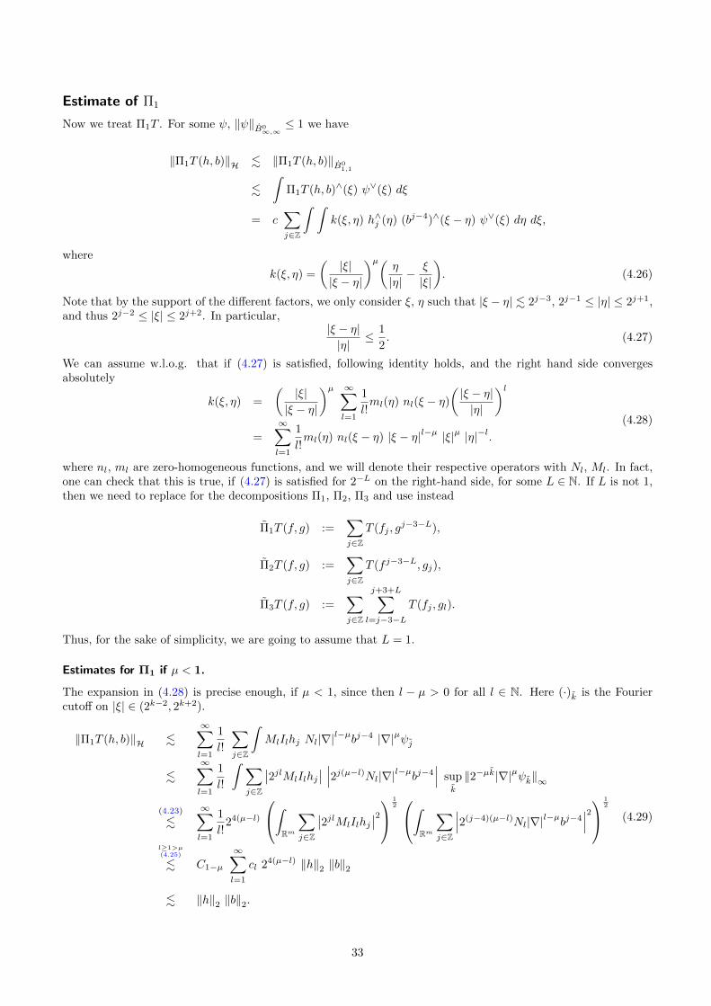
Estimate of Π1
Now we treat Π1T . For some ψ, ‖ψ‖B0∞,∞≤ 1 we have
‖Π1T (h, b)‖H . ‖Π1T (h, b)‖B01,1
.ˆ
Π1T (h, b)∧(ξ) ψ∨(ξ) dξ
= c∑j∈Z
ˆ ˆk(ξ, η) h∧j (η) (bj−4)∧(ξ − η) ψ∨(ξ) dη dξ,
where
k(ξ, η) =
(|ξ||ξ − η|
)µ(η
|η|− ξ
|ξ|
). (4.26)
Note that by the support of the different factors, we only consider ξ, η such that |ξ − η| . 2j−3, 2j−1 ≤ |η| ≤ 2j+1,and thus 2j−2 ≤ |ξ| ≤ 2j+2. In particular,
|ξ − η||η|
≤ 1
2. (4.27)
We can assume w.l.o.g. that if (4.27) is satisfied, following identity holds, and the right hand side convergesabsolutely
k(ξ, η) =
(|ξ||ξ − η|
)µ ∞∑l=1
1
l!ml(η) nl(ξ − η)
(|ξ − η||η|
)l=
∞∑l=1
1
l!ml(η) nl(ξ − η) |ξ − η|l−µ |ξ|µ |η|−l.
(4.28)
where nl, ml are zero-homogeneous functions, and we will denote their respective operators with Nl, Ml. In fact,one can check that this is true, if (4.27) is satisfied for 2−L on the right-hand side, for some L ∈ N. If L is not 1,then we need to replace for the decompositions Π1, Π2, Π3 and use instead
Π1T (f, g) :=∑j∈Z
T (fj , gj−3−L),
Π2T (f, g) :=∑j∈Z
T (f j−3−L, gj),
Π3T (f, g) :=∑j∈Z
j+3+L∑l=j−3−L
T (fj , gl).
Thus, for the sake of simplicity, we are going to assume that L = 1.
Estimates for Π1 if µ < 1.
The expansion in (4.28) is precise enough, if µ < 1, since then l − µ > 0 for all l ∈ N. Here (·)k is the Fouriercutoff on |ξ| ∈ (2k−2, 2k+2).
‖Π1T (h, b)‖H .∞∑l=1
1
l!
∑j∈Z
ˆMlIlhj Nl|∇|l−µbj−4 |∇|µψj
.∞∑l=1
1
l!
ˆ ∑j∈Z
∣∣2jlMlIlhj∣∣ ∣∣∣2j(µ−l)Nl|∇|l−µbj−4
∣∣∣ supk
‖2−µk|∇|µψk‖∞
(4.23)
.∞∑l=1
1
l!24(µ−l)
ˆRm
∑j∈Z
∣∣2jlMlIlhj∣∣2 1
2ˆ
Rm
∑j∈Z
∣∣∣2(j−4)(µ−l)Nl|∇|l−µbj−4∣∣∣2 1
2
l≥1>µ(4.25)
. C1−µ
∞∑l=1
cl 24(µ−l) ‖h‖2 ‖b‖2
. ‖h‖2 ‖b‖2.
(4.29)
33
The crucial point in the above estimate is the application of (4.25), and it was there that we used that µ < l forall l ≥ 1, that is µ < 1. In particular, if the summation on l above had started with l = 2, this estimate wouldhave been true for any µ < 2. Also, note that for µ = 0, this estimate still holds.
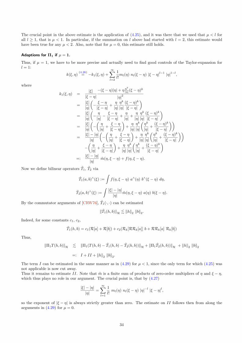
Adaptions for Π1 if µ = 1.
Thus, if µ = 1, we have to be more precise and actually need to find good controls of the Taylor-expansion forl = 1:
k(ξ, η)(4.26)
= −k1(ξ, η) +
∞∑l=2
1
l!ml(η) nl(ξ − η) |ξ − η|l−1 |η|1−l,
where
k1(ξ, η) =|ξ||ξ − η|
−(ξ − η)|η|+ η ηk
|η| (ξ − η)k
|η|2
=|ξ||η|
(− ξ − η|ξ − η|
+η
|η|ηk
|η|(ξ − η)k
|ξ − η|
)=
|ξ||η|
(− η
|η|− ξ − η|ξ − η|
+η
|η|+
η
|η|ηk
|η|(ξ − η)k
|ξ − η|
)=
|ξ||η|
(−(η
|η|+
ξ − η|ξ − η|
)+
η
|η|ηk
|η|
(ηk
|η|+
(ξ − η)k
|ξ − η|
))=
|ξ| − |η||η|
(−(η
|η|+
ξ − η|ξ − η|
)+
η
|η|ηk
|η|
(ηk
|η|+
(ξ − η)k
|ξ − η|
))−(η
|η|+
ξ − η|ξ − η|
)+
η
|η|ηk
|η|
(ηk
|η|+
(ξ − η)k
|ξ − η|
)=:
|ξ| − |η||η|
m(η, ξ − η) + f(η, ξ − η).
Now we define bilinear operators T1, T2 via
T1(a, b)∧(ξ) :=
ˆf(η, ξ − η) a∧(η) b∧(ξ − η) dη,
T2(a, b)∧(ξ) :=
ˆ|ξ| − |η||η|
m(η, ξ − η) a(η) b(ξ − η).
By the commutator arguments of [CRW76], T1(·, ·) can be estimated
‖T1(h, b)‖H . ‖h‖2 ‖b‖2.
Indeed, for some constants c1, c2,
T1(h, b) = c1(R[a] +R[b]) + c2(Rk[RRk[a]] b+RRk[a] Rk[b])
Thus,
‖Π1T (h, b)‖H . ‖Π1(T (h, b)− T1(h, b)− T2(h, b))‖H + ‖Π1T2(h, b))‖H + ‖h‖2 ‖b‖2
=: I + II + ‖h‖2 ‖b‖2.
The term I can be estimated in the same manner as in (4.29) for µ < 1, since the only term for which (4.25) wasnot applicable is now cut away.Thus it remains to estimate II. Note that m is a finite sum of products of zero-order multipliers of η and ξ − η,which thus plays no role in our argument. The crucial point is, that by (4.27)
|ξ| − |η||η|
=
∞∑l=1
1
l!ml(η) nl(ξ − η) |η|−l |ξ − η|l,
so the exponent of |ξ − η| is always strictly greater than zero. The estimate on II follows then from along thearguments in (4.29) for µ = 0.
34
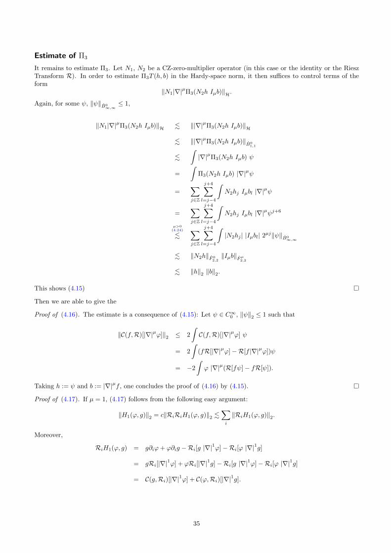
Estimate of Π3
It remains to estimate Π3. Let N1, N2 be a CZ-zero-multiplier operator (in this case or the identity or the RieszTransform R). In order to estimate Π3T (h, b) in the Hardy-space norm, it then suffices to control terms of theform
‖N1|∇|µΠ3(N2h Iµb)‖H.
Again, for some ψ, ‖ψ‖B0∞,∞≤ 1,
‖N1|∇|µΠ3(N2h Iµb)‖H . ‖|∇|µΠ3(N2h Iµb)‖H
. ‖|∇|µΠ3(N2h Iµb)‖B01,1
.ˆ|∇|µΠ3(N2h Iµb) ψ
=
ˆΠ3(N2h Iµb) |∇|µψ
=∑j∈Z
j+4∑l=j−4
ˆN2hj Iµbl |∇|µψ
=∑j∈Z
j+4∑l=j−4
ˆN2hj Iµbl |∇|µψj+6
µ>0(4.24)
.∑j∈Z
j+4∑l=j−4
ˆ|N2hj | |Iµbl| 2µj‖ψ‖B0
∞,∞
. ‖N2h‖F 02,2‖Iµb‖Fµ2,2
. ‖h‖2 ‖b‖2.
This shows (4.15)
Then we are able to give the
Proof of (4.16). The estimate is a consequence of (4.15): Let ψ ∈ C∞0 , ‖ψ‖2 ≤ 1 such that
‖C(f,R)[|∇|µϕ]‖2 ≤ 2
ˆC(f,R)[|∇|µϕ] ψ
= 2
ˆ(fR[|∇|µϕ]−R[f |∇|µϕ])ψ
= −2
ˆϕ |∇|µ(R[fψ]− fR[ψ]).
Taking h := ψ and b := |∇|µf , one concludes the proof of (4.16) by (4.15).
Proof of (4.17). If µ = 1, (4.17) follows from the following easy argument:
‖H1(ϕ, g)‖2 = c‖RiRiH1(ϕ, g)‖2 .∑i
‖RiH1(ϕ, g)‖2.
Moreover,
RiH1(ϕ, g) = g∂iϕ+ ϕ∂ig −Ri[g |∇|1ϕ]−Ri[ϕ |∇|1g]
= gRi[|∇|1ϕ] + ϕRi[|∇|1g]−Ri[g |∇|1ϕ]−Ri[ϕ |∇|1g]
= C(g,Ri)[|∇|1ϕ] + C(ϕ,Ri)[|∇|1g].
35
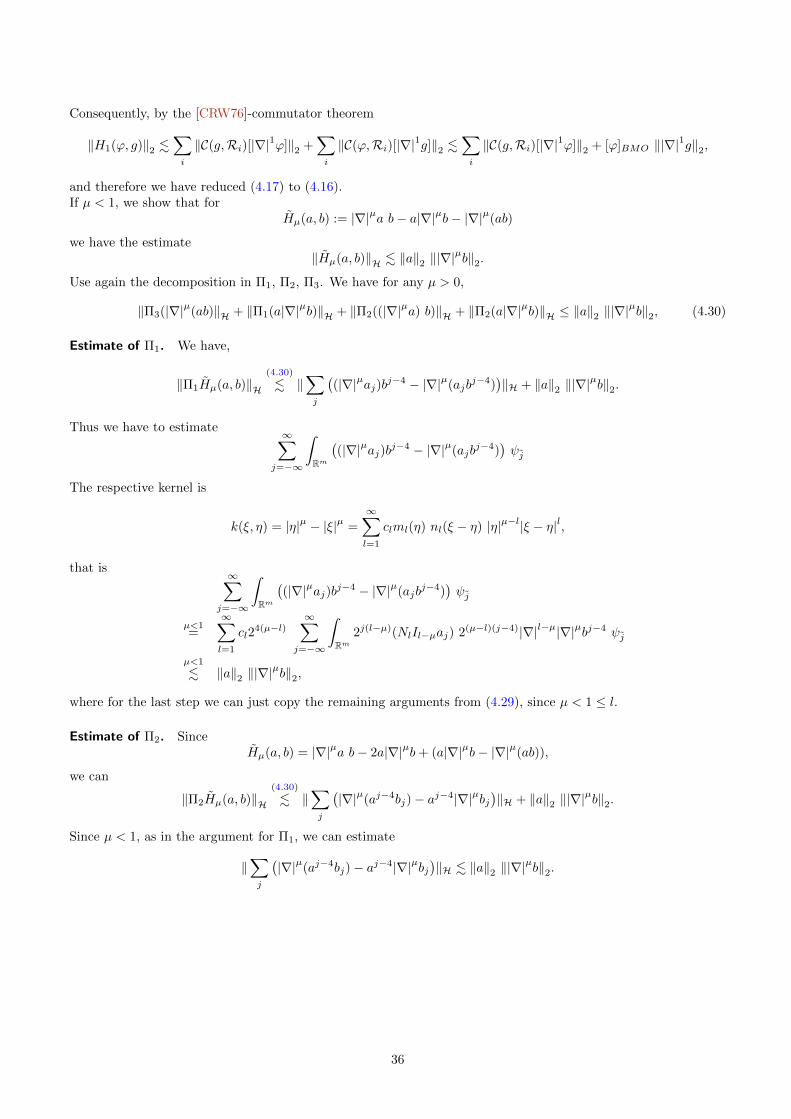
Consequently, by the [CRW76]-commutator theorem
‖H1(ϕ, g)‖2 .∑i
‖C(g,Ri)[|∇|1ϕ]‖2 +∑i
‖C(ϕ,Ri)[|∇|1g]‖2 .∑i
‖C(g,Ri)[|∇|1ϕ]‖2 + [ϕ]BMO ‖|∇|1g‖2,
and therefore we have reduced (4.17) to (4.16).If µ < 1, we show that for
Hµ(a, b) := |∇|µa b− a|∇|µb− |∇|µ(ab)
we have the estimate‖Hµ(a, b)‖H . ‖a‖2 ‖|∇|
µb‖2.
Use again the decomposition in Π1, Π2, Π3. We have for any µ > 0,
‖Π3(|∇|µ(ab)‖H + ‖Π1(a|∇|µb)‖H + ‖Π2((|∇|µa) b)‖H + ‖Π2(a|∇|µb)‖H ≤ ‖a‖2 ‖|∇|µb‖2, (4.30)
Estimate of Π1. We have,
‖Π1Hµ(a, b)‖H(4.30)
. ‖∑j
((|∇|µaj)bj−4 − |∇|µ(ajb
j−4))‖H + ‖a‖2 ‖|∇|
µb‖2.
Thus we have to estimate∞∑
j=−∞
ˆRm
((|∇|µaj)bj−4 − |∇|µ(ajb
j−4))ψj
The respective kernel is
k(ξ, η) = |η|µ − |ξ|µ =
∞∑l=1
clml(η) nl(ξ − η) |η|µ−l|ξ − η|l,
that is∞∑
j=−∞
ˆRm
((|∇|µaj)bj−4 − |∇|µ(ajb
j−4))ψj
µ<1=
∞∑l=1
cl24(µ−l)
∞∑j=−∞
ˆRm
2j(l−µ)(NlIl−µaj) 2(µ−l)(j−4)|∇|l−µ|∇|µbj−4 ψj
µ<1
. ‖a‖2 ‖|∇|µb‖2,
where for the last step we can just copy the remaining arguments from (4.29), since µ < 1 ≤ l.
Estimate of Π2. SinceHµ(a, b) = |∇|µa b− 2a|∇|µb+ (a|∇|µb− |∇|µ(ab)),
we can
‖Π2Hµ(a, b)‖H(4.30)
. ‖∑j
(|∇|µ(aj−4bj)− aj−4|∇|µbj
)‖H + ‖a‖2 ‖|∇|
µb‖2.
Since µ < 1, as in the argument for Π1, we can estimate
‖∑j
(|∇|µ(aj−4bj)− aj−4|∇|µbj
)‖H . ‖a‖2 ‖|∇|
µb‖2.
36
Estimate of Π3. Finally, we have
‖Π3Hµ(a, b)‖H(4.30)
. ‖∑j≈i
(|∇|µ(aj)bi − aj |∇|µbi)‖H + ‖a‖2 ‖|∇|µb‖2,
and have to estimate
∞∑j=−∞
j+4∑i=j−4
(|∇|µ(aj)bi − aj |∇|µbi)ψj−6 +
∞∑j=−∞
j+4∑i=j−4
j+6∑k=j−6
(|∇|µ(aj)bi − aj |∇|µbi)ψk =: I + II,
The kernel here is (note that for ξ ∈ supp(ψj−6)∧, η ∈ supp(aj)∧, |ξ|/|η| ≤ 1
2 which ensures convergence)
k(η, ξ) = |η|µ − |ξ − η|µ =
∞∑l=1
cl ml(ξ − η)nl(ξ)|η|µ−l |ξ|l, (4.31)
thus we have
I =
∞∑l=1
cl
∞∑j=−∞
j+4∑i=j−4
ˆMl|∇|µ−laj bi Nl|∇|lψj−6
.∞∑l=1
cl 2−6l supk
2−l(k−6)‖Nl|∇|lψk−6‖∞∞∑
j=−∞
j+4∑i=j−4
ˆ ∣∣∣2(l−µ)jNl|∇|µ−laj∣∣∣ ∣∣2µibi∣∣
(4.24)
. ‖ψ‖B0∞,∞
∞∑l=1
cl 2−6l∞∑
j=−∞
j+4∑i=j−4
ˆ ∣∣∣2(l−µ)jMl|∇|µ−laj∣∣∣ ∣∣2µibi∣∣
. ‖ψ‖B0∞,∞
‖a‖2 ‖|∇|µb‖2.
For II, where the expansion (4.31) might not be convergent, the situation is even easier,
|II| .∞∑
j=−∞
j+4∑i=j−4
j+6∑k=j−6
ˆ (∣∣2−µj |∇|µaj∣∣ ∣∣2µjbi∣∣+ |aj | ||∇|µbi|)|ψk|
. ‖ψ‖B0∞,∞
ˆ ∑
j
∣∣2−µj |∇|µaj∣∣2 1
2ˆ ∑
j
∣∣2µjbi∣∣2 1
2
+
(ˆ|aj |2
) 12(ˆ||∇|µbi|
2) 1
2
. ‖ψ‖B0
∞,∞‖a‖2 ‖|∇|
µb‖2.
Proof of (4.18) for µ = 1. We have (by the classical product rule, or equivalently expanding the symbols |ξ|2 =
|ξ − η|2 + |η|2 + 2ξ · (ξ − η)). With Rk we will by a abuse of notation call the linear operators with symbol ξk/|ξ|.By the classical product rule for Ri|∇|1 = c∂i
RiH1(a, b) = aRi|∇|1b+ bRi|∇|1a−Ri(a|∇|1b)−Ri(b|∇|1a)
= I1(|∇|1a) Ri|∇|1b+ I1(|∇|1b)Ri|∇|1a−Ri(I1(|∇|1a) |∇|1b)−Ri(I1(|∇|1b) |∇|1a)
= I1(|∇|1a) Ri|∇|1b−Ri(I1(|∇|1a) |∇|1b)
+I1(|∇|1b)Ri|∇|1a−Ri(I1(|∇|1b) |∇|1a)
Thus, Ri|∇|1H1(a, b) can be estimated via (4.15), and as this holds for any i ∈ N, we have (4.18) for µ = 1.
37
5. Energy approach for optimal frame: Proof of Theorem 1.6
In this section we construct a suitable frame P for our equation, transforming the antisymmetric (essentially)L2-potential Ω[] into an L2,1- or even better in an IµH-potential ΩP []. Here, H is the Hardy space, and with theprevious statement we essentially mean that
ˆΩP [f ] ≤ CΩP ‖f‖(2,∞), or
ˆΩP [|∇|µϕ] ≤ CΩP ‖ϕ‖BMO, respectively, (5.1)
where BMO is the space dual to H. This is an improvement, since for the non-transformed Ω, we only had theestimate ˆ
Ω[f ] ≤ CΩ ‖f‖2. (5.2)
For motivation of the arguments presented here, let us recall the classical setting [Riv07], where we have theequation (usually for wi := ∇ui ∈ L2(Rm,R2))
−div(wi) = Ωik · wl,
for Ωik = −Ωki ∈ L2(Rm,R2), and we look for an orthogonal transformation P ∈ W 1,2(Rm, SO(N)), SO(N) ⊂RN×N being the special orthogonal group, such that
ˆΩPik · ∇ϕ = 0, (5.3)
whereΩPij = Pik∇PTkj + PikΩklP
Tlj , or equivalently, − div(Pilw
l) = ΩPik · Pklwl.
Also in this case, the estimate (5.3) is an improvement from the estimate for the non-transformed Ω
ˆΩ · ∇ϕ ≤ CΩ ‖∇ϕ‖2,
philosophically similar to the improvement (5.1) from the starting point (5.2).For the construction of P such that (5.3) holds, there are two different arguments known: Riviere [Riv07] adapteda result by Uhlenbeck [Uhl82] which is based on the continuity method (for the set tΩ, t ∈ [0, 1]) and relies onnon-elementary a-priori estimates for ΩP which also needs L2-smallness of Ω. In [Sch10a] we proposed to usearguments from Helein’s moving frame method [Hel91]: Then the construction of P relies on the fact that (5.3) isthe Euler-Lagrange equation of the energy
E(Q) := ‖ΩQ‖22, Q ∈ SO(N), a.e., (5.4)
the minimizer of which exists by the elementary direct method.Both construction arguments have been generalized to the fractional setting for Ω[] ≡ Ω· a pointwise multiplication-operator [DLR11a, Sch11]. In our situation, where Ω[] is allowed to be a linear bounded operator from L2 to L1,we adapt the argument in [Hel91, Sch10a, Sch11], and minimize essentially the energy
E(Q) := supψ∈L2
ˆΩQ[ψ], Q ∈ SO(N), a.e..
While the construction of a minimizer of E, see Lemma 5.5, is not much more difficult as in the earlier situations[Hel91, Sch10a, Sch11], when computing the Euler-Lagrange equations, see Lemma 5.6, we have several errorterms, which stem from commutators of the form fΩ[g]−Ω[fg], which are trivial if Ω[] is a pointwise-multiplicationoperator Ω[] = Ω·. In Lemma 5.7 we then show that these error terms all behave well enough, if we take the forus relevant case of Ω[] being of the form AR[].
5.1. Preliminary propositions
Here we recall some elementary statements, which enter the proof of Theorem 1.6. Proposition 5.1 and Proposi-tion 5.2 are simple duality arguments for linear, bounded mappings between Banach spaces. Proposition 5.4 is aquantified embedding from L1 into BMO.
38
Proposition 5.1. For any s > 0 there exists Λ0, Cs > 1 such that the following holds: Let f ∈ L2(Rm), |∇|sf ∈L2(Rm) and assume f ≡ 0 on Rm\Br for some Br ⊂ Rm. Then for any Λ ≥ Λ0,
‖|∇|sf‖2,Rm\BΛr≤ Cs Λ−
m2 −s ‖|∇|sf‖2,BΛr
Proof. Using Corollary B.2,
‖|∇|sf‖2,Rm\BΛr. Λ−
m2 −s ‖|∇|sf‖2,Rm\BΛr
+ Λ−m2 −s ‖|∇|sf‖2,BΛr .
Thus, if Λ > Λ0 for a Λ0 depending only on s, we can absorb and conclude.
Proposition 5.2. Let A : L2(Rm) → L1(Rm) be a linear, bounded operator. Then there exists g ∈ L2(Rm),‖g‖2,Rm = 1 such that
sup‖ψ‖2,Rm≤1
ˆA[ψ] =
ˆA[g].
In particular (taking instead of A the operator A := A[χD·], for any D ⊂ Rm there exists gD ∈ L2(D), ‖gD‖2,D ≤ 1,supp g ⊂ D, such that
sup‖ψ‖2,Rm≤1,suppψ⊂D
ˆA[ψ] =
ˆA[gD].
Proof. As f∗ ∈(L2(Rm)
)∗for
f∗(ψ) :=
ˆA[ψ]
is a linear bounded functional, there exists a unique f ∈ L2(Rm) such that
ˆA[ψ] =
ˆfψ, (5.5)
and
‖f‖2,Rm = sup‖ψ‖2,Rm≤1
ˆA[ψ].
On the other hand,
‖f‖22,Rm =
ˆf f
(5.5)=
ˆA[f ],
which in turn implies that for g :=∥∥f∥∥−1
2f ,
sup‖ψ‖2,Rm≤1
ˆA[ψ] = ‖f‖2,Rm =
ˆA[g].
Proposition 5.3. Let A : L2(Rm) → L1(Rm) be a linear, bounded operator. Then there exists a linear, boundedoperator A∗ : L∞(Rm)→ L2(Rm) such that
ˆg A[f ] =
ˆf A∗[g] for any f ∈ L2(Rm), g ∈ L∞(Rm).
Moreover, g = ‖A(1)‖−12 A∗(1) for the g from Proposition 5.2.
Proof. For any g ∈ L∞(Rm), we have
Tg[·] :=
ˆg A[·] ∈
(L2(Rm)
)∗,
thus there exists a unique A∗g ∈ L2(Rm) such that
Tg[f ] =
ˆA∗g f for all f ∈ L2(Rm).
39
For λ1, λ2 ∈ R and g1, g2 ∈ L∞, and any f ∈ L2(Rm)
ˆA∗λ1g1+λ2g2
f = λ1
ˆg1 A[f ] + λ2
ˆg2 A[f ] = λ1
ˆAg1
f + λ2
ˆAg2
f,
which implies that A∗[·] := A∗· is linear. As for boundedness, note that
‖A∗[g]‖2,Rm = sup‖f‖2,Rm≤1
ˆA∗[g]f = sup
‖f‖2,Rm≤1
ˆgA[f ] ≤ ‖g‖∞ ‖A‖L2→L1 ,
that is‖A∗‖L∞→L2 ≤ ‖A‖L2→L1 .
Finally, we have that ˆf ψ
(5.5)=
ˆA[ψ] =
ˆA∗[1] ψ,
which - given that it holds for any ψ ∈ L2(Rm) - implies f = A∗[1].
Proposition 5.4. Let ϕ ∈ C∞0 (Br), then
‖ϕ‖1 ≤ Cm rm [ϕ]BMO.
Proof. Let Λ > 0, then
‖ϕ‖1,Br ≤ ‖ϕ− |BΛr|−1ˆϕ‖
Br
+|Br|BΛr‖ϕ‖1,Br ,
and consequently for, say, Λ = 2,
‖ϕ‖1,Br ≤ 2‖ϕ− |BΛr|−1ˆϕ‖
Br
. (Λr)m |BΛr|−1‖ϕ− |BΛr|−1ˆϕ‖
BΛr
. (Λr)m [ϕ]BMO.
5.2. Energy with potentials
Let Ωi,j : L2(Rm)→ L1(Rm), 1 ≤ i, j ≤ N be a linear bounded Operator. And set
ΩQij [f ] := (|∇|µ(Q− I)ik) QTkj f +QikΩkl[QTljf ],
for supp(Q− I) ⊂ Br, |∇|µQ ∈ L2(RN×N ) and Q ∈ SO(N) almost everywhere. For ψ : Rn → RN×N , we write
ΩQ[ψ] := (|∇|µ(Q− I)ik) QTkj ψij +QikΩkl[QTljψij ],
Having in mind (5.4), we then define the energy
E(Q) ≡ Er,x,Λ,s,2(Q) :=
supψ∈C∞0 (BΛr(x),RN×N )
‖ψ‖2≤1
´Rm
(ΩQ)[ψ] if supp(Q− I) ⊂ Br(x),
∞ else.(5.6)
Obviously, Q ≡ I is admissible and E(I) < ∞. Thus there exists a minimizing sequence, and one can hope for aminimizer:
Lemma 5.5. For any µ > 0 there exists Λ0 > 1 such that for any Λ ≥ Λ0, the following holds: There exists anadmissible function P for E such that E(P ) ≤ E(Q) for any other admissible function Q. Moreover,
‖|∇|µP‖2,BΛr(x) + Λm2 +µ‖|∇|µP‖2,Rm\BΛr(x) ≤ Cµ ‖Ω‖2→1,BΛr(x). (5.7)
Here,‖Ω‖2→1,D := sup
ψ∈C∞0 (D,RN×N ),‖ψ‖2≤1
‖Ω[ψ]‖1
40
Proof. Take Λ0 from Proposition 5.1 and assume Λ ≥ Λ0. We have for any ψ ∈ C∞0 (BΛr,RN×N ), ‖ψ‖2 ≤ 1
E(Q) ≥ˆ
(|∇|µ(Q− I) QT )ijψij +
ˆQΩ[QTψ]
≥ˆ
(|∇|µ(Q− I) QT )ij ψij − ‖Ω‖2→1,BΛr ,
which (taking the supremum over such ψ) implies
‖|∇|µ(Q− I)‖2,BΛr ≤ E(Q) + ‖Ω‖2→1,BΛr .
According to Proposition 5.1, this implies (as Q ≡ I on Rn\Br),
‖|∇|µ(Q− I)‖2,Rm ≤ Cµ (E(Q) + ‖Ω‖2→1,BΛr ).
Consequently, for a minimizing sequence Pk,
‖|∇|µ(Pk − I)‖2,Rm ≤ Cµ ‖Ω‖2→1,BΛr,
and up to taking a subsequence, we may assume that there is an admissible function P such that |∇|µPk convergesL2-weakly to |∇|µP and Pk converges pointwise and strongly to P .Then, for any fixed ψ ∈ C∞0 (BΛr), ‖ψ‖2,RN×N ≤ 1
E(Pk) ≥ˆ
ΩP [ψ] +
ˆΩPk [ψ]− ΩP [ψ].
We claim that ˆΩPk [ψ]− ΩP [ψ]
k→∞−−−−→ 0, (5.8)
which, once proven, implies that
inf E(·) ≥ˆ
ΩPψ,
which by the arbitrary choice of ψ implies that P is a minimizer. In order to show (5.8), note that
ΩPk [ψ]− ΩP [ψ] = |∇|µPk (PTk − PT )ψ + |∇|µ(Pk − P ) PTψ + (Pk − P )Ω[PTk ψ
]+ PΩ
[(PTk − PT )ψ
]=: Ik + IIk + IIIk + IVk.
Since |Pk|, |P | ≤ 1, all terms of the form (PTk −PT )ψk→∞−−−−→ 0 in L2, by Lebesgue’s dominated convergence. Thus,´
Ik +´IVk
k→∞−−−−→ 0. By the weak L2-convergence of |∇|µPk, also´IIk
k→∞−−−−→ 0. Since PTk ψ → PTψ in L2(Rm),
also Ω[PTk ψ
] k→∞−−−−→ Ω[PTψ] in L1 and in particular pointwise almost everywhere. Then also´IIIk
k→∞−−−−→ 0.
Lemma 5.6. Let P be a minimizer of E(·) as in (5.6), and assume that
Ωij [] = −Ωji[] 1 ≤ i, j ≤ N. (5.9)
Then for any ϕ ∈ C∞0 (Br(x)),
−ˆ
ΩP [|∇|µϕ] =1
2
ˆHµ(P − I, PT − I) |∇|µϕ
−ˆso(PC(ϕ,Ω)
[PTΩP
TχDΛ
])
+
ˆso(ΩPχDΛPHµ(ϕ, PT − I))
−ˆso(C(P,Ω)[|∇|µϕ]PT )
+
ˆΩP [(1− χDΛ
)|∇|µϕ].
Here, we denote for a matrix A ∈ RN×N , the antisymmetric part with so(A) = 2−1(A− AT ), and for a mappingg : L2 → L1, we denote g as in Proposition 5.2.
41
Proof. We set D := Br(x) and DΛ := BΛr(x). Let ϕ ∈ C∞0 (D), ω ∈ so(N). We distort the minimizer P of E(·)by
Qε := eεϕωP = P + εϕ ω P + o(ε) ∈ Hn2
I (D,SO(N)),
that is we know thatE(Qε)− E(P ) ≥ 0 (5.10)
We compute
|∇|µ(Qε − I) QT
= |∇|µ(P − I) PT + εϕ(ω |∇|µ(P − I) PT − |∇|µ(P − I) PT ω
)+ ε|∇|µϕ ω + ε ω Hµ(ϕ, P − I)PT + o(ε),
(5.11)and
QεΩ[QTε ·
]= PΩ
[PT ·
]+ ε(ϕ ω PΩ
[PT ·
]− PΩ
[PT ωϕ·
])+ o(ε). (5.12)
Together, we infer from (5.11) and (5.12) (denoting the Hilbert-Schmidt matrix product A : B := AijBij)
ΩQε [ψ] = ΩP [ψ] + ε(ϕω ΩP [ψ]− ΩP [ωψϕ]
)+ ε|∇|µϕ ω : ψ + ε ω Hµ(ϕ, P − I) PT : ψ + o(ε)[ψ].
Thus, for any ε > 0, ψ ∈ C∞0 (DΛ,RN×N ), ‖ψ‖2 ≤ 1,
1
ε(E(Qε)− E(P )) ≥ 1
ε
(ˆΩP [ψ]− E(P )
)+
ˆ (ϕω ΩP [ψ]− ΩP [ωψϕ]
)+
ˆ|∇|µϕ ω : ψ
+
ˆω Hµ(ϕ, P − I) PT : ψ
+o(1).
Let ψ ∈ L2(DΛ) such that E(P ) =´
ΩP [ψ] (cf. Proposition 5.2), this implies for the choice ψ := ψ
0(5.10)
≥ 1
ε(E(Qε)− E(P )) ≥
ˆ (ϕω ΩP [ψ]− ΩP [ωψϕ]
)+
ˆ|∇|µϕ ω : ψ
+
ˆω Hµ(ϕ, P − I) PT : ψ
+o(1).
Letting ε→ 0, we then have
−ˆ|∇|µϕ ω : ψ ≥
ˆϕω ΩP [ψ]− ΩP [ωψϕ]
+
ˆω Hµ(ϕ, P − I) PT : ψ
which holds for any ϕ ∈ C∞0 (Br). Replacing ϕ by −ϕ, we arrive at
−ˆ|∇|µϕ ω : ψ =
ˆϕω ΩP [ψ]− ΩP [ωψϕ] +
ˆω Hµ(ϕ, P − I) PT : ψ. (5.13)
Now we need to be more specific about the characteristics of ψ. We have
E(P ) = supψ
ˆΩP [ψ] = sup
ψ
ˆ|∇|µPik PTkj ψij + PikΩkl[P
Tljψij ].
42
Let Ω∗kl : L∞(Rm)→ L2(Rm) be the linear bounded operator such that (cf. Proposition 5.3)ˆ
Rm
gΩkl[f ] =
ˆ
Rm
Ω∗kl[g] f, for any f ∈ L2(Rm), g ∈ L∞(Rm).
Set then, ((ΩP)∗)
ij[f ] := |∇|µPik PTkjf + Ω∗kl [fPik] PTlj ∈ L2(Rm),
and (ΩP)ij
:=((
ΩP)∗)
ij[1] ∈ L2(Rm).
Since ˆg(ΩP)ij
[f ] =
ˆ ((ΩP)∗)
ij[g] f for all f ∈ L2(Rm), g ∈ L∞(Rm),
we have
E(P ) = supψ
ˆΩP : ψ χDΛ
= c
ˆΩP : ΩP χDΛ
= c
ˆΩP [ΩP χDΛ
],
for some normalizing constant c. That is,
(E(P ))2
=
ˆ (ΩP)ij
[χDΛΩP ij ],
and we can assume ψ = cχDΛΩP = cχDΛ
ΩP for some normalizing constant c. Now,
−ˆ|∇|µϕ ω : ψ = −c
ˆ|∇|µϕ ωijχDΛΩPij = −ωij
ˆΩPij [|∇|
µϕ] +
ˆω : ΩP [(1− χDΛ)|∇|µϕ].
Consequently, (5.13) reads as
−ˆω : ΩP [|∇|µϕ] =
ˆϕωik
(ΩP)kj
[(
ΩP)ijχDΛ
]−(ΩP)ij
[ωik
(ΩP)kjϕ]
+
ˆ
DΛ
ω Hµ(ϕ, P − I) PT : ΩP
+
ˆω : ΩP [(1− χDΛ
)|∇|µϕ].
Note that, since ϕ ∈ C∞0 (Rm) ⊂ L∞,
ωik
ˆ (ΩP)ij
[(
ΩP)kjϕ] = ωik
ˆ (ΩP)ij
(ΩP)kjϕω∈so= 0. (5.14)
By the same argument,
ωik
ˆϕ(ΩP)kj
[χDΛ
(ΩP)ij
] = ωik
ˆϕ(ΩP)kj
[χDΛ
(ΩP)ij
]− ωikˆ (
ΩP)kj
[(
ΩP)ijϕ]
and
ωik
ˆϕ(ΩP)kj
[(
ΩP)ijχDΛ
]
= ωik
ˆ ((ΩP)∗)
kj[ϕ](
ΩP)ijχDΛ
= ωik
ˆϕ((
ΩP)∗)
kj[1](
ΩP)ijχDΛ
− ωikˆ (
ϕ((
ΩP)∗)
kj[1]−
((ΩP)∗)
kj[ϕ]
) (ΩP)ijχDΛ
suppϕ= ωik
ˆϕ((
ΩP)∗)
kj[1](
ΩP)ij− ωik
ˆ (ϕ((
ΩP)∗)
kj[1]−
((ΩP)∗)
kj[ϕ]
) (ΩP)ijχDΛ
(5.14)= 0− ωik
ˆ (ϕ((
ΩP)∗)
kj[1]−
((ΩP)∗)
kj[ϕ]
) (ΩP)ijχDΛ
= ωik
ˆC(ϕ,ΩPkj)[(ΩP )ij χDΛ ],
43
where we denote the commutator CC(b, T )[f ] := b Tf − T (bf).
Thus, we arrive at
−ˆω : so(ΩP [|∇|µϕ])ij = ωik
ˆC(ϕ,(ΩP)kj
)[(
ΩP)ijχDΛ ]
+
ˆω Hµ(ϕ, P − I) PT : ΩPχDΛ
+
ˆω : ΩP [(1− χDΛ
)|∇|µϕ].
One checks, that
C(ϕ,(ΩP)kj
)[(
ΩP)ijχDΛ
] = PklC(ϕ,Ωls
)[PTsj
(ΩP)ijχDΛ
]
Next, (and here the antisymmetry of Ω, (5.9), plays its role)
so(ΩP [|∇|µϕ])ij = so(|∇|µ(P − I) PT )ij |∇|µϕ+1
2PikΩkl[Pjl|∇|µϕ]− 1
2PjkΩkl[Pil|∇|µϕ]
(5.9)= so(|∇|µ(P − I) PT )ij |∇|µϕ+
1
2PikΩkl[Pjl|∇|µϕ] +
1
2PjlΩkl[Pik|∇|µϕ]
= so(|∇|µ(P − I) PT )ij |∇|µϕ+1
2PikΩkl[Pjl|∇|µϕ] +
1
2PjlPikΩkl[|∇|µϕ]
−1
2PjlC(Pik,Ωkl)[|∇|µϕ]
= so(|∇|µ(P − I) PT )ij |∇|µϕ+ PikΩkl[Pjl|∇|µϕ]
+1
2PikC(Pjl,Ωkl)[|∇|µϕ]− 1
2PjlC(Pik,Ωkl)[|∇|µϕ],+
ˆΩP [(1− χDΛ
)|∇|µϕ].
and
so(|∇|µ(P − I) PT ) =1
2|∇|µ(P − I) PT − 1
2P |∇|µ(PT − I)
= |∇|µ(P − I) PT +1
2
(−|∇|µ(P − I) PT − P |∇|µ(PT − I)
)= |∇|µ(P − I) PT +
1
2
(|∇|µ(PPT )− |∇|µ(P − I) PT − P |∇|µ(PT − I)
)= |∇|µ(P − I) PT +
1
2Hµ(P − I, PT − I)
This implies finally (going with ωij ∈ −1, 0, 1 through all the possible matrices with two non-zero entries)
−ˆ
ΩP [|∇|µϕ] =1
2
ˆHµ(P − I, PT − I) |∇|µϕ
+
ˆso(PC(ϕ,Ω)
[PTΩP
TχDΛ
])
+
ˆso(ΩPχDΛPHµ(ϕ, PT − I))
−ˆso(C(P,Ω)[|∇|µϕ]PT )
+
ˆΩP [(1− χDΛ
)|∇|µϕ].
Then, using the commutator estimates in [CRW76], (4.16), (4.17), and (4.18), we have shown the following Lemma,which implies Theorem 1.6
44
Lemma 5.7. Let P be a minimizer of E(·) as in (5.6), Lemma 5.6. Assume moreover, that Ω satisfies (1.6).Then for any ϕ ∈ C∞0 (Br)
−ˆ
ΩP [|∇|µϕ] . Λ−m2 −µ r
m2 −µ ‖A‖2 [ϕ]BMO + ‖A‖22
[ϕ]BMO if µ ∈ (0, 1],
‖|∇|µϕ‖(2,∞) if µ > 1.
Proof. By Lemma 5.5 and Lemma 5.6,
‖ΩP ‖2→1 + ‖ΩP ‖2 + ‖|∇|µP‖2 . ‖Ω[]‖2−>1 . ‖A‖2,
and by Lemma 5.6 we need to estimate
ˆHµ(P − I, PT − I) |∇|µϕ (5.15)
|ˆso(PC(ϕ,Ω)
[PTΩP
TχDΛ
])| . ‖A‖2 ‖C(ϕ,R)
[PTΩP
TχDΛ
])‖
2, (5.16)
|ˆso(ΩPχDΛPHµ(ϕ, PT − I))| . ‖ΩP ‖2 ‖Hµ(ϕ, PT − I)‖2 |, (5.17)
|ˆso(C(P,Ω)[|∇|µϕ]PT )| . ‖A‖2 ‖C(P,R)[|∇|µϕ]‖2 , (5.18)
|ˆ
ΩP [(1− χDΛ)|∇|µϕ]| . ‖ΩP ‖2→1 ‖(1− χDΛ)|∇|µϕ]‖2. (5.19)
The estimate of (5.15) is immediate from (4.18), for the estimate of (5.16) we apply [CRW76]. For the estimateof (5.17) we use (4.17), for (5.18) we have (4.16).It remains to estimate (5.19), which follows from
‖(1− χDΛ)|∇|µϕ]‖2 .∞∑k=1
‖|∇|µϕ‖2,AkΛrL.B.1
.∞∑k=1
(2kΛr)−m2 −µ‖ϕ‖1
P.5.4
.∞∑k=1
(2kΛr)−m2 −µrm [ϕ]BMO.
45
A. Some facts on our fractional operators
The fractional laplacian ∆s2 is usually defined via its Fourier-symbol −|ξ|s. Here, we will mostly use the negative
fractional laplacian (−∆)s2 ≡ |∇|s (which here plays the role of the gradient, or the divergence and rotation in
the classical settings), defined via its symbol |ξ|s. These operators are defined for s ∈ (−m,m), if s < 0, we write∆
s2 ≡ I|s|.
Most of the time, we will use the potential definition: For Schwartz functions f ,
|∇|sf(x) = cs limε→0
ˆ|x−y|>ε
f(x)− f(y)
|x− y|m+s dy for s ∈ (0, 2).
The inverse is the Riesz potential,
Isf(x) = cs limε→0
ˆ|x−y|>ε
f(y)
|x− y|m−sdy for s ∈ (0,m).
We refer, e.g., to [SKM93, Lan72] on hyper-singular operators, generalizations, and different representation for-mulas.Next, we state some useful facts about the fractional laplacian, which we are going to use throughout our paper,as standard repertoire.We have the standard Poincare inequality, for a proof, we refer, e.g., to [Sch10b].
Lemma A.1 (Poincare inequality with compact support). Let s ∈ [0,m), p ∈ (1,∞), q ∈ [1,∞], then for anyBr ⊂ Rm, and any f ∈ C∞0 (Br)
‖f‖(p1,q1) ≤ Cs rs‖|∇|sf‖(p1,q1).
The (scaling invatiant) Sobolev inequality takes the form
Lemma A.2 (Sobolev inequality). Let s ∈ [0,m), p1, p2 ∈ [1,∞), q ∈ [1,∞], for any f ∈ S(Rm),
‖f‖(p1,q)≤ ‖|∇|sf‖(p2,q)
,
where1
p2=
1
p1+
s
m.
For p1 =∞, we have the following limiting version of Sobolev’s inequality:
Lemma A.3 (Limiting Sobolev inequality). Let s ∈ (0,m). For any f ∈ S(Rm),
‖f‖∞ ≤ ‖|∇|sf‖(ms ,1),
Also, we have the following Holder-like inequality
Lemma A.4 (Holder inequality). Let s ∈ [0,m), then for any p1 < p2, for any Br ⊂ Rm, and any f ∈ C∞0 (Br)
‖|∇|sf‖(p1,q1) ≤ Cs,p1,p2rmp1− mp2 ‖|∇|sf‖(p2,∞)
Proof. Let Λ > 2, then‖|∇|sf‖(p1,q1),BΛr
. Cs,p1,p2,Λ rmp1− mp2 ‖|∇|sf‖(p2,∞).
On the other hand, for some θ > 0, by Lemma B.1, Lemma A.1,
‖|∇|sf‖(p1,q1),Rn\BΛr. Λ−θr−s‖f‖(p1,q1) . Λ−θ‖|∇|sf‖(p1,q1).
For sufficiently large Λ we can absorb the latter term into the left-hand side, and obtain the claim.
From the Lemmata before, we also have
Lemma A.5 (Poincare-Sobolev inequality with compact support). Let s ∈ (0,m), p1, q1 ∈ (1,∞), then we haves ≤ t, for any Br ⊂ Rm, and any f ∈ C∞0 (Br)
‖|∇|sf‖(p1,q1) ≤ Cp1,q1,p2,q2,s,t rmp1− mp2
+s−t ‖|∇|tf‖(p2,q2),
where p2 ∈ (1,∞) such that1
p2≤ 1
p1+s− tm
and q2 =∞ if the above inequality is strict, else q1 = q2.
46
A very important ingredient in our arguments is the boundedness of the Riesz potential on Morrey spaces.
Lemma A.6 ([Ada75]). Let s ∈ [0,m), p1, p2 ∈ (1,∞), q ∈ [1,∞], λ ∈ (0,m], such that
1
p1=
1
p2− s
λ.
Then for any f ∈ S(Rm),‖Isf‖(p1,q)λ
. ‖Isf‖(p2,q)λ.
The following is an easy equivalence result, recall (1.17).
Proposition A.7. Let Λ > 2, σ > 0. Then,
∞∑k=K0
2−kσ ‖f‖(p,q),Akr ≤ Cσ‖f‖(p,q),BΛr+
∞∑k=0
2−kσ ‖f‖(p,q),AkΛr
Proof. Let k0 := blog2 Λc ≥ 1, then2k0 ≤ Λ < 2k0+1
We have2−σ(l+k0)‖f‖(p,q),Ak
2l+k0r
. 2−σk02−σ(l−1)‖f‖(p,q),Ak2l−1Λr
+ 2−σk0 2σl‖f‖(p,q),Ak2lΛr
.
47
B. Quasi-locality
In this section we gather some facts which quantify the quasi-local behaviour of operators like fractional laplacians|∇|α, Riesz transforms R, and Riesz potentials Is. With “quasi-local” we mean the following: Let A ⊂ Rm besome domain and assume that supp f ⊂ A. If we take T to be any of the above mentioned operators, then thereis no reason why suppTf ⊂ A, nor suppTf ⊂ BδA for some δ > 0. Nevertheless, if we take a domain B ⊂ Rm,dist(A,B) > ε > 0, then Tf ∈ C∞(B). In fact, in this case
Tf(x) = k ∗ f(x) for x ∈ B,
where k is a kernel of the form k(y) = h(y/|y|) |y|−n−s for some s ∈ (−m,m), h some smooth function on Sm−1.Since supp f ⊂ A and x ∈ B, we can replace
Tf(x) = k ∗ f(x),
where k(y) = (1 − η(y))k(y), and η ∈ C∞0 (Bε(0)), η ≡ 1 on Bε/2(0). Obviously, k ∈ C∞(Rm), and consequentlyso is Tf . In fact, by the usual Young-inequality, we have
‖Tf‖∞,B ≤ ‖k‖∞ ‖f‖1 ≤ ‖k‖∞,Rm\Bε/2(0) ‖f‖1 ≤ C‖h‖∞ ε−n−s ‖f‖1.
That is, although we cannot ensure that Tf ≡ 0 in B (as it would be, e.g., the case for local operators like ∇), wecan at least quantify that the farer away B is from A, the less is the norm of Tf on B. In particular, we have
Lemma B.1 (Quasi-locality (I)). Let p1, p2, q1, q2 ∈ [1,∞], s ∈ (−m,m) and Ω1,Ω2 ⊂ Rm be disjoint domainswith d := dist(Ω1,Ω2) > 0 and with positive and finite Lebesgue measure. Then, for any f ∈ S(R),
‖∆ s2 (fχΩ2)‖(p1,q1),Ω1
≤ d−m−s|Ω1|1/p1 |Ω2|1−1/p2‖f‖(p2,q2),Ω2,
where we set
∆s2 :=
|∇|s if s > 0,
Id or R if s = 0,
I|s| if s < 0.
Often we will use the above also for Ω1 or Ω2 to be a complement of some ball Br. This is valid, since Rm\Br =⋃∞k=1A
kr , recall (1.17). Then
χRm\Br =
∞∑k=1
χAkr ,
and for each Akr we have the correct estimate, so that for s ∈ (−m,m) the sum on k is convergent. Consequently,as a special case, using also Poincare inequality (cf. Section A), we have
Corollary B.2 (Quasi-locality (II)). Let p1, p2 ∈ (1,∞), q1, q2 ∈ [1,∞], s, t ∈ [0,m). Then, for any Br ⊂ Rm,f ∈ S(R), Λ > 1, whenever
‖|∇|s(fχBr )‖(p1,q1),Rm\BΛr≤ Cs,p1,p2,q1Λ−m−s+
mp1 r
mp1− mp2−s+t‖|∇|t(χBrf)‖(p2,q2),Br .
Lemma B.3 (Quasilocality (III)). Let f, g ∈ S(Rm), Ω1,Ω2 ⊂ Rm be disjoint domains with d := dist(Ω1,Ω2) > 0and with positive and finite Lebesgue measure.
‖|∇|s((∆ t2 fχΩ1
)gχΩ2)‖(p1,q1) . sup
α∈[0,s]
d−m−t−α ‖fχΩ1‖1 ‖||∇|
s−α(gχΩ2
)|‖(p1,q1)
for any t ∈ (−m,m), s ∈ (0,m).
Proof. By the disjoint support, pointwise almost everywhere,
(∆t2 fχΩ1
) gχΩ2(x) = c
ˆ|x− y|−m−tf(y)χΩ1
(y) g(x)χΩ2(x) dy.
Let η ≡ η ∈ C∞([0,∞)), η ≡ 1 on [1,∞), η ≡ 0 on [0, 1], and set
Kt,d(z) := |z|−m−t η(z/d) ∈ Lp(Rm) ∩ L∞(Rm) ∩ C∞(Rm) for any p > max mm+t , 1.
48
It is worth noting the scaling behaviour of Kt,d in d,
Kt,d(z) = d−m−tKt,1(z/d). (B.1)
We have(∆
t2 fχΩ1
) gχΩ2= (Kt,d ∗ fχΩ1
) gχΩ2.
Now we know that|∇|sKt,d ∈ C∞(Rm),
and on the other hand||∇|sKt,d(x)| . Cd |x|−m−s−t,
so together|∇|sKt,d ∈ Lp(Rm) ∩ L∞(Rm) ∩ C∞(Rm), for any p > max m
m+t+s , 1.
By the scaling (B.1), we also know the exact dependence on d:
‖|∇|αKt,d‖(p,q) = d−m−t−α+mp ‖|∇|αKt,1‖(p,q)
Consequently,‖|∇|s(Kt,d ∗ fχΩ1)‖∞ . ‖fχΩ1‖1.
Then our product rule, Lemma 4.2, tells us that we essentially have to estimate
‖|∇|s((|∇|tfχΩ1)gχΩ2
)‖(p1,q1)
. supα∈[0,s]
‖||∇|αKt,d ∗ fχΩ1| ||∇|s−α(gχΩ2
)|‖(p1,q1)
. supα∈[0,s]
‖||∇|αKt,d ∗ fχΩ1|‖∞ ‖||∇|
s−α(gχΩ2
)|‖(p1,q1)
. supα∈[0,s]
‖|∇|αKt,d‖∞‖fχΩ1‖1 ‖||∇|
s−α(gχΩ2
)|‖(p1,q1)
. supα∈[0,s]
d−m−t−α ‖fχΩ1‖1 ‖||∇|
s−α(gχΩ2
)|‖(p1,q1).
49
C. Left-hand side estimates
Lemma C.1 (Left-hand side estimates). For a uniform constant C, and any κ ∈ [µ, 2µ), µ ≤ m2 , Λ ≥ 4,
‖v‖( mm−κ ,∞),BΛ−1r
≤ C supϕ∈C∞0 (Br,RN )
1
‖|∇|τϕ‖( mτ+κ−µ ,1)
ˆv · |∇|µϕ
+C Λκ−m ‖v‖( mm−κ ,∞),Br
+C Λκ−m∞∑k=0
2k(κ−m) ‖v‖( mm−κ ,∞),B
Akr
.
More generally, for α ∈ (0, µ],
‖|∇|µ−αv‖( mm+µ−α−κ ,∞),BΛ−1r
≤ C supϕ∈C∞0 (Br,RN )
1
‖|∇|αϕ‖( mα+κ−µ ,1)
ˆv · |∇|µϕ
+C Λκ−m+α−µ ‖v‖( mm−κ ,∞),Br
+C Λκ−m+α−µ∞∑k=0
2k(κ−m+α−µ) ‖v‖( mm−κ ,∞),Akr
.
Proof. Let f ∈ C∞0 (BΛ−1r,RN ), ‖f‖( mα+κ−µ ,1) ≤ 1 such that
‖|∇|µ−αv‖( mm+µ−α−κ ,∞),BΛ−1r
≤ 2
ˆ|∇|µ−αv · f.
Decompose for the usual cutoff ηr/2 ∈ C∞0 (B r2),
f = |∇|α(η r2Iαf) + |∇|α((1− η r
2)Iαf) =: |∇|αg1 + |∇|αg2.
As usual, using Lemma 4.1 (for β = 0) as an approximate product rule, for finitely many sk ∈ [0, α],
‖|∇|αg1‖( mα+κ−µ ,1) .
∑k
‖Isk∣∣|∇|αη r
2
∣∣‖( mα−sk
,∞)‖Iα−sk |f |‖( m
sk+κ−µ ,1) . ‖f‖p.
As for g2, for a usual decomposition unity ηl ∈ C∞0 (B2lr\B2l−2r)
|∇|αg2 =
∞∑l=−2
|∇|α(ηlIαf) =:
∞∑l=−2
|∇|αgl
and with the help of Lemma B.3,
‖|∇|µgl‖(mκ ,1) . (2lΛ)κ−m−µ+α ‖f‖ mα+κ−µ
≤ (2lΛ)κ−m+α−µ‖f‖ mα+κ−µ
,
and for k ≥ 1,‖|∇|µgl‖(mκ ,1),B
2kr\B
2k−1r. Λκ−m+α−µ 2kκ+maxk,l(−m−µ)+lα ‖f‖ m
α+κ−µ.
Consequently, for any k ∈ N0,
‖|∇|µg2‖(mκ ,1),Akr. (2kΛ)κ−m+α−µ ‖f‖ m
α+κ−µ.
So we conclude using
ˆv · |∇|µg2 . ‖v‖( m
m−κ ,∞),Br‖|∇|µg2‖(mκ ,1),Br
+
∞∑k=1
‖v‖( mm−κ ,∞),Akr
‖|∇|µg2‖(mκ ,1),Akr
50
D. Iteration
Lemma D.1. Let q ∈ (0, 1), K > 1, ε > 0 and assume
ε+ q2K +Kε1
1− q≤ 1
16. (D.1)
Let moreover ψ,Φ : (0,∞)→ (0,∞), ψ ≤ Φ, and Φ monotone rising. Assume that for all λ ∈ (0, 1]
Φ(2−Kλ
)≤ ε Φ(λ) + ε
∞∑k=0
qk ψ(2kλ). (D.2)
If there is G <∞ so that for all λ ∈ (0, 1)∞∑k=0
qk ψ(2kλ) ≤ G.
Then, for all λ ∈ (0, 1),
Φ(λ) ≤ 32 λ1
2K (Φ(1) +G).
For a proof, we refer, e.g., to the arxiv-version of [Sch11], or [BRS12].
References
[Ada75] D. R. Adams. A note on Riesz potentials. Duke Math. J., 42(4):765–778, 1975.
[BRS12] S. Blatt, P. Reiter, and A. Schikorra. Fine analysis of critical knots - stationary points of the Mobiusenergy are smooth. Preprint, 2012.
[Cha82] S. Chanillo. A note on commutators. Indiana Univ. Math. J., 31(1):7–16, 1982.
[CRW76] R. R. Coifman, R. Rochberg, and G. Weiss. Factorization theorems for Hardy spaces in several variables.Ann. of Math. (2), 103(3):611–635, 1976.
[DL10] F. Da Lio. Fractional Harmonic Maps into Manifolds in odd dimension n > 1. Preprint,arXiv:1012.2741, 2010.
[DLR11a] F. Da Lio and T. Riviere. Sub-criticality of non-local Schrodinger systems with antisymmetric potentialsand applications to half-harmonic maps. Advances in Mathematics, 227(3):1300 – 1348, 2011.
[DLR11b] F. Da Lio and T. Riviere. Three-term commutator estimates and the regularity of 1/2-harmonic mapsinto spheres. Analysis and PDE, 4(1):149 – 190, 2011.
[DLS12a] F. Da Lio and A. Schikorra. n/p-harmonic maps: regularity for the sphere case. Preprint,arXiv:1202.1151, 2012.
[DLS12b] F. Da Lio and A. Schikorra. n/p-harmonic maps: the manifold case. in preparation, 2012.
[Fre73] J. Frehse. A discontinuous solution of a mildly nonlinear elliptic system. Math. Z., 134:229–230, 1973.
[FS72] C. Fefferman and E. M. Stein. Hp spaces of several variables. Acta Math., 129(3-4): 137–193, 1972.
[Gra08] L. Grafakos. Classical Fourier analysis (Second Ed.). Springer, Berlin, 2008.
[Gru84] M Gruter. Conformally invariant variational integrals and the removability of isolated singularities.Manuscripta Math., 47:85–104, 1984.
[Hel91] F. Helein. Regularite des applications faiblement harmoniques entre une surface et une variete rieman-nienne. C.R. Acad. Sci. Paris 312, Serie I, pages 591–596, 1991.
[Hun66] R. Hunt. On L(p, q) Spaces. L’Enseignement Mathematique, Vol. 12, pages 249 – 276, 1966.
[KP88] T. Kato and G. Ponce. Commutator estimates and the Euler and Navier-Stokes equations. Comm.Pure Appl. Math., 41(7):891–907, 1988.
51
[Lan72] N. S. Landkof. Foundations of modern potential theory. Springer, Berlin, 1972.
[Riv07] T. Riviere. Conservation laws for conformally invariant variational problems. Invent. Math., 168(1):1–22, 2007.
[RS08] T. Riviere and M. Struwe. Partial regularity for harmonic maps and related problems. Comm. PureAppl. Math., 61(4):451–463, 2008.
[Sch10a] A. Schikorra. A Remark on Gauge Transformations and the Moving Frame Method.Ann.Inst.H.Poincare, 27:503–515, 2010.
[Sch10b] A. Schikorra. Regularity of n/2-harmonic maps into spheres. PhD-Thesis, arXiv:1003.0646v1, 2010.
[Sch11] A. Schikorra. Interior and Boundary-Regularity of Fractional Harmonic Maps on Domains. Preprint,arXiv:1103.5203, 2011.
[Sch12] A. Schikorra. Regularity of n/2-harmonic maps into spheres. J. Differential Equations, 252:1862–1911,2012.
[Sem94] S. Semmes. A primer on Hardy spaces, and some remarks on a theorem of Evans and Muller. Com-mun. Partial Differ. Equations, 19(1-2): 277–319, 1994.
[Sha12] B. Sharp. Higher integrability for solutions to a system of critical elliptic PDE. Preprint,arXiv:1112.1127, 2012.
[SKM93] S. Samko, A. Kilbas, and O. Marichev. Fractional integrals and derivatives. Gordon and Breach SciencePublishers, Yverdon, 1993.
[ST11] B. Sharp and P. Topping. Decay estimates for Riviere’s equation, with applications to regularity andcompactness. Preprint, arXiv:1102.0713, 2011.
[Ste93] E. M. Stein. Harmonic analysis: Real-variable methods, orthogonality, and oscillatory integrals. Withthe assistance of Timothy S. Murphy, volume 43 of Princeton Mathematical Series. Princeton UniversityPress, Princeton, NJ, 1993.
[Str08] M. Struwe. Partial regularity for biharmonic maps, revisited. Calc. Var. Partial Differential Equations,33(2):249–262, 2008.
[Tao01] T. Tao. Harmonic analysis in the phase plane. Lecture Notes, http://www.math.ucla.edu/~tao/
254a.1.01w/. 2001.
[Tar85] L. Tartar. Remarks on oscillations and Stokes’ equation. In Macroscopic modelling of turbulent flows(Nice, 1984), volume 230 of Lecture Notes in Phys., pages 24–31. Springer, Berlin, 1985.
[Tar07] L. Tartar. An introduction to Sobolev spaces and interpolation spaces, volume 3 of Lecture Notes of theUnione Matematica Italiana. Springer, Berlin, 2007.
[Uhl82] K. K. Uhlenbeck. Connections with Lp bounds on curvature. Commun. Math. Phys., 83(1): 31–42,1982.
52