ΠΑΝΕΠΙΣΤΗΜΙΟ ΘΕΣΣΑΛΙΑΣ

ΠΟΛΥΤΕΧΝΙΚΗ ΣΧΟΛΗ

ΤΜΗΜΑ ΜΗΧΑΝΟΛΟΓΩΝ ΜΗΧΑΝΙΚΩΝ ΒΙΟΜΗΧΑΝΙΑΣ

Διατριβή

ΒΕΛΤΙΣΤΟΠΟΙΗΣΗ ΠΡΟΓΡΑΜΜΑΤΙΣΜΟΥ ΠΑΡΑΓΩΓΗΣ ΚΑΙ

ΔΙΑΝΟΜΗΣ ΠΡΟΪΟΝΤΩΝ ΣΕ ΧΗΜΙΚΗ ΒΙΟΜΗΧΑΝΙΑ

ΡΗΤΙΝΗΣ PET

υπό

ΟΛΥΜΠΙΑΣ ΧΑΤΖΗΚΩΝΣΤΑΝΤΙΝΟΥ

Διπλωματούχου Μηχανολόγου και Αεροναυπηγού Μηχανικού Πανεπιστημίου Πατρών, 2005 Μ.Δ.Ε. Μηχανολόγου Μηχανικού Πανεπιστημίου Θεσσαλίας, 2009

Υπεβλήθη για την εκπλήρωση μέρους των

απαιτήσεων για την απόκτηση του

Διδακτορικού Διπλώματος

2009

ii

© 2009 Ολυμπία Χατζηκωνσταντίνου

Η έγκριση της διδακτορικής διατριβής από το Τμήμα Μηχανολόγων Μηχανικών της Πολυτεχνικής

Σχολής του Πανεπιστημίου Θεσσαλίας δεν υποδηλώνει αποδοχή των απόψεων του συγγραφέα (Ν.

5343/32 αρ. 202 παρ. 2).

iii

Εγκρίθηκε από τα Μέλη της Επταμελούς Εξεταστικής Επιτροπής:

Πρώτος Εξεταστής (Επιβλέπων Καθηγητής) Δρ. Γεώργιος Λυμπερόπουλος, Καθηγητής Τμήματος Μηχανολόγων Μηχανικών Πανεπιστημίου Θεσσαλίας

Δεύτερος Εξεταστής (μέλος Συμβουλευτικής Επιτροπής)

Δρ. Αθανάσιος Ζηλιασκόπουλος, Καθηγητής Τμήματος Μηχανολόγων Μηχανικών Πανεπιστημίου Θεσσαλίας

Τρίτος Εξεταστής (μέλος Συμβουλευτικής Επιτροπής)

Δρ. Γεώργιος Ταγαράς, Καθηγητής Τμήματος Μηχανολόγων Μηχανικών Αριστοτελείου Πανεπιστημίου Θεσσαλονίκης

Τέταρτος Εξεταστής

Δρ. Δημήτριος Παντελής, Επίκουρος Καθηγητής Τμήματος Μηχανολόγων Μηχανικών Πανεπιστημίου Θεσσαλίας

Πέμπτος Εξεταστής

Δρ. Γεώργιος Κοζανίδης, Λέκτορας Τμήματος Μηχανολόγων Μηχανικών Πανεπιστημίου Θεσσαλίας

Έκτος Εξεταστής

Δρ. Μιχαήλ Γεωργιάδης, Αναπληρωτής Καθηγητής Τμήματος Μηχανικών Πληροφορικής και Τηλεπικοινωνιών Πανεπιστημίου Δυτικής Μακεδονίας

Έβδομος Εξεταστής

Δρ. Αιμιλία Κονδύλη, Αναπληρώτρια Καθηγήτρια Τμήματος Μηχανολογίας Τεχνολογικού Εκπαιδευτικού Ιδρύματος Πειραιά

iv

Ευχαριστίες

Καταρχάς, θέλω να ευχαριστήσω τον επιβλέποντα της διδακτορικής διατριβής μου, Καθηγητή κ.

Γεώργιο Λυμπερόπουλο, για την πολύτιμη καθοδήγηση και επίβλεψη της διατριβής μου. Επίσης,

ευχαριστώ τα υπόλοιπα μέλη της εξεταστικής επιτροπής της διατριβής μου, Καθηγητές κκ.

Αθανάσιο Ζηλιασκόπουλο, Γεώργιο Ταγαρά, Δημήτριο Παντελή, Γεώργιο Κοζανίδη, Μιχαήλ

Γεωργιάδη και Αιμιλία Κονδύλη, για την προσεκτική ανάγνωση της εργασίας μου και για τις

χρήσιμες υποδείξεις τους. Ιδιαίτερες ευχαριστίες οφείλω στους Καθηγητές κ. Κοζανίδη και κ.

Παντελή για την σημαντική καθοδήγησή τους στις δύο βασικές ενότητες της διατριβής μου που

παρουσιάζονται στα Κεφάλαια 2 και 3, αντίστοιχα. Ακόμα, ευχαριστώ θερμά όλους τους φίλους

και συνεργάτες μου και ιδιαίτερα τον Ευστράτιο Αθανασίου που με βοήθησαν και με υποστήριξαν

κατά την διάρκεια της εκπόνησης της διατριβής μου. Πάνω από όλα, είμαι ευγνώμων στους γονείς

μου, Δημήτρη και Αριστέα Χατζηκωνσταντίνου και στην αδερφή μου Μαρία, για την ολόψυχη

υποστήριξή τους όλα τα χρόνια των σπουδών μου. Τους αφιερώνω τη διδακτορική διατριβή μου.

Η εκπόνηση της παρούσας διατριβής υποστηρίχθηκε οικονομικά από το έργο «03ΕΔ913 –

Βελτιστοποίηση προγραμματισμού παραγωγής και διανομής προϊόντων σε χημική βιομηχανία

παραγωγής ρητίνης PET» που συγχρηματοδοτήθηκε από πόρους του δημόσιου (85%) και ιδιωτικού

τομέα (15%) στο πλαίσιο της Πράξης ΠΕΝΕΔ 2003 του Μέτρου 8.3 του Επιχειρησιακού

Προγράμματος «Ανταγωνιστικότητα» του Γ’ Κοινοτικού Πλαισίου Στήριξης. Το 75% της

δημόσιας δαπάνης προήλθε από την Ευρωπαϊκή Ένωση (Ευρωπαϊκό Κοινοτικό Ταμείο) και το

25% από το Ελληνικό Δημόσιο (Υπουργείο Ανάπτυξης: Γενική Γραμματεία Έρευνας και

Τεχνολογίας). Η ιδιωτική δαπάνη προήλθε εξ’ ολοκλήρου από την βιομηχανία Artenius Hellas,

S.A., PET Industry, μέλους του ομίλου βιομηχανιών συσκευασιών PET, La Seda de Barcelona.

Θέλω να ευχαριστήσω τον Διευθυντή του εργοστασίου της Artenius Hellas, κ. Δημήτριο Φιλίππου,

και τους συνεργάτες του, για την πολύτιμη καθοδήγησή τους, ιδιαίτερα στα αρχικά στάδια της

διατριβής, που με μύησε στις λεπτομέρειες ενός πραγματικού προβλήματος της βιομηχανίας το

οποίο απετέλεσε κίνητρο για την ανάπτυξη των προτύπων και μεθοδολογιών που παρουσιάζονται

στην διατριβή.

Ολυμπία Χατζηκωνσταντίνου

v

ΒΕΛΤΙΣΤΟΠΟΙΗΣΗ ΠΡΟΓΡΑΜΜΑΤΙΣΜΟΥ ΠΑΡΑΓΩΓΗΣ ΚΑΙ

ΔΙΑΝΟΜΗΣ ΠΡΟΪΟΝΤΩΝ ΣΕ ΧΗΜΙΚΗ ΒΙΟΜΗΧΑΝΙΑ

ΡΗΤΙΝΗΣ PET

ΟΛΥΜΠΙΑ ΧΑΤΖΗΚΩΣΤΑΝΤΙΝΟΥ

Πανεπιστήμιο Θεσσαλίας, Πολυτεχνική Σχολή, Τμήμα Μηχανολόγων Μηχανικών, 2009

Επιβλέπων Καθηγητής: Δρ. Γεώργιος Λυμπερόπουλος, Καθηγητής Στοχαστικών Μεθόδων στη

Διοίκηση Παραγωγής

Περίληψη

Το κίνητρο της διδακτορικής διατριβής προήλθε από την ανάγκη βελτιστοποίησης του

προγραμματισμού παραγωγής σε μια πραγματική χημική βιομηχανία παραγωγής ρητίνης PET. Η

ανάγκη αυτή οδήγησε στην ανάπτυξη δύο διαφορετικών μαθηματικών μοντέλων που

αντιμετωπίζουν το πρόβλημα του προγραμματισμού παραγωγής στη συγκεκριμένη βιομηχανία

αλλά και σε άλλες με παρεμφερή χαρακτηριστικά, σε δύο διαφορετικά επίπεδα. Ο βασικός κορμός

της διδακτορικής διατριβής αποτελείται από δύο βασικές ενότητες, στις οποίες παρουσιάζεται η

μορφοποίηση, ανάλυση και επίλυση των δύο αυτών μοντέλων, αντίστοιχα.

Στην πρώτη ενότητα που καταλαμβάνει το Κεφάλαιο 2, αναπτύσσεται ένα μοντέλο Μεικτού

Ακέραιου Γραμμικού Προγραμματισμού (Mixed Integer Linear Programming ή MILP) για τον

χρονικό προγραμματισμό της παραγωγής μιας μονάδας συνεχούς ροής που παράγει διαφορετικές

ποιότητες (grades) ρητίνης PET. Ο χρόνος στο μοντέλο είναι διακριτοποιημένος. Ο αντικειμενικός

vi

στόχος είναι να ελαχιστοποιηθεί το κόστος που σχετίζεται με τις αλλαγές ρύθμισης (setup

changeovers) της παραγωγής από μία ποιότητα προϊόντος σε μια άλλη, ούτως ώστε να

αποφευχθούν ανεπιθύμητες μεταβολές στις ιδιότητες του παραγόμενου προϊόντος που λαμβάνουν

χώρα κατά την διάρκεια τέτοιων αλλαγών. Οι περιορισμοί του μοντέλου αφορούν, μεταξύ άλλων,

την σειρά των αλλαγών ρύθμισης παραγωγής, την σειριακή παραγωγή με περιορισμένη

παραγωγική δυναμικότητα και περιορισμένη χωρητικότητα, την μικτή και ευέλικτη πεπερασμένη

χωρητικότητα αποθηκών ενδιάμεσων και τελικών προϊόντων, τις απαιτήσεις ικανοποίησης της

ζήτησης σε ενδιάμεσες ημερομηνίες (και όχι μόνον στο τέλος του ορίζοντα προγραμματισμού), κ.α.

Παρουσιάζεται μια μελέτη περίπτωσης που καταδεικνύει πώς μπορεί να εφαρμοστεί το μοντέλο σε

ένα πραγματικό σενάριο και οδηγεί στην εξαγωγή χρήσιμων συμπερασμάτων και ενόρασης όσον

αφορά στην συμπεριφορά του μοντέλου. Η εμπειρία από τα αριθμητικά παραδείγματα δείχνει ότι οι

υπολογιστικές απαιτήσεις για την επίλυση του μοντέλου είναι λογικές για μεγέθη προβλημάτων

που απαντώνται σε πρακτικές εφαρμογές.

Το μοντέλο βελτιστοποίησης του προγραμματισμού της παραγωγής που παρουσιάζεται

στην πρώτη ενότητας της διατριβής είναι ένα κλασικό καθοριστικό μοντέλο διακριτού χρόνου και

πεπερασμένου χρονικού ορίζοντα. Περιγράφει με μεγάλη ακρίβεια το πραγματικό πρόβλημα

προγραμματισμού παραγωγής σε έναν βραχύ χρονικό ορίζοντα (τυπικά, μια εβδομάδα), όπου η

ζήτηση των διαφορετικών ποιοτήτων θεωρείται γνωστή. Όμως, επειδή στο πραγματικό σύστημα, η

παραγωγή και η ζήτηση συνεχίζονται και μετά το πέρας του ορίζοντα προγραμματισμού, το

πρόγραμμα παραγωγής είναι λογικό να μην επιτρέπει στο απόθεμα των προϊόντων να πέσει κάτω

από κάποιο απόθεμα ασφαλείας, ούτως ώστε να μπορεί να αντιμετωπισθεί η αβέβαιη ζήτηση και

μετά το πέρας του χρονικού ορίζοντα προγραμματισμού. Για τον αποτελεσματικό σχεδιασμό των

αποθεμάτων ασφαλείας απαιτείται μια πιο μακροσκοπική ανάλυση που να περιγράφει το σύστημα

vii

με λιγότερη λεπτομέρεια, αλλά να λαμβάνει ρητά υπόψη την στοχαστική φύση της ζήτησης. Μια

τέτοια ανάλυση αποτελεί το αντικείμενο της δεύτερης ενότητας της διδακτορικής διατριβής.

Συγκεκριμένα, στη δεύτερη ενότητα που καταλαμβάνει το Κεφάλαιο 3, αναπτύσσεται ένα

μαθηματικό μοντέλο μιας παραλλαγής του Στοχαστικού Προβλήματος του Βέλτιστου Χρονικού

Προγραμματισμού Παρτίδων Παραγωγής (Stochastic Economic Lot Scheduling Problem ή

SELSP), στο οποίο μια μονάδα συνεχούς παραγωγής πρέπει να παράγει διαφορετικές ποιότητες

μιας οικογένειας προϊόντων για να ικανοποιήσει τυχαία αλλά στάσιμα κατανεμημένη ζήτηση για

κάθε ποιότητα από μια κοινή αποθήκη τελικών προϊόντων με περιορισμένη χωρητικότητα. Η

ζήτηση που δεν μπορεί να ικανοποιηθεί από το απόθεμα, χάνεται. Η πρώτη ύλη είναι πάντα

διαθέσιμη, και η μονάδα παραγωγής παράγει συνεχώς και με σταθερό ρυθμό. Όταν η μονάδα είναι

ρυθμισμένη να παράγει μια συγκεκριμένη ποιότητα, οι μόνες επιτρεπτές αλλαγές είναι από αυτή

την ποιότητα στην αμέσως χαμηλότερη ή υψηλότερη ποιότητα. Όλοι οι χρόνοι αλλαγών είναι

σταθεροί και ίδιοι. Υπάρχει ένα κόστος αλλαγής ανά περίσταση αλλαγής, ένα κόστος υπερχείλισης

ανά μονάδα πλεονασματικού προϊόντος οποτεδήποτε δεν υπάρχει αρκετός χώρος στην αποθήκη

τελικών προϊόντων για να αποθηκευτεί το παραγόμενο προϊόν, και ένα κόστος χαμένων πωλήσεων

ανά μονάδα ελλειμματικού προϊόντος οποτεδήποτε δεν υπάρχει αρκετό απόθεμα τελικών

προϊόντων για να ικανοποιηθεί η ζήτηση. Μοντελοποιούμε το SELSP ως μια Μαρκοβιανή

Διαδικασία Αποφάσεων (Markov Decision Process ή MDP) διακριτού χρόνου, όπου σε κάθε περίοδο η

απόφαση είναι αν θα ξεκινήσει μια αλλαγή ρύθμισης προς μια γειτονική ποιότητα προϊόντος ή αν θα

παραμείνει η ρύθμιση της μονάδας παραγωγής ως έχει, βάσει της τρέχουσας κατάστασης του συστήματος

που ορίζεται από την τρέχουσα ρύθμιση της μονάδας και τα επίπεδα αποθεμάτων τελικών προϊόντων όλων

των ποιοτήτων. Ο στόχος είναι να ελαχιστοποιηθεί το μακροχρόνιο (απείρου ορίζοντα) προσδοκώμενο μέσο

κόστος ανά περίοδο. Για προβλήματα 2 και 3 ποιοτήτων προϊόντος επιλύουμε αριθμητικά το ακριβές

πρόβλημα MDP χρησιμοποιώντας την μέθοδο των διαδοχικών προσεγγίσεων του διαφορικού κόστους. Για

προβλήματα με περισσότερες από 3 ποιότητες προϊόντος αναπτύσσουμε μια ευρετική διαδικασία επίλυσης

viii

που βασίζεται στην προσέγγιση του αρχικού προβλήματος των πολλαπλών ποιοτήτων από πολλά

υποπροβλήματα 3 ποιοτήτων που επιλύονται με την μέθοδο των διαδοχικών προσεγγίσεων. Παρουσιάζουμε

αριθμητικά αποτελέσματα για παραδείγματα προβλημάτων 2-5 ποιοτήτων. Για τα παραδείγματα των 2 και 3

ποιοτήτων χρησιμοποιούμε την ακριβή μέθοδο επίλυσης για να αποκτήσουμε ενόραση όσον αφορά στη

δομή της βέλτιστης πολιτικής αλλαγών ρύθμισης. Για τα παραδείγματα των 4 και 5 ποιοτήτων συγκρίνουμε

την απόδοση της ευρετικής διαδικασίας επίλυσης σε σχέση με αυτήν της ακριβούς μεθόδου.

UNIVERSITY OF THESSALY

SCHOOL OF ENGINEERING

DEPARTMENT OF MECHANICAL ENGINEERING

Dissertation

PRODUCTION SCHEDULING OPTIMIZATION IN A PET RESIN

CHEMICAL INDUSTRY

by

OLYMPIA HATZIKONSTANTINOU

Diploma in Mechanical & Aeronautical Engineering, University of Patras, 2005 Postgraduate Specialization Diploma in Mechanical Engineering, University of Thessaly, 2009

Submitted in partial fulfillment of the

requirements for the degree of

Doctor of Philosophy

2009

ii

© 2009 Olympia Hatzikonstantinou

The approval of this Ph.D. Dissertation by the Department of Mechanical Engineering of the School

of Engineering of the University of Thessaly does not imply acceptance of the writer’s opinions.

(Law 5343/32, article 202 par. 2).

iii

Approved by the Members of the Examination Committee:

First Reader (Advisor) Dr. George Liberopoulos, Professor, Department of Mechanical Engineering, University of Thessaly

Second Reader (member of Advisory Committee)

Dr. Athanassios Ziliaskopoulos, Professor, Department of Mechanical Engineering, University of Thessaly

Third Reader (member of Advisory Committee)

Dr. George Tagaras, Professor, Department of Mechanical Engineering, Aristotle University of Thessaloniki

Fourth Reader

Dr. Dimitrios Pandelis, Assistant Professor, Department of Mechanical Engineering, University of Thessaly

Fifth Reader

Dr. George Kozanidis, Lecturer, Department of Mechanical Engineering, University of Thessaly

Sixth Reader

Dr. Michael Georgiadis, Associate Professor, Department of Computer and Telecommunications Engineering, University of Western Macedonia

Seventh Reader

Dr. Emilia Kondili, Associate Professor, Department of Mechanical Technology, Technical Educational Institute of Piraeus

iv

Acknowledgements

First and foremost, I want to thank my dissertation advisor, Professor George Liberopoulos, for his

valuable guidance and supervision of my dissertation. I also thank the other members of the

examination committee of my dissertation, Professors Athanasios Ziliaskopoulos, George Tagaras,

Dimitrios Pandelis, George Kozanidis, Michael Georgiadis and Emilia Kodili, for carefully reading

my dissertation and making useful suggestions. I owe special thanks to Professors Kozanidis and

Pandelis for guiding me through the two main parts of my dissertation, which are presented in

Chapters 2 and 3, respectively. In addition, I thank all my friends and colleagues, especially

Efstatios Athanasiou, who helped and supported me during my PhD work. Above all, I am indebted

to my parents, Dimitris and Aristea Hatzikonstantinou and my sister Maria, for their unconditional

support throughout all the years of my studies. I dedicate this dissertation to them.

The work presented in this dissertation was supported by grant “03Δ913 – Optimization of

production scheduling and product distribution in a chemical plant producing PET resin,” which

was co-financed by the public (85%) and private (15%) sector within the Action “PENED 2003” of

Measure 8.3 of the Operational Program “Competitiveness” of the third European Community

Support Framework. 75% of the public funding came from the European Union (European

Community Fund) and 25% came from the Greek Public Sector (Ministry of Development –

General Secretariat of Research and Technology). All private funding came from Artenius Hellas,

S.A., PET Industry, which is a member of the group La Seda de Barcelona, that specializes in PET

industrial packaging. I want to thank the plant manager, Mr. Dimitris Filippou, and his colleagues

for their valuable guidance, especially at the early stages of my dissertation, which introduced me

into the details of a real industrial problem that motivated the development of the models and

solution methodologies presented in my dissertation.

Olympia Hatzikonstantinou

v

PRODUCTION SCHEDULING OPTIMIZATION IN A PET

RESIN CHEMICAL INDUSTRY

OLYMPIA HATZIKONSTANTINOU

University of Thessaly, School of Engineering, Department of Mechanical Engineering, 2009

Dissertation Supervisor: Dr. George Liberopoulos, Professor of Production Management

Abstract

The motivation for this dissertation originated form the need to optimize the scheduling of

production in a real PET resin plant. This need led to the development of two different

mathematical models that address the production scheduling problem in the particular industry that

motivated this study as well as in similar industries at two different levels. The main body of the

dissertation is divided into two parts in which we present the formulation, analysis and solution of

each of the two models, respectively.

In the first part, which occupies Chapter 2, we develop a discrete-time, Mixed Integer Linear

Programming (MILP) model for the production scheduling of a continuous-process multi-grade

PET resin plant. The objective is to minimize the cost associated with grade changeovers in order to

avoid undesirable variations in base resin properties and process conditions that occur during such

changes. The constraints of the model include requirements related to sequence-dependent

changeovers, sequential processing with production and space capacity, mixed and flexible finite

intermediate storage, and intermediate demand due-dates. We present a case study that illustrates

the application of the model on a real problem scenario and provides insight into its behavior. The

vi

numerical experience demonstrates that the computational requirements of the model are quite

reasonable for problem sizes that typically arise in practical applications.

The production scheduling optimization model that is presented in the first part of this

dissertation, is a typical deterministic, discrete-time, finite-horizon optimization model. It describes

in great detail and accuracy the real production scheduling problem in the short term (typically one

week), where the demand for the different grades is considered to be known. In real life, however,

production and demand continue after the end of the scheduling horizon. With this in mind, it is

reasonable to design the production schedule in such a way that the finished goods inventory at the

end of the scheduling horizon does not fall below a certain safety stock level, so that the unknown

random demand after the end of the scheduling horizon can be met. To effectively design such

safety stock levels for each grade, it is necessary to perform a more macroscopic analysis which

describes the system in less detail but takes into account the stochastic nature of demand. Such an

analysis is performed in the second part of this dissertation.

More specifically, in the second part, which occupies Chapter 3, we study a variant of the

Stochastic Economic Lot Scheduling Problem (SELSP) in which a single production facility must

produce several different grades of a family of products to meet random stationary demand for each

grade from a common Finished-Goods (FG) inventory buffer with limited storage capacity.

Demand that can not be satisfied directly from inventory is lost. Raw material is always available,

and the production facility continuously produces at a constant rate. When the facility is set up to

produce a particular grade, the only allowable changeovers are from that grade to the next lower or

higher grade. All changeover times are constant and equal to each other. There is a changeover cost

per changeover occasion, a spill-over cost per unit of product in excess whenever there is not

enough space in the FG buffer to store the produced grade, and a lost-sales cost per unit short

whenever there is not enough FG inventory to satisfy the demand. We model the SELSP as a

vii

discrete-time Markov Decision Process (MDP), where in each time period the decision is whether

to initiate a changeover to a neighboring grade or keep the set up of the production facility

unchanged, based on the current state of the system which is defined by the current set up of the

facility and the FG inventory levels of all the grades. The goal is to minimize the (long-run)

expected average cost per period. For 2- and 3-grade problems, we numerically solve the exact

MDP problem using the value iteration method. For problems with more than three grades, we

develop a heuristic solution procedure which is based on approximating the original multi-grade

problem by several 3-grade sub-problems and numerically solving each sub-problem using value

iteration. We present numerical results for problem examples with 2-5 grades. For the 2- and 3-

grade examples, we use the exact solution procedure to obtain insights into the structure of the

optimal changeover policy. For the 4- and 5-grade examples, we compare the performance of the

heuristic solution procedure against that of the exact procedure.

viii

ix

Contents

Chapter 1 Introduction................................................................................................................... 1 1.1 Motivation and background ................................................................................................................... 1 1.2 Literature review..................................................................................................................................... 3 1.3 Dissertation organization...................................................................................................................... 12 Chapter 2 Production scheduling of a multi-grade PET resin plant ....................................... 15 2.1 Operation of a PET plant ..................................................................................................................... 16 2.2 MILP model development .................................................................................................................... 23 2.3 Application of the model ....................................................................................................................... 37 2.3.1 Computation of safety stock levels...................................................................................................... 39 2.3.2 Numerical results ................................................................................................................................. 43 2.3.3 Computational experience ................................................................................................................... 49 2.4 Conclusions ............................................................................................................................................ 55 Chapter 3 The stochastic economic lot sizing problem for continuous nonstop multi-grade

production ................................................................................................................... 57 3.1 Introduction ........................................................................................................................................... 58 3.2 Problem formulation and dynamic programming solution............................................................... 62 3.3 Heuristic solution procedure ................................................................................................................ 65 3.4 Numerical results................................................................................................................................... 69 3.4.1 2-grade example .................................................................................................................................. 70 3.4.2 3-grade example .................................................................................................................................. 77 3.4.3 4-grade and 5-grade examples ............................................................................................................. 82 3.5 Conclusions ............................................................................................................................................ 86 Chapter 4 Dissertation summary ................................................................................................ 89

Bibliography ..................................................................................................................................... 93 Appendix A: Demand data used in the MILP model application presented in Section 2.3 ................................... 101 Appendix B: Single 2-week MILP problem results vs. two 1-week MILP problem results for the MILP model

application presented in Section 2.3................................................................................................... 105 Appendix C: AMPL codes for the MILP problem developed in Section 2.2........................................................... 109 Appendix D: Matlab codes for implementing the exact and heuristic solution procedures developed in

Sections 3.2 and 3.3.............................................................................................................................. 117 Appendix E: Results of the heuristic policy evaluated in Section 3.4.3 for different values of parameter α ........ 135

x

xi

List of Tables Table 2-1. Grade of final product based on color and IV combination ............................................. 17

Table 2-2. Sample mean and standard deviation of the daily demand for each grade and demand

type............................................................................................................................................. 39

Table 2-3. Optimal safety stock level of grade j, when the facility is set up to produce grade i,

Imin,i,j ........................................................................................................................................... 41

Table 2-4. Mean daily demand, E[dj], market share, pj, and safety stock level, Imin,j, for each

grade j......................................................................................................................................... 41

Table 2-5. Fraction of the demand requested from the LFSS silos and the warehouse, and safety

stock level in the LFSS silos and the warehouse, for each grade j ............................................ 42

Table 2-6. Safety stocks at the LFSS and the warehouse, and initial quantities in the warehouse.... 43

Table 2-7. Number of binary decision variables................................................................................ 50

Table 2-8. Number of continuous decision variables ........................................................................ 50

Table 2-9. Number of constraints ...................................................................................................... 51

Table 2-10. Optimal cost (number of changeovers) and CPU time for each of the 24 runs of the

numerical example presented in Section 2.3.............................................................................. 52

Table 2-11. Effect of increasing the length of the scheduling horizon .............................................. 53

Table 3-1. Probability distribution of demand, Pr(Dn=i), for the 2-grade example........................... 70

Table 3-2. Results for the 2-grade example ....................................................................................... 71

Table 3-3. Optimal policy μ*(s, R) for the 2-grade example.............................................................. 73

Table 3-4. Description of bottle-grade PET resin final products....................................................... 77

Table 3-5. Probability distribution of demand, Pr(Dn=i), for the 3-grade example........................... 78

Table 3-6. Optimal policy μ*(s, R) for the 3-grade example.............................................................. 79

Table 3-7. Optimal target inventory level, xn*(s), for the 3-grade example....................................... 81

Table 3-8. Probability distribution of demand, Pr(Dj = i), for the 4-grade and 5-grade examples .... 82

Table 3-9. Results for the 4-grade example ....................................................................................... 84

Table 3-10. Results for the 5-grade example ..................................................................................... 86

Table A-1. Daily demand values for 6 months used in the example solved in Section 2.3............. 101

Table A-2. Optimal cost (number of changeovers) and CPU time for each of the 100 instances of

the numerical example presented in Section 2.3, where we solved the scheduling problem

for weeks 5 and 6 as a single 2-week MILP problem and as two sequential 1-week MILP

problems, respectively ............................................................................................................. 105

xii

Table A-3. Complete set of results of the heuristic policy evaluated using the value iteration

method for the 4-grade example presented in Section 3.4.3.................................................... 135

Table A-4. Complete set of results of the heuristic policy evaluated using simulation for the 4-

grade example presented in Section 3.4.3................................................................................ 136

Table A-5. Complete set of results of the heuristic policy evaluated using simulation for the 5-

grade example presented in Section 3.4.3................................................................................ 137

xiii

List of Figures

Figure 2-1. Material flow in a PET resin production plant................................................................ 19

Figure 2-2. Time shift representation in the production process ....................................................... 30

Figure 2-3. Evolution of the final grade produced in each period ..................................................... 43

Figure 2-4. Evolution of inventory level in silos 1-4 of the LFSS at the end of each week.............. 44

Figure 2-5. Evolution of inventory level in silos 5-8 of the LFSS at the end of each week.............. 45

Figure 2-6. Evolution of inventory level in the warehouse at the end of each week......................... 45

Figure 2-7. Evolution of inventory level in silos 1-4 of the LFSS at the end of each period in

week 5 ........................................................................................................................................ 46

Figure 2-8. Evolution of inventory level in silos 5-8 of the LFSS at the end of each period in

week 5 ........................................................................................................................................ 47

Figure 2-9. Evolution of inventory level in the warehouse at the end of each period in week 5....... 47

Figure 2-10. Scheduled demand per grade and type for each period in week 5 ................................ 48

Figure 2-11. Color setting at POLY, IV setting at SSP and final grade produced in each period of

week 5 ........................................................................................................................................ 49

Figure 3-1. Optimal changeover policy for cases 2 (left) and 4 (right) of Table 3-2, for X = 40 ...... 74

Figure 3-2. Optimal changeover policy for case 3 (left) and case 1 (right) of Table 3-2, for X = 80 76

Figure 3-3. Optimal changeover policy for x2 = 90 (left) and x2 = 70 (right), for the 3-grade

example ...................................................................................................................................... 80

Figure 3-4. Optimal changeover policy for x2 = 30 (left) and x2 = 10 (right), for the 3-grade

example ...................................................................................................................................... 80

Figure 3-5. Expected average cost per period of the heuristic, Jh(α), vs. α, for the 4-grade

example ...................................................................................................................................... 85

Figure 3-6. Expected average cost per period of the heuristic, Jh(α), vs. α, for the 5-grade

example ...................................................................................................................................... 86

xiv

1

Chapter 1 Introduction

In this chapter, we provide some background information which supports the motivation behind this

dissertation. We also review the relevant literature, and we give a brief description of the two main

parts of the dissertation, which occupy Chapters 2 and 3, respectively.

1.1 Motivation and background

Chemicals and plastics production is based on the processing of oil, natural gas and coal. It starts

from a few main organic monomer chemical groupings, such as ethylene and propylene, from

which various polymers are produced. A handful of these polymers form the inputs into

manufactured intermediate and final plastic products. Although polymerization occurs via a variety

of reaction mechanisms with different degrees of complexity, the industrial production of most

polymers is more or less the same, from an operations management point of view. More

specifically, it is common for polymerization plants to operate in a continuous manner in which

several grades are produced using the same equipment. In this context, grades are understood as

products made from the same polymer but with different end use properties, such as brightness,

color, mechanical strength, etc. These end use properties of grades are dependent on molecular

weight distribution and monomer conversion, which in turn are determined by operating conditions.

Transition times in grade polymerization plants can be long, resulting in a considerable amount of

off-specifications production. As such, the number of transitions to be made during a production

2

sequence is an important aspect to consider when determining a production schedule for

polymerization plants (Terrazas-Moreno et al. 2007).

One of the most important classes of polymers in use today is polyesters, which contain the

ester functional group in their main chain. The widespread uses of polyesters range from bottles for

carbonated soft drinks and water to fibers for shirts and other apparel. Polyesters also form the basis

for photographic film and recording tape. Although there are many polyesters, the term “polyester”

as a specific material most commonly refers to Polyethylene Terephthalate (PET), which is the

workhorse polyester used for packaging, stretch-blown bottles and for the production of fiber of

textile products. In this thisis, we focus on the production scheduling of bottle-grade PET. The

scheduling paradigm that we develop for PET, however, is representative of the entire polymer

production industry, because it has similar characteristics from an operations management point of

view, as was mentioned above.

PET is an inert plastic that does not leach harmful materials into its contents, when used as a

container. For this reason, it has been the main solution for the production of packaging containers

for over 20 years. The US Food and Drug Administration (FDA) has done rigorous testing to ensure

that PET containers are safe and suitable for food and beverage storage and use. As a result, PET

has been widely used for the production of food and beverage containers. An additional advantage

of PET containers is that they are 100% recyclable and extremely light. Thus, they help diminish

the formation of packaging waste and reduce the emission of contaminants during their transport.

Furthermore, since they require less fuel during transportation, they also help saving energy.

According to McGehee et al. (2004), the key factors that increase the cost of production in a

PET plant are: 1) insufficient equipment utilization, 2) unscheduled down-time and upsets, 3)

variations in grade quality/waste and 4) transitions during grade changes. The first three factors can

be dealt with by using good engineering and operational practices and by adopting process changes

3

and revamps, such as implementing effective hardware modifications, carefully scheduling

preventive maintenance, instituting rational quality management programs, and minimizing the

effect of systematic sources of variability to the plant. The fourth factor can be dealt with by

implementing careful and intelligent production scheduling. McGehee et al. (2004), expect that the

practice of managing solid state polymerization plants by predictive scheduling will become more

crucial in the upcoming years, since this is the most effective way to quickly respond to customer

requirements with grade campaigns without large storage volumes or waste.

In Chapter 2 of this dissertation, we present a discrete-time Mixed Integer Linear

Programming (MILP) model for the detailed production scheduling of a continuous-process plant

that produces several grades of PET resin that is to be used for making beverage bottles. An

important set of parameters of the MILP model is the set of safety stock levels of the finished goods

inventories of the different grades at the end of the scheduling horizon. To design these parameters,

in Chapter 3, we develop and analyze a more macroscopic model of the plant, where we view the

plant as a single production facility that must produce several different grades of a family of

products to meet random stationary demand for each grade from a common finished goods

inventory buffer with limited storage capacity. This gives rise to a variant of the Stochastic

Economic Lot Sizing Problem (SELSP) which we model as a discrete-time Markov Decision

Process (MDP), and solve using exact and heuristic solution procedures.

1.2 Literature review

The literature on chemical process scheduling is vast and rapidly growing, as indicated by the

existence of numerous published reviews that bring to light a wealth of general-purpose modeling

approaches and solution techniques. A common theme in many of these reviews (e.g., Kallrath,

2002 and Méndez et al., 2006) is the classification of process scheduling models and solution

4

approaches in terms of plant topology, process representation, time representation, operation modes,

demand pattern, changeover and storage characteristics, and other features that are involved in most

process scheduling problems.

An important differentiation is made between batch processes and continuous processes,

with most of the published works addressing batch processes. Reklaitis (1992) overviews the

scheduling and planning of batch process operations, focusing on the basic elements of chemical

process scheduling problems and the available solution methods, while Kondili et al. (1993) present

a general framework for handling a wide range of scheduling problems arising in batch chemical

plants. There are numerous other more recent works on batch process scheduling. Typical examples

are the work of Grünow et al. (2002), who present a hierarchical modeling approach to coordinate

various plant operations in a multi-stage batch process chemical industry, and the works of Janak et

al. (2006a, 2006b), who present efficient MILP formulations for scheduling large-scale industrial

batch plants. In the context of continuous processes, a very recent work by Shaik et al. (2009)

presents a framework for short-term and medium-term scheduling of large-scale industrial

continuous plants.

Another important differentiation in the process scheduling literature is between discrete-

time and continuous-time models. Ierapetritou and Floudas (1998a,1998b) propose effective

continuous-time formulations for both batch and continuous processes. Janak et al. (2004) extend

these formulations to incorporate several additional features, such as different storage policies,

resource constraints, variable batch sizes and processing times, batch mixing and splitting, and

sequence-dependent changeover times, while Shaik and Floudas (2007) further extend them to

rigorously treat storage requirements. Lin and Floudas (2001) propose a continuous-time

formulation for design, synthesis and scheduling of multipurpose batch plants, and test it on both

5

linear and nonlinear cases, and Shaik et al. (2006) present a performance comparison and evaluation

of several continuous-time models for short-term scheduling of multipurpose batch plants.

Mockus and Reklaitis (1999) address the problem of decision timing in the context of batch

and continuous process scheduling, Neumann et al. (2002) develop a batch scheduling problem that

is modeled as a resource-constrained problem and is solved by an efficient truncated branch-and-

bound algorithm, and Giannelos and Georgiadis (2002) propose a formulation for short-term

scheduling of multipurpose continuous processes. A relatively recent overview and comparison of

discrete-time and continuous-time approaches for the scheduling of chemical processes can be

found in Floudas and Lin (2004). The focus there is on a class of processes called sequential, which

exhibit a linear structure in the production recipe, without material merging/splitting or recycle. The

model that we study in this dissertation falls into that class. Finally, in a recent monograph, Suerie

(2005) addresses the issue of time-continuity in discrete time models.

Chemical process scheduling models can be efficiently formulated using mixed integer

optimization techniques. Grossmann et al. (1996) provide an overview of such techniques for the

design and scheduling of batch processes, emphasizing on general-purpose methods for MILP and

Mixed Integer Non Linear Programming (MINLP) problems. Pinto and Grossmann (1998) present

an overview of assignment and sequencing models used in the scheduling of process operations

with mathematical programming techniques. The authors identify two major categories of

scheduling models, single-unit and multiple-unit assignment models, and discuss the critical

modeling issues of time domain representation and network structure. Méndez and Cerdá (2002)

propose a MILP mathematical formulation for scheduling resource-constrained multigrade

continuous chemical plants that uses a continuous-time domain representation. Janak and Floudas

(2008) suggest preprocessing techniques for closing the integrality gap of MILP continuous-time

formulations for batch processing scheduling. Other MILP models for production scheduling of

6

chemical processes have been proposed by Pinto and Grossmann (1995), Lee et al. (1996), Pinto

(1997), Hui et al., (2000) and Castro and Grossmann (2006), to name a few. A recent review of

several MILP based approaches for the scheduling of chemical process facilities which focuses on

short-term scheduling of processes that can be represented as general networks can be found in

Floudas and Lin (2005).

Besides the general-purpose modeling approaches for the scheduling of generic chemical

process industries, there have also been several works that are specific to the scheduling of different

types of polymerization processes. One such example is the work by Qiu and Burch (1997), who

develop a hierarchical production planning and scheduling model to solve a real-world problem in

fiber manufacturing scheduling. The model requires determining production sequences in the

presence of variable setup costs in a multi-machine and multi-grade environment. The emphasis is

on the integration of the different levels of the hierarchy and on the development of the concept of

the expected setup cost to circumvent the difficulty that until the production sequences are known,

the exact setup costs can not be determined. Another example is the work of Wang et al. (2000),

who develop a MINLP model for the batch scheduling of a polymer plant producing expandable

polystyrene. None of the different products can be produced separately and only their relative

proportion can be influenced by the choice of the recipes of the polymerizations. An augmented

genetic algorithm is used to solve the model.

Recently, there have also been some works on the joint optimization of scheduling and

process control during changeover transitions in polymerization processes. Mahadevan et al. (2002)

analyze the schedule of grade transitions for a polymerization reactor (isothermal free radical

polymerization of methyl methacrylate (MMA) with azobis-isobutyronitrile as initiator and toluene

as the solvent) that is controlled by a simple linear controller. The dominant factor determining the

schedule of grade transitions is the transition cost related to the off-specification product. Nyström

7

at al. (2005) present a method for solving the problem of grade transition sequencing and dynamic

optimization in polymerization processes. The method is based on decomposing the problem into

two separate sub-problems – dynamic optimization (called primal problem) and scheduling (called

master problem) – and solving them in an iterative manner. Terrazas-Moreno et al. (2007) present a

Mixed Integer Dynamic Optimization (MIDO) model for the simultaneous optimal scheduling and

control during transitions of a multi-grade polymerization continuous stirred-tank reactor. The

schedules sought are strictly cyclic (each grade is produced once in each cycle), and the storage

requirements downstream of the reactor are treated simplistically. The emphasis is on the behavior

of the process during transitions. In a somewhat related work, Prata et al. (2008) present a MIDO

modeling and numerical solution method for an integrated grade transition and production

scheduling problem for a continuous polymerization reactor typically used for the production of

homo- and copolymers of olefins. The emphasis is on modeling the nonlinear dynamics of the

polymerization process in the reactor during transitions, but the downstream process units following

the reactor are neglected. All the above works focus on different aspects of polymerization process

scheduling (e.g., on the integration of planning and scheduling, on the use of genetic algorithms to

solve the scheduling problem, on the combination of optimal scheduling and process control during

transitions), but none is directly related to our work, as none includes in detail aspects such as

inventory management and market demand for different grades.

Finally, there are many production scheduling models for continuous chemical processes

that are similar to the one that we address in this work. For example, Bok and Park (1998) present

an efficient short-term scheduling mixed integer programming model for a multipurpose pipeless

plant over a continuous-time domain. Doganis et al. (2005) develop a MILP model for determining

the optimal production schedule in a lubricant production plant, and Tousain and Bosgra (2006)

8

propose an approach for flexible production scheduling in continuous multi-grade chemical

processes.

To the best of our knowledge, the development of an optimization model for production

scheduling in a PET production facility has not been addressed in the past. Moreover, as was

mentioned earlier, the PET plant that we consider in this dissertation has several features that make

it unbefitting the general-purpose models discussed above. For this reason, in Chapter 2, we

develop a specific MILP model for it that is general enough, however, to be applicable to other

similar applications, particularly in the polymer production industry.

In Chapter 3, we view the production scheduling problem as a variant of the SELSP. The

SELSP has received considerable attention in the literature because of its theoretical and practical

importance. A comprehensive review of related works can be found in Sox et al. (1999) and

Winands et al. (2005). From these reviews, it is apparent that there have been two approaches for

tackling the SELSP. One approach is to develop a cyclic schedule, i.e., a fixed production sequence,

usually using a deterministic approximation of the stochastic problem, and then develop a control

rule for the stochastic problem to pursue that schedule. The literature on this approach is relatively

rich, as it has grown naturally from the abundant deterministic ELSP literature. Representative

works based on cyclic scheduling are Gallego (1990, 1994), Bourland and Yano (1994), Fransoo et

al. (1995), Federgruen and Katalan (1996), Leachman and Gascon (1998), Anupindi and Tayur

(1998), Markowitz et al. (2000) and Markowitz and Wein (2001). The attractiveness of the fixed-

sequence approach lies on its ability to provide a practical solution for problems with a large

number of products, as it breaks up the difficult dynamic scheduling problem into two easier sub-

problems, namely, sequencing and lot sizing, which are solved sequentially. A drawback of this

approach, however, is that it may not respond effectively to random changes in demand, as was

mentioned earlier.

9

The other approach, which we follow in this dissertation, is to develop a dynamic scheduling

rule that determines which product to produce based on the current state of the system. Such a rule

may be a simple heuristic or may be derived from an optimal control analysis of the problem. It

may rely on only part of the current state of the system, e.g. on the inventory level of the product

that the facility is set up for (local rule), or on the entire state of the system (global rule). Zipkin

(1986) is an indicative example of a dynamic sequencing approach that uses a local (s, Q)-type lot

sizing policy. The literature on dynamic sequencing approaches, particularly the track that adopts an

optimal control perspective, is quite scarce, because of the insurmountable difficulty of obtaining an

analytical solution even for problems of small size, and the computational challenge of numerically

solving problems of realistic size.

One of the first exploratory works on the SELSP is Vergin and Lee (1978). They examine

simple dynamic sequencing heuristics for the SELSP with changeover costs but no changeover

times. The heuristic that outperforms all others is one where in each period, production switches to

the product with the fewest expected remaining days of stock or most days of backorder, if that

product has fewer days than a certain critical number of days of stock on hand. Else, if the product

being produced does not exceed its maximum inventory level (absolute and relative), then its

production continuous in the next period; otherwise, the production facility is idled for the next

period.

Graves (1980) looks at the SELSP as a discrete-time stochastic control problem with

dynamic sequencing. He first solves a one-product problem with inventory-backorder costs and

changeover costs, but no changeover times, where the decision in each period is to produce or idle

the facility. He then uses the solution of the one-product problem as the basis for a heuristic

procedure to solve the multi-product problem. In that heuristic, scheduling conflicts among different

products are solved by comparing the value functions derived for each individual and “composite”

10

product from the one-product analysis. The composite product is a concept that Graves introduces

to help anticipate possible scheduling conflicts in the multi-product problem. The idea is that the

composite inventory of several products should indicate the need for current production, in case the

individual product inventories are deemed just adequate when viewed in isolation.

Qiu and Loulou (1995) look at a problem with Poisson demand, deterministic processing

and changeover times, and changeover and inventory-backlog costs. They model the problem as a

semi-MDP, where the objective is to decide in each “review” epoch which product, if any, to set up

the facility to produce, in order to minimize the infinite-horizon, discounted cost. The review

epochs are those points in time when either the production facility is idle and some demand arrives,

or when a part has just been processed and the production facility is free. They use successive

approximation to generate near-optimal control policies by solving the problem on a truncated

inventory space, and compute error bounds caused by the truncation. They present numerical results

for 2-product problems, and conclude that systems with more than two products are limited by the

curse of dimensionality.

Finally, Karmarkar and Yoo (1994) and Sox and Muckstadt (1997) develop finite-horizon

stochastic mathematical programming models for the SELSP, that can also be classified as SCLSP,

with deterministic production and changeover times, and use Lagrangian relaxation for finding

optimal or near-optimal solutions for problems of small sizes.

There has also been a stream of works on the dynamic scheduling of failure-prone flexible

manufacturing systems that are based on a flow control approach. In much of that literature, it is

assumed that the production capacity changes randomly due to machine failures and repairs, while

the demand rate remains constant.

Kimemia and Gershwin (1983) are among the first to show that the optimal control policy

for such systems is a “hedging point” policy, according to which a positive surplus of products is

11

maintained during times of excess capacity availability to hedge against future capacity shortages

that are brought about by machine failures.

When the manufacturing system is not perfectly flexible but requires setups, Sharifnia et al.

(1991) propose a setup scheduling policy that uses “corridors” in the product surplus/backlog space

to determine the timing of the setup changeovers in order to guide the trajectory in the desired

direction. They investigate in detail the case where the desired trajectory leads to a hedging point,

and show that in this case, the surplus/backlog trajectory at the setup level can lead to a limit cycle.

In a related work, Liberopoulos and Caramanis (1997) use an MDP approximation to find

the optimal production rate and changeover policy of a single unreliable production facility with

negligible or random changeover times to meet constant demand for two products, under various

assumptions about the inventory holding and backorder cost rates. Their numerical results reveal

that the optimal setup changeover policy is a corridor-type policy, where setup changeovers are

initiated to keep the surplus/backlog state within a cone-type corridor, pointing towards an

appropriately positioned hedging limit cycle.

In a parallel work, Elhafsi and Bai (1997) follow a similar approach for a similar 2-product

system to show that the structure of the optimal setup changeover policy is a corridor-type policy

too. In their case, the corridor is orthogonal or parallel, depending on the parameters of the system.

Our work in Chapter 3 follows the stream of papers that view the SELSP as a discrete-time,

periodic-review control problem with dynamic production sequencing and global lot sizing, and as

such is more closely related to Graves (1980) and Qiu and Loulou (1995). It is also very closely

related to Sharifnia et al. (1991), Liberopoulos and Caramanis (1997), and Elhafsi and Bai (1997),

as we use a qualitatively similar approach and obtain a similar corridor-type setup changeover

policy, as we will see in Section 3.4. Our work differs from previous works in that it considers a

new variant of the SELSP, where the FG inventory buffer has finite storage capacity and the only

12

allowable changeovers are from one grade to the next lower or higher grade. The latter feature

renders problems with a large number of grades amenable to heuristic solution procedures that are

based on approximating the original problem by several smaller (i.e., with fewer grades) sub-

problems which are computationally easier to solve. We develop one such procedure in Section 3.3.

1.3 Dissertation organization

The remainder of this dissertation is organized into two main parts which occupy Chapters 2 and 3,

respectively.

In Chapter 2, we develop a discrete-time, MILP model for the production scheduling of a

continuous-process multi-grade PET resin plant. The objective is to minimize the cost associated

with grade changeovers in order to avoid undesirable variations in base resin properties and process

conditions that occur during such changes. The constraints of the model include requirements

related to sequence-dependent changeovers, sequential processing with production and space

capacity, mixed and flexible finite intermediate storage, and intermediate demand due-dates. We

present a case study that illustrates the application of the model on a real problem scenario and

provides insight into its behavior. The numerical experience demonstrates that the computational

requirements of the model are quite reasonable for problem sizes that typically arise in practical

applications.

In Chapter 3, we study a variant of the SELSP in which a single production facility must

produce several different grades of a family of products to meet random stationary demand for each

grade from a common Finished-Goods (FG) inventory buffer with limited storage capacity.

Demand that can not be satisfied directly from inventory is lost. Raw material is always available,

and the production facility continuously produces at a constant rate. When the facility is set up to

produce a particular grade, the only allowable changeovers are from that grade to the next lower or

13

higher grade. All changeover times are constant and equal to each other. There is a changeover cost

per changeover occasion, a spill-over cost per unit of product in excess whenever there is not

enough space in the FG buffer to store the produced grade, and a lost-sales cost per unit short

whenever there is not enough FG inventory to satisfy demand. We model the SELSP as a discrete-

time MDP, where in each time period the decision is whether to initiate a changeover to a

neighboring grade or keep the set up of the production facility unchanged, based on the current state

of the system which is defined by the current set up of the facility and the FG inventory levels of all

the grades. The goal is to minimize the (long-run) expected average cost per period. For 2- and 3-

grade problems, we numerically solve the exact MDP problem using the value iteration method. For

problems with more than three grades, we develop a heuristic solution procedure which is based on

approximating the original multi-grade problem by several 3-grade sub-problems and numerically

solving each sub-problem using value iteration. We present numerical results for problem examples

with 2-5 grades. For the 2- and 3-grade examples, we use the exact solution procedure to obtain

insights into the structure of the optimal changeover policy. For the 4- and 5-grade examples, we

compare the performance of the heuristic solution procedure against that of the exact procedure.

Finally, we summarize our findings in Chapter 4.

14

15

Chapter 2 Production scheduling of a multi-

grade PET resin plant

In this chapter, we develop a discrete-time, Mixed Integer Linear Programming (MILP) model for

the production scheduling of a continuous-process multi-grade PET resin plant. The objective is to

minimize the cost associated with grade changeovers in order to avoid undesirable variations in

base resin properties and process conditions that occur during such changes. The constraints of the

model include requirements related to sequence-dependent changeovers, sequential processing with

production and space capacity, mixed and flexible finite intermediate storage, and intermediate

demand due-dates. We present a case study that illustrates the application of the model on a real

problem scenario and provides insight into its behavior. The numerical experience demonstrates

that the computational requirements of the model are quite reasonable for problem sizes that

typically arise in practical applications.

The rest of this chapter is organized as follows. In Section 2.1, we describe the operation of

the PET resin plant that motivated this work. In Section 2.2, we present the MILP formulation that

we developed for the scheduling problem under consideration. Section 2.3 illustrates the application

of the model on a real problem scenario. Finally, we draw our conclusions in Section 2.4.

16

2.1 Operation of a PET plant

PET production is relatively simple in that yields are practically fixed and bygrade waste is

minimal. The production process is non-stop and continuous, and consists of two stages in series:

Liquid State (or Melt) Polymerization (POLY) and Solid State Polymerization (or

Polycondensation) (SSP) which raises the molecular weight and hence the tensile properties of the

fibers obtained by melt polymerization. Feed rate changes are possible but highly undesirable,

because they cause variations in the production process and grade characteristics. A common

industrial practice is to set the production rates of POLY and SSP equal to each other so that the

material flow in the two stages is synchronized; if this were not the case, the storage area between

them would eventually become either full (if POLY produced faster than SSP) or empty (if POLY

produced at a lower rate than SSP), at which point one or both rates would have to change to avoid

violating the buffer capacity constraint (typically, the two rates would be set equal to each other).

Asynchronous material flow between consecutive production stages, which causes the material

level in the storage space between the stages to change dynamically, has been studied quite

extensively in the context of unreliable discrete-parts manufacturing (e.g., see the review paper by

Dallery and Gershwin (1992)). In the continuous-flow setting that we consider in this dissertation,

which is typical in the process industries, however, the material flow between the two processing

stages is synchronized and the common production rate of the two stages may be tuned once in a

while in the long run so as to match the total expected demand for all grades, in case the demand

has seasonal or other long-run variations. For the purposes of short-term scheduling that we

consider in this dissertation, however, the common production rate is assumed to be constant and

equal to (or close to) the total expected demand for all grades. This assumption holds true in most

real PET plants, including the one that inspired this study.

17

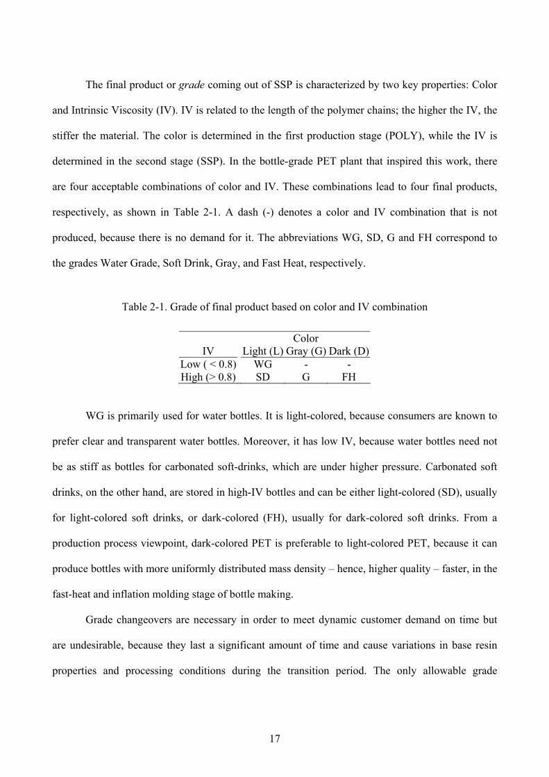
The final product or grade coming out of SSP is characterized by two key properties: Color

and Intrinsic Viscosity (IV). IV is related to the length of the polymer chains; the higher the IV, the

stiffer the material. The color is determined in the first production stage (POLY), while the IV is

determined in the second stage (SSP). In the bottle-grade PET plant that inspired this work, there

are four acceptable combinations of color and IV. These combinations lead to four final products,

respectively, as shown in Table 2-1. A dash (-) denotes a color and IV combination that is not

produced, because there is no demand for it. The abbreviations WG, SD, G and FH correspond to

the grades Water Grade, Soft Drink, Gray, and Fast Heat, respectively.

Table 2-1. Grade of final product based on color and IV combination

Color IV Light (L) Gray (G) Dark (D)

Low ( < 0.8) WG - - High (> 0.8) SD G FH

WG is primarily used for water bottles. It is light-colored, because consumers are known to

prefer clear and transparent water bottles. Moreover, it has low IV, because water bottles need not

be as stiff as bottles for carbonated soft-drinks, which are under higher pressure. Carbonated soft

drinks, on the other hand, are stored in high-IV bottles and can be either light-colored (SD), usually

for light-colored soft drinks, or dark-colored (FH), usually for dark-colored soft drinks. From a

production process viewpoint, dark-colored PET is preferable to light-colored PET, because it can

produce bottles with more uniformly distributed mass density – hence, higher quality – faster, in the

fast-heat and inflation molding stage of bottle making.

Grade changeovers are necessary in order to meet dynamic customer demand on time but

are undesirable, because they last a significant amount of time and cause variations in base resin

properties and processing conditions during the transition period. The only allowable grade

18

changeovers are from WG to SD to G to FH and backwards (always in this order). G is an

intermediate off-specification grade produced inevitably during the color changeover transition

from SD to FH and vice versa. Typically, there is no regular demand for it in the primary market for

PET, but it can be sold in a secondary market at a lower price. Another type of intermediate grade is

produced during the IV changeover transition from WG to SD and backwards. A common industrial

practice, which is also employed by the plant that inspired this work, is to divide this intermediate

grade into two halves and classify the first half as WG and the second half as SD. The opposite is

done in a changeover transition from SD to WG. Therefore, the entire quantity of the intermediate

grade is mixed in with the pure WG and SD grades and is sold in the primary market. In effect,

however, this mixing lowers the overall on-specification grade percentage, and is therefore highly

undesirable.

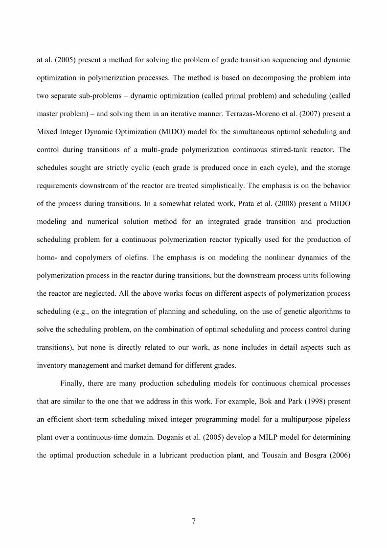
The two production stages, POLY and SSP, are separated by an intermediate storage area,

which we refer to as Temporary Storage Stage (TSS) and typically consists of 2-3 silos (see Figure

2-1). One possible way of using these silos would be to dedicate them to the different color grades

coming out of POLY. For example, if there were three TSS silos, then the first silo would be used

for storing Light-colored (L) PET, the second for storing gray (G) PET, and the third for storing

Dark-colored (D) PET. This way, if production were to change over, say, from light- to dark-

colored PET, the material coming out of POLY would have to be redirected from silo L to silo G,

during the color changeover transition period, and then to silo D upon the end of the transition.

Similarly, if the final grade production were to change over from SD to FH, then the silo feeding the

SSP reactor would have to be switched from L to D.

In effect, however, redirecting the feeds in and out of the TSS is not instantaneous but takes

a small transition time during which the grades before and after the changeover are mixed, because

the pipes in and out of the TSS must be emptied from one grade before they can be filled with the

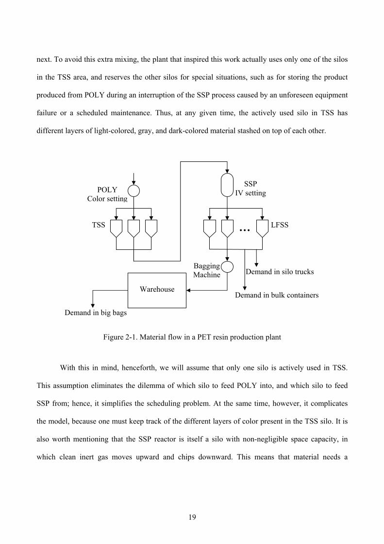
19

next. To avoid this extra mixing, the plant that inspired this work actually uses only one of the silos

in the TSS area, and reserves the other silos for special situations, such as for storing the product

produced from POLY during an interruption of the SSP process caused by an unforeseen equipment

failure or a scheduled maintenance. Thus, at any given time, the actively used silo in TSS has

different layers of light-colored, gray, and dark-colored material stashed on top of each other.

Figure 2-1. Material flow in a PET resin production plant

With this in mind, henceforth, we will assume that only one silo is actively used in TSS.

This assumption eliminates the dilemma of which silo to feed POLY into, and which silo to feed

SSP from; hence, it simplifies the scheduling problem. At the same time, however, it complicates

the model, because one must keep track of the different layers of color present in the TSS silo. It is

also worth mentioning that the SSP reactor is itself a silo with non-negligible space capacity, in

which clean inert gas moves upward and chips downward. This means that material needs a

…

Warehouse

POLY Color setting

SSP IV setting

TSS LFSS

BaggingMachine

Demand in bulk containers

Demand in silo trucks

Demand in big bags

20

significant time to travel through the reactor, and therefore what goes in SSP comes out from it with

a time delay. This adds another factor of complication to the model.

The grade coming out of SSP is loaded into one of several silos at the so-called Loading or

Final Storage Stage (LFSS). Unlike the silos in the TSS, which allow the cohabitation of different

colors, the silos in the LFSS do not. Thus, each silo can only contain a single final grade at any

given time. There is a degree of flexibility, however, in that it is possible to switch the grade that a

silo contains. In order for this to happen, though, the silo must first be completely emptied from one

grade, before it starts being filled with another.

The grade coming out of the silos in LFSS is either filled into big bags with the use of a

bagging machine and stored in a finished-goods warehouse, or is directly loaded into silo trucks or

bulk containers to be shipped to customers. A different unloading rate applies for each of these

three distinct unloading modes of the LFSS silos. Additionally, customers may also demand PET in

big bags directly from the warehouse. In this case, the big bags are loaded onto regular trucks.

The scheduling model that we develop in this chapter minimizes the cost associated with the

number of grade changeovers in a fixed time horizon, while also satisfying several constraints

related to sequence-dependent changeovers, sequential processing with production and space

capacity, mixed and flexible finite intermediate storage, and intermediate demand due-dates at both

the LFSS and the warehouse. We adopt a discrete-time representation, which keeps the model

relatively simple, enhances its flexibility and facilitates the introduction of additional constraints.

Furthermore, our computational results demonstrate that our model can handle practical problem

cases in quite reasonable times. Given the complexity of our model, which stems from the

complexity of the real system that it represents, we doubt that a continuous-time representation

would offer significant computational benefits.

21

The main input for the scheduling model is the initial setup state of POLY and SSP, the

initial inventory level and grade-type in TSS, LFSS and the warehouse, and the demand forecast for

each grade and transportation mode, in each period of the scheduling horizon. Given that the sales

department of the plant that motivated the development of our model can forecast the demand quite

accurately for a week ahead of time, a typical length of the scheduling horizon is one week. Within

this horizon, several scheduling decisions must be addressed, such as which grade to produce and

when to initiate a color or IV changeover transition, which LFSS silo to pour the grade coming out

of SSP into, which LFSS silo to sack big bags from, if any, and which LFSS silo to load trucks or

bulk containers from, to meet the demand.

The research presented in this chapter was conducted as part of a project entitled

“Optimization of production scheduling and product distribution of a PET resin chemical plant,” as

was mentioned in the acknowledgments section at the beginning of the dissertation. Having been

developed for a real Operations Research (OR) application, our model is tailor-made, because it

includes several features that are specific to this application and can not be incorporated into any of

the general-purpose, discrete-time or continuous-time model formulations that have been proposed

in the literature. These special features will become apparent in the following paragraphs, where we

describe in detail the operation of the PET plant that motivated this work. At the same time,

however, our model is general enough to be suitable for use in other similar applications,

particularly those in the polymer production industry, after performing the appropriate adjustments.

There are several features of our model which we have not encountered in the literature on

general-purpose MILP modeling in process scheduling. One such feature is that the changeover

sequence in one stage depends on the setup state of the other stage. More specifically, according to

Table 1, the changeover from low to high IV in SSP is not allowed, if the color setting of the

material currently being processed in SSP is G or D. This complicates things considerably, since the

22

color of the material being processed in SSP in a particular time period has been determined several

periods earlier when this material was processed in POLY. Moreover, as was also mentioned

earlier, even though the changeover transition time from low to high IV (and reversely) is

significant, in practice, the transition itself is conventionally considered to take place

instantaneously in the middle of the transition time, as far as the classification of the grade produced

by SSP is concerned. What complicates the model even more is that the SSP reactor has itself a

finite space capacity which introduces a delay between what goes in and out of SSP.

Another special feature of our model is that layers of different color grades are allowed to be

stored on top of each other in the active silo in TSS, making it necessary to keep track of these

layers. Consequently, the storage requirements of that silo do not fall in any of the usual types of

intermediate storage requirements encountered in the literature on MILP modeling in process

scheduling, namely, unlimited, finite dedicated or flexible (but with no mixing allowed), zero-wait,

and no storage requirements (e.g., see Shaik and Floudas (2007)). For this reason, we refer to these

requirements as mixed finite intermediate storage requirements.

Additionally, the demand for final products does not only occur at different intermediate

dates, but also at two different storage stages, namely, at the LFSS and at the warehouse. This

makes the LFSS both an intermediate and a final storage area, raising the question “to sack or not to

sack big bags,” because sacking big bags serves to increase the service level of customers

requesting big bags from the warehouse but at the same time lowers the service level of customers

requesting bulk material from the silos at the LFSS.

The above features complicate the mathematical formulation of our model but also make it

more interesting and challenging. The real motivation for developing our model, however, stems

from the fact that it is built for a real OR application. We present a case study that illustrates the

application of the model on a real problem scenario and provides insight into its behavior. The

23

numerical experience that we provide demonstrates that the computational requirements of the

model are quite reasonable for problem sizes that typically arise in practical applications.

2.2 MILP model development

For the needs of our model, we discretize time by dividing the scheduling horizon, typically one

week, into a finite number of identical time periods. The length of each period must be no bigger

than the length of the shortest nonstop event that takes place in the entire process. This could be the

transition time of a grade changeover, the time of a shift, if different shifts have different

characteristics, etc.

The production facility operates on a 24-hour basis, so in each period, POLY produces an

amount of material which is equal to the constant production rate of the plant, denoted by P,

multiplied by the length of the period; therefore, POLY is considered as a source of material (we

assume that it is never starved of raw material), and the material that it produces in each period is

referred to as a lot.

The next step is to discretize space at the TSS and SSP stages by dividing their capacities

into an integer number of slots, where each slot accommodates exactly one lot. At the beginning of

the scheduling horizon, the active silo in the TSS has some initial material in it that occupies several

slots – say N slots – and the SSP reactor is filled with material up to its capacity, which is equal to,

say, M slots. The SSP reactor has the same production rate as POLY, as was mentioned in Section

2.1; therefore, in each period, the TSS and the SSP stages consume from their upstream stage and

release into their downstream stage exactly one lot. This implies that in every period of the

scheduling horizon, the number of lots in TSS and SSP is constant and equal to N and M,

respectively.

24

Note that if the production rates of POLY and SSP were allowed to be different, then we

would have to keep track of the dynamically changing level of material (number of non-empty

slots) in the TSS, as well as the type of material in each slot. In fact, this is more or less what we do

in the case of the LFSS, where the input rate is constant but the output rate is partly variable and

uncontrollable, due to the varying demand, and partly controllable, as the rate of bagging bulk

material from the LFSS into big bags is a decision variable.

The color (L, G or D) of the lot in the nth slot of the N + M slots of the TSS and the SSP

reactor taken together depends on the setup state (L, G or D) of POLY n periods before the

beginning of the time horizon. Therefore, in order to characterize the color in the N + M slots of the

TSS and the SSP reactor, we need to know the setup state of POLY during the last N + M periods

before the beginning of the scheduling horizon. With this in mind, we shift the time axis by N + M

periods so that the first period of the scheduling horizon is N + M + 1, and therefore periods 1 to N

+ M refer to the past.

Next, we present the MILP formulation that we developed for the problem under

consideration. The following notation is used:

Sets:

I : set of colors produced by POLY, indexed by i, I = 1, 2, 3 ≡ L, G, D

J : set of final grades, indexed by j, J = 1, 2, 3, 4 ≡ WG, SD, G, FH

Q : set of silos in LFSS, indexed by q

Parameters:

T : index of the last period of the scheduling horizon

P : production quantity of the process in one period

N : number of slots in TSS

M : number of slots in SSP

25

d : cost incurred per color changeover at POLY

c : cost incurred per IV changeover at SSP

B : duration of a color changeover transition at POLY (in number of periods)

F : duration of an IV changeover transition at SSP (in number of periods)

X01t : binary parameter that takes the value 1 if the lot produced by POLY in period t has color L,

and 0 otherwise, t = 1,…, N + M

X02t : binary parameter that takes the value 1 if the lot produced by POLY in period t has color G,

and 0 otherwise, t = 1,…, N + M

X03t : binary parameter that takes the value 1 if the lot produced by POLY in period t has color D,

and 0 otherwise, t = 1,…, N + M

A0t : binary parameter that takes the value 1 if an IV change is initiated at the beginning of period

t, and 0 otherwise, t = N + M – F + 2,…, N + M

Z0: binary parameter that takes the value 1 if the IV of the lot stored in the last slot of SSP at the

beginning of the scheduling horizon is high, and 0 otherwise

W0qj : binary parameter that takes the value 1 if grade j is stored in silo q of LFSS at the beginning

of the scheduling horizon, and 0 otherwise

S0qj : quantity of grade j contained in silo q of LFSS at the beginning of the scheduling horizon

Smax : capacity of a silo in LFSS

Smin : minimum quantity of a nonempty silo in LFSS

SSmin j : safety stock of grade j in LFSS at the end of the scheduling horizon

uST : maximum quantity of material that can be loaded from LFSS into a silo truck in one period

uBC : maximum quantity of material that can be loaded from LFSS into a bulk container in one

period

uBΒ : maximum quantity of material that can be sacked from LFSS into big bags in one period

26

R0j : grade j inventory in the warehouse at the beginning of the scheduling horizon

Rmax : warehouse capacity

Rmin j : safety stock of grade j in the warehouse at the end of the scheduling horizon

dSTjt: silo trucks demand of grade j in period t, t = N + M + 1,…, T

dBCjt: bulk containers demand of grade j in period t, t = N + M + 1,…, T

dBBjt: big bags demand of grade j in period t, t = N + M + 1,…, T

Decision Variables:

xit : binary decision variable that takes the value 1 if the lot produced by POLY in period t has

color i, and 0 otherwise, t = 1,…, T

yjt : binary decision variable that takes the value 1 if final grade j is produced by SSP in time

period t, and 0 otherwise, t = N + M + 1,…, T + (F/2)

at : binary decision variable that takes the value 1 if an IV changeover is initiated at the

beginning of period t, and 0 otherwise, t = N + M – F + 2,…, T

zt : binary decision variable that takes the value 1 if the IV of the grade produced in period t is

high, and 0 otherwise, t = N + M,…, T + (F/2)

Sqjt : quantity of grade j in silo q of LFSS at the end of period t, t = N + M,…, T

Wqjt : binary decision variable that takes the value 1 if grade j is contained in silo q of LFSS in

period t, and 0 otherwise, t = N + M,…, T

gqjt : binary decision variable that takes the value 1 if grade j is loaded from SSP into silo q of

LFSS in period t, and 0 otherwise, t = N + M + 1,…, T

Gqjt : quantity of grade j that is unloaded from silo q of LFSS in period t, t = N + M + 1,…, T

bqjt: quantity of grade j that is loaded from silo q of LFSS into big bags in period t, t = N + M +

1,…, T

fqjt : quantity of grade j that is loaded from silo q of LFSS into silo trucks in period t, t = N + M +

27

1,…, T

hqjt : quantity of grade j that is loaded from silo q of LFSS into bulk containers in period t, t = N +

M + 1,…, T

Rjt : quantity of grade j in the warehouse at the end of period t, t = N + M,…, T

The formulation that we develop next also assumes that the following inequalities hold: F <

N + M, B < N + M, N + M < T – (N + M). These restrictions hold in practice.

The objective function of our model is expressed as

21 1

1Minimize T T

t tt N M t N M

c a d xB= + + = + +

⎛ ⎞ ⎛ ⎞+⎜ ⎟ ⎜ ⎟⎝ ⎠ ⎝ ⎠∑ ∑ (2.1)

The above expression minimizes the weighted sum of the number of IV and color

changeovers during the scheduling horizon, i.e., from period N + M + 1 to period T. The first

summation in the objective function represents the number of IV changeovers. The second

summation represents the total number of color changeover transition periods. It is divided by B,

i.e., by the duration of a color changeover transition, to give the number of color changeovers.

Next, we present the constraints of our model. Constraints (2.2)-(2.11) are related to the

processing part of the plant, which comprises POLY, TSS and SSP.

1iti I

x∈

=∑ , t = 1, …, T (2.2)

1 3

3 1

1

1t t p

t t p

x x

x x+

+

+ ≤ ⎫⎪⎬+ ≤ ⎪⎭

, t = 1,…, T – 1, p = 1, …, min(T – t, B) (2.3)

1 3 1

3 1 1

11

t t

t t

y yy y

+

+

+ ≤ ⎫⎬+ ≤ ⎭

, t = N + M + 1,…, T + (F/2) – 1 (2.4)

Constraint set (2.2) states that POLY can only produce a single color in each period. Since

the color of the final grade exiting SSP in any period was determined in POLY N + M periods

earlier, at the beginning of the scheduling horizon, the color in slots 1,…, N + M has already been

28

predetermined; therefore, in effect, constraint (2.2) must really be imposed from period N + M + 1

and on only. Its application to periods 1,…, N + M is merely a routine check that serves to verify

that the initial status of the system, as decided in the previous scheduling horizon, results in feasible

production settings during the present horizon, too. This modeling technique is also adopted in

several of the other model constraints which follow.

Constraint set (2.3) states that between two periods in which POLY produces colors L and D

(in either order), B periods in which POLY produces G must always intervene. Note that the actual

number of constraints of this set depends not only on the length of the scheduling horizon but also

on the value of B. More specifically, if B = 1, then POLY can not produce colors D and L in two

adjacent periods. If B > 1, this restriction is imposed not only to adjacent periods, but also to periods

that are spaced i periods apart, for i = 2,…, B.

Similarly, constraint set (2.4) states that final grades WG and G can not be produced in two

adjacent periods, because at least one period in which grade SD is produced must always intervene.

Since the color is determined in POLY and any IV change in SSP becomes effective F/2 periods

after it is initiated, the final grade that will be produced in the first F/2 periods of the scheduling

horizon, i.e., in periods N + M + 1,…, N + M + (F/2), is predetermined by the initial state of the

system. Therefore, constraint set (4) must really be imposed from period N + M + (F/2) and on only.

Its application to periods N + M,…, N + M + (F/2) – 1 serves to verify that the initial conditions are

feasible. To ensure that the current production schedule will also remain feasible in the next

scheduling horizon, this set of constraints also extends to periods T + 1,…, T + (F/2) – 1. Combined

together, constraint sets (2.3) and (2.4) ensure that the only allowable grade changeovers are from

WG to SD to G to FH and backwards, always in this exact sequence.

1

1t F

ss t

a+ −

=

≤∑ , t = N + M – F + 2, …, T – F + 1 (2.5)

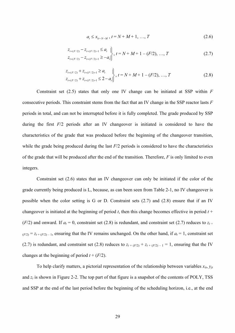
29

1t t N Ma x − −≤ , t = N + M + 1, …, T (2.6)

( / 2) ( / 2) 1

( / 2) ( / 2) 1

t F t F t

t F t F t

z z a

z z a+ + −

+ + −

− ≤ ⎫⎪⎬− ≥ − ⎪⎭

, t = N + M + 1 – (F/2), …, T (2.7)

( / 2) ( / 2) 1

( / 2) ( / 2) 1 2t F t F t

t F t F t

z z a

z z a+ + −

+ + −

+ ≥ ⎫⎪⎬+ ≤ − ⎪⎭

, t = N + M + 1 – (F/2), …, T (2.8)

Constraint set (2.5) states that only one IV change can be initiated at SSP within F

consecutive periods. This constraint stems from the fact that an IV change in the SSP reactor lasts F

periods in total, and can not be interrupted before it is fully completed. The grade produced by SSP

during the first F/2 periods after an IV changeover is initiated is considered to have the

characteristics of the grade that was produced before the beginning of the changeover transition,

while the grade being produced during the last F/2 periods is considered to have the characteristics

of the grade that will be produced after the end of the transition. Therefore, F is only limited to even

integers.

Constraint set (2.6) states that an IV changeover can only be initiated if the color of the

grade currently being produced is L, because, as can been seen from Table 2-1, no IV changeover is

possible when the color setting is G or D. Constraint sets (2.7) and (2.8) ensure that if an IV

changeover is initiated at the beginning of period t, then this change becomes effective in period t +

(F/2) and onward. If at = 0, constraint set (2.8) is redundant, and constraint set (2.7) reduces to zt +

(F/2) = zt + (F/2) – 1, ensuring that the IV remains unchanged. On the other hand, if at = 1, constraint set

(2.7) is redundant, and constraint set (2.8) reduces to zt + (F/2) + zt + (F/2) – 1 = 1, ensuring that the IV

changes at the beginning of period t + (F/2).

To help clarify matters, a pictorial representation of the relationship between variables xit, yjt

and zt is shown in Figure 2-2. The top part of that figure is a snapshot of the contents of POLY, TSS

and SSP at the end of the last period before the beginning of the scheduling horizon, i.e., at the end

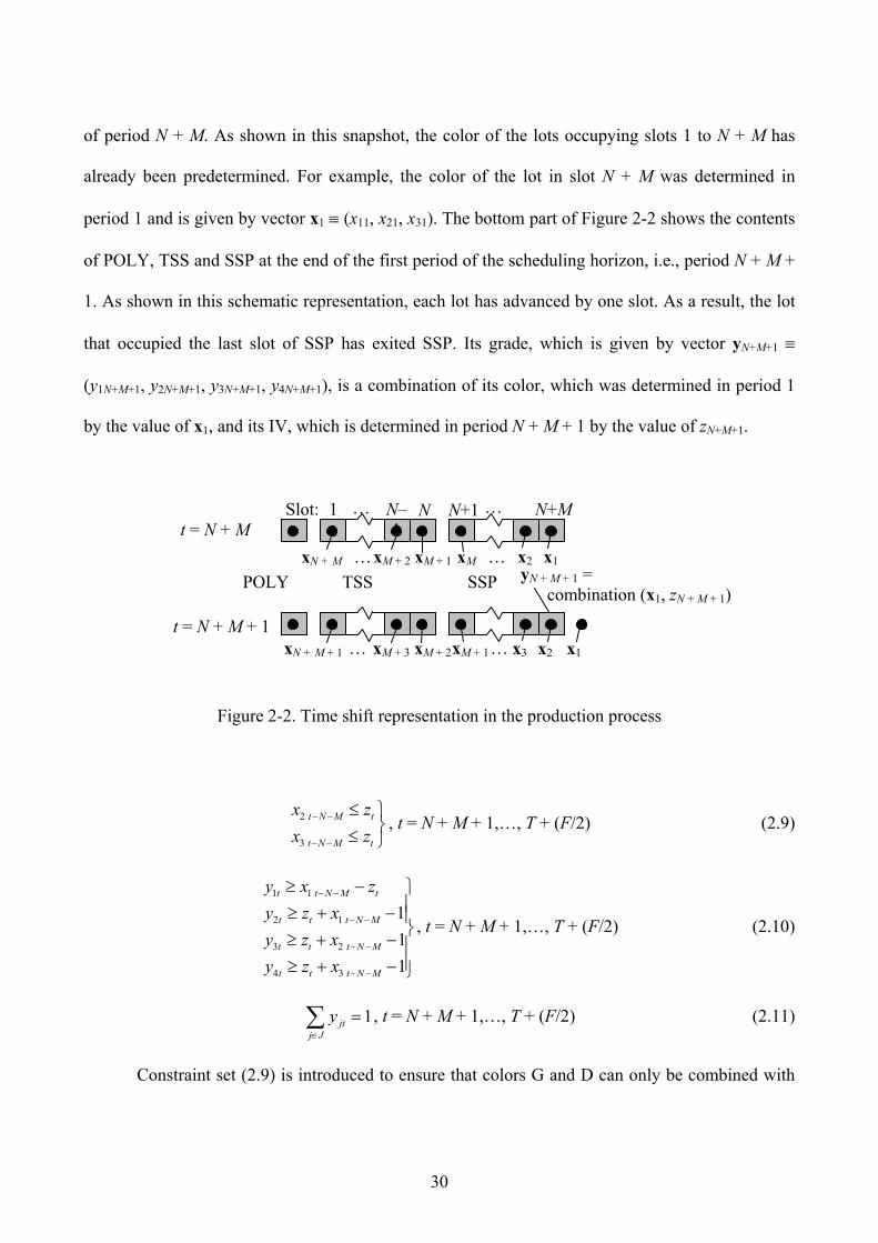
30

of period N + M. As shown in this snapshot, the color of the lots occupying slots 1 to N + M has

already been predetermined. For example, the color of the lot in slot N + M was determined in

period 1 and is given by vector x1 ≡ (x11, x21, x31). The bottom part of Figure 2-2 shows the contents

of POLY, TSS and SSP at the end of the first period of the scheduling horizon, i.e., period N + M +

1. As shown in this schematic representation, each lot has advanced by one slot. As a result, the lot

that occupied the last slot of SSP has exited SSP. Its grade, which is given by vector yN+M+1 ≡

(y1N+M+1, y2N+M+1, y3N+M+1, y4N+M+1), is a combination of its color, which was determined in period 1

by the value of x1, and its IV, which is determined in period N + M + 1 by the value of zN+M+1.

Figure 2-2. Time shift representation in the production process

2

3

t N M t

t N M t

x zx z

− −

− −

≤ ⎫⎬≤ ⎭

, t = N + M + 1,…, T + (F/2) (2.9)

1 1

2 1

3 2

4 3

111

t t N M t

t t t N M

t t t N M

t t t N M

y x zy z xy z xy z x

− −

− −

− −

− −

≥ − ⎫⎪≥ + − ⎪⎬≥ + − ⎪⎪≥ + − ⎭

, t = N + M + 1,…, T + (F/2) (2.10)

1jtj J

y∈

=∑ , t = N + M + 1,…, T + (F/2) (2.11)

Constraint set (2.9) is introduced to ensure that colors G and D can only be combined with

yN + M + 1 = combination (x1, zN + M + 1)

POLY TSS SSP

xM + 2xM + 1xM + 3 ……xN + M + 1 x3 x2 x1

xN + M xM + 2 xM + 1 xM x1x2… …t = N + M

t = N + M + 1

1 N–1

N N+1 N+MSlot: … …

31

high IV. Constraint set (2.10) determines the final grade based on the combination of color and IV,

while constraints (2.11) state that only a single grade can be produced in any period of the

scheduling horizon. If status verification is not necessary, constraints (2.9)-(2.11) can be applied

from period N + M + (F/2) + 1 and on.

Constraint sets (2.12)-(2.29) are related to the storage part of the plant, which comprises

LFSS and the warehouse.

qjt qjtg W≤ , q ∈ Q, j ∈ J, t = N + M + 1,…, T (2.12)

qjt jtq

g y≤∑ , j ∈ J, t = N + M + 1,…, T (2.13)

1qjtq Q j J

g∈ ∈

=∑∑ , t = N + M + 1,…, T (2.14)

1qjtj J

W∈

≤∑ , q ∈ Q, t = N + M + 1,…, T (2.15)

∑∈

+ −≤−Jr

qrtqjtqjt WWW 11 , q ∈ Q, j ∈ J, t = N + M,…, T – 1 (2.16)

Constraint set (2.12) ensures that in each period, grade j can not be loaded from SSP into

silo q of the LFSS, unless this silo already has grade j in it at the beginning of this period.

Constraint (2.13) ensures that in each period, the grade loaded into any silo of the LFSS is the same

with the grade that is being produced by SSP in the same period. Constraint set (2.14) ensures that

in each period, a single grade will be loaded from SSP into a single silo of LFSS. Constraint set

(2.15) states that in each period, each silo of the LFSS can store at most one grade.

Constraint set (2.16) states that the grade stored in a silo of the LFSS can not change unless

a period in which this silo is empty intervenes. The summation qrtr JW

∈∑ is equal to 1 when silo q

contains some final grade in period t, and 0 if it is empty. Thus, a difference equal to 0 in the right-

hand side forces the difference in the left-hand side to be 0, ensuring that any grade j which is

different from the one that was contained in the silo in the previous period, can not be poured in this

32

silo before it is completely emptied. Note that index j is used in both terms of the left-hand side to

disclose whether a particular grade j can be poured into silo q in period t + 1, while r is used in the

right-hand side to disclose whether silo q contained any final grade r in the previous period.

maxqjt qjtS S W≤ , q ∈ Q, j ∈ J, t = N + M + 1,…, T (2.17)

minqjt qjtS S W≥ , q ∈ Q, j ∈ J, t = N + M + 1,…, T (2.18)

max( , , )qjt qjt ST BC BBG W u u u≤ , q ∈ Q, j ∈ J, t = N + M + 1,…, T (2.19)

1qjt qjt qjt qjtS S g P G−= + − , q ∈ Q, j ∈ J, t = N + M + 1,…, T (2.20)

∑∈

≥Qq

jnmqjT SSS i , j ∈ J (2.21)

Constraint set (2.17) states that the grade quantity stored in a silo can not exceed the silo’s

capacity, and ensures that it will be zero whenever the corresponding variable W determines that

this silo is empty. Constraint set (2.18) imposes a lower bound on the quantity of a nonempty silo. It

is introduced to eliminate the situation in which a silo stores a negligible but positive grade

quantity. Constraint set (2.19) states that no grade can be unloaded from an empty silo and imposes

the maximum rate in which a silo can be unloaded, based on the values of variables u. Constraint set

(2.20) ensures flow continuity, by updating the quantity stored in each silo, based on the quantity

that it contained in the previous period, and the quantities loaded into and out of it in the next

period. Note that the quantity produced by POLY and SSP in one period and all the quantities that

can be unloaded or sacked from the LFSS depend on the period length. Constraint set (2.21) ensures

that the total inventory of each grade in the LFSS is at or above the specified safety stock for that

grade at the end of the scheduling horizon.

qjt qjt qjt qjtG f h b= + + , q ∈ Q, j ∈ J, t = N + M + 1,…, T (2.22)

11 1 1

qjt qjt qjtST BC BB

bf hu u u

+ + ≤ , q ∈ Q, j ∈ J, t = N + M + 1,…, T (2.23)

33

jt qjtq Q

dST f∈

= ∑ , j ∈ J, t = N + M + 1,…, T (2.24)

jt qjtq Q

dBC h∈

= ∑ , j ∈ J, t = N + M + 1,…, T (2.25)

∑∑∈ ∈

≤Qq

BBJj

qjt ub , t = N + M + 1,…, T (2.26)

1jt jt qjt jtq Q

R R b dBB−∈

= + −∑ , j ∈ J, t = N + M + 1,…, T (2.27)

maxjtj J

R R∈

≤∑ , t = N + M + 1,…, T (2.28)

jnmjT RR i≥ , j ∈ J (2.29)

Constraint set (2.22) states that, in each period, the total quantity of grade j unloaded from

any silo of the LFSS is equal to the quantity that is loaded into silo trucks or bulk containers, or

sacked into big bags and stored in the warehouse. Constraint set (2.23) defines the maximum

unloading rate of any silo, based on the exact unloading mode. Constraint sets (2.24) and (2.25)

ensure that the demand for silo trucks and bulk containers is satisfied for each period of the

scheduling horizon. Constraint set (2.26) ensures that the maximum sacking rate is not exceeded.

Note that, while several silos can be used simultaneously for loading silo trucks or bulk containers,

bagging can only take place in one silo, because only one bagging machine is available. Constraint

set (2.27) updates the inventory stored in the warehouse, and constraint set (2.28) ensures that the

total grade quantity stored in the warehouse does not exceed its capacity. Finally, constraint set

(2.29) ensures that the inventory of each grade in the warehouse is at or above the specified safety

stock at the end of the scheduling horizon.

Constraints (2.30)-(2.35) initialize the state of the system at the beginning of the scheduling

horizon.

itit Xx 0= , i ∈ I, t = 1,…, N + M (2.30)

34

0Zz MN =+ (2.31)

tt Aa 0= , t = N + M – F + 2,…, N + M (2.32)

qjqjt SS 0= , q ∈ Q, j ∈ J, t = N + M (2.33)

qjqjt WW 0= , q ∈ Q, j ∈ J, t = N + M (2.34)

jjt RR 0= , j ∈ J, t = N + M (2.35)

More specifically, constraint sets (2.30)-(2.32) initialize the state of the production system at

the beginning of the scheduling horizon. Note that, at the beginning of the scheduling horizon, the

color has already been predetermined for all the in-process lots in TSS and SSP. Therefore, one

needs to initialize the values of variables xit, i∈I, for t = 1 to N + M. Also, the initialization of

variables at for the last F – 1 periods is required, since at most one IV change can be initiated within

F consecutive periods. Note, however, that at the beginning of the scheduling horizon, the IV has

already been predetermined for the last F/2 slots of the SSP reactor only, since it takes F/2 periods

for an IV changeover to take place. Yet, only the value of variable zt, for t = N + M needs to be

initialized, since the remaining (F/2) – 1 values are determined through constraint sets (2.7)-(2.8)

and variables at. As a consequence, the final grade that will be produced in the first F/2 periods of

the scheduling horizon is already predetermined, too. Constraint sets (2.33)-(2.35) initialize the

inventories in the LFSS silos and the warehouse at the beginning of the scheduling horizon.

xit binary; i ∈ I, t = 1,…, T (2.36)

yjt binary; j ∈ J, t = N + M + 1,…, T + (F/2) (2.37)

at binary; t = N + M-F + 2,…, T (2.38)

zt binary; t = N + M,…, T + (F/2) (2.39)

wqit binary; q ∈ Q, j ∈ J, t = N + M,…, T (2.40)

gqit binary; q ∈ Q, j ∈ J, t = N + M + 1,…, T (2.41)

35

0qjtG ≥ , q ∈ Q, j ∈ J, t = N + M + 1,…, T (2.42)

0jtR ≥ , j ∈ J, t = N + M, …, T (2.43)

0qjtS ≥ , q ∈ Q, j ∈ J, t = N + M,…, T (2.44)

0qjtb ≥ , q ∈ Q, j ∈ J, t = N + M + 1,…, T (2.45)

0qjtf ≥ , q ∈ Q, j ∈ J, t = N + M + 1,…, T (2.46)

0qjth ≥ , q ∈ Q, j ∈ J, t = N + M + 1,…, T (2.47)

Finally, constraint sets (2.36)-(2.41) and (2.42)-(2.47) impose the integrality and the

nonnegativity of the decision variables, respectively. Note that the indexing of variables yjt begins

from t = N + M + 1 instead of t = N + M + (F/2) + 1, in order to keep record of the final grade

produced during the first F/2 periods, too, which was actually determined by the production

schedule of the previous horizon.

Note that in the above formulation we have assumed that at the beginning of the scheduling

horizon, the plant is in the state that it was left off at the end of the previous horizon, because this is

the usual situation encountered in practice. There also exists the situation where the plant is just

beginning its operations after a long shutdown, in which case, all the slots of TSS and SSP are

empty and possibly the silos and the warehouse are at very low or even zero levels. This situation is

very rare in practice and is typically encountered after a major breakdown or after the yearly

maintenance of the plant. When the plant is starting up after a long shutdown, the main concern is to

stabilize the process and get the production going, rather than solving the scheduling problem. In

principle, however, our model can still address the scheduling problem during the startup (or warm

up) period, by letting period 1 (instead of period N + M + 1) be the first period of the scheduling

horizon and appropriately adjusting the sets of time indices for which the constraints hold.

36

Also note that constraint sets (2.24), (2.25) and (2.27) ensure that the demand for silo trucks,

bulk containers and big bags is satisfied for each period of the scheduling horizon. The strict

requirement for on-time satisfaction of the demand stems from the current practice of the plant that

motivated this work. Specifically, the customers of the plant schedule to send their own (or third

party) trucks or containers to pick up their orders on specific periods, and can not afford to wait.

This requirement may seem restrictive, because it may lead to infeasibilities, but in practice, it does

not pose a problem, because the capacities of the LFSS and the warehouse are big enough to absorb

any reasonable variations in the demand. Moreover, the careful choice of safety stock levels for

each grade and inventory stage (LFSS and warehouse) can help minimize the number of

changeovers in the long run, while preventing stockouts and production process blocking due to the

lack of storage space. In the following section, we present an application in which we set the

scheduling horizon equal to one week that is discretized into 42 4-hour periods, and solved our

model sequentially 24 times (weeks), i.e., for a total of 6 months, where at the beginning of each

week, the state of the system was set equal to the state that it ended up in the previous week. We

used real demand data for each week, and we did not encounter any infeasibility problems. The

safety stock levels were carefully chosen by modeling and solving the continuous-process

scheduling problem as a Stochastic Economic Lot Scheduling Problem (SELSP), as described in

Chapter 3.

Still, in applications where the on-time satisfaction of demand is not a strict requirement, we

can easily modify our model, by including in the objective function the following penalty cost term

for not satisfying the demand on time:

( )1 3 1

T t

j qj j qj j jt N M j J N M q Q q Q

e dST f dBC h dBB dbτ τ τ τ τ ττ= + + ∈ − = + + ∈ ∈

⎛ ⎞⎡ ⎤⎛ ⎞ ⎛ ⎞− + − + −⎜ ⎟⎢ ⎥⎜ ⎟ ⎜ ⎟⎜ ⎟⎢ ⎥⎝ ⎠ ⎝ ⎠⎣ ⎦⎝ ⎠

∑ ∑ ∑ ∑ ∑ ,

37

where e denotes the stockout penalty cost coefficient, and dbjt denotes the quantity of product j that

is used to satisfy the demand for big bags in period t. In this case, constraints (2.24), (2.25) and

(2.27) need to be modified, as follows:

1 1

t t

j qjN M N M q Q

dST fτ ττ τ= + + = + + ∈

≥∑ ∑ ∑ , j ∈ J, t = N + M + 1,…, T

1 1

t t

j qjN M N M q Q

dBC hτ ττ τ= + + = + + ∈

≥∑ ∑ ∑ , j ∈ J, t = N + M + 1,…, T

1jt jt qjt jtq Q

R R b db−∈

= + −∑ , j ∈ J, t = N + M + 1,…, T

and the following constraint must be added to the model:

1 1

t t

j qjN M N M q Q

dBB dbτ ττ τ= + + = + + ∈

≥∑ ∑ ∑ , j ∈ J, t = N + M + 1,…, T.

Finally, we may further modify our model in a similar manner, by replacing the hard

constraints (2.21) and (2.29), which require that the inventory levels at the end of the horizon be no

less than the safety stock levels, with an extra term in the objective function, that penalizes any

negative deviations of the inventory levels at the end of the horizon from the safety stock levels.

2.3 Application of the model

In this section, we illustrate the application of the MILP model that we developed in the previous

section on a problem instance drawn from the operation of the plant that inspired this work. The

production rate of the facility is 200 tons/day, which is what the plant uses most of the time,

although in the long run it can vary between 180 and 220 tons/day. The color changeover transition

time between L and D in POLY is 4 hours, while the IV changeover transition between low and

high IV in SSP is 24 hours. Both transition times are divisible by 4; hence, for the purposes of time

discretization, we use a 4-hour time period. This makes B = 1, F = 6, and the production rate equal

38

to 33.3 tons/period. Note that a 4-hour period is also convenient because it is a divisor of a 24-hour

day and of a typical 8-hour work-shift.

The active silo at the TSS has a capacity of 430 tons but is usually less than half full. With

this in mind, we assume that at the beginning of the scheduling horizon it has 200 tons of material

in it. This initial quantity can be divided into N = 6 identical slots, each with a capacity of 33.33

tons (the amount produced in a period). Similarly, the SSP reactor, which has a capacity of 200

tons, can be divided into M = 6 identical slots, each with a capacity of 33.33 tons.

In the actual operation of the plant, production is scheduled on a weekly basis, because at

the end of each week, the demand during the following week is known with certainty. With this in

mind, we use a scheduling horizon of one week, i.e., 42 time periods. Given that N = M = 6, the first

period of the scheduling horizon is period 13 (= N + M + 1), and the last period, T, is period 54 (= N

+ M + 42). The values of the other problem parameters are Z0 = 1, Smax = 430 tons, Smin = 1 ton,

Rmax = 3500 tons, uST = 224 tons, uBC = 69.2 tons, uBB = 40 tons, c = 1, d = 1.

We solved the MILP model sequentially, for 24 weeks, i.e., 6 months, using real demand

data. For space consideration, the demand values for each period are shown in Appendix A. In

Table 2-2, we show the sample mean and standard deviation of the daily demand, for each grade

and demand type. Note that the total mean daily demand for all grades and types is ~195 tons,

which is slightly below the production rate of 200 tons per day. This small difference between

production capacity and demand is due to the unavoidable production of grade 3 (G), which takes

away some of the production capacity. As was mentioned earlier, there is no scheduled demand for

grade G; in reality, however, the plant occasionally removes the accumulated inventory of grade G

by selling it at a lower price to interested buyers. Also, note that grade 2 (SD) is only demanded in

big bags.

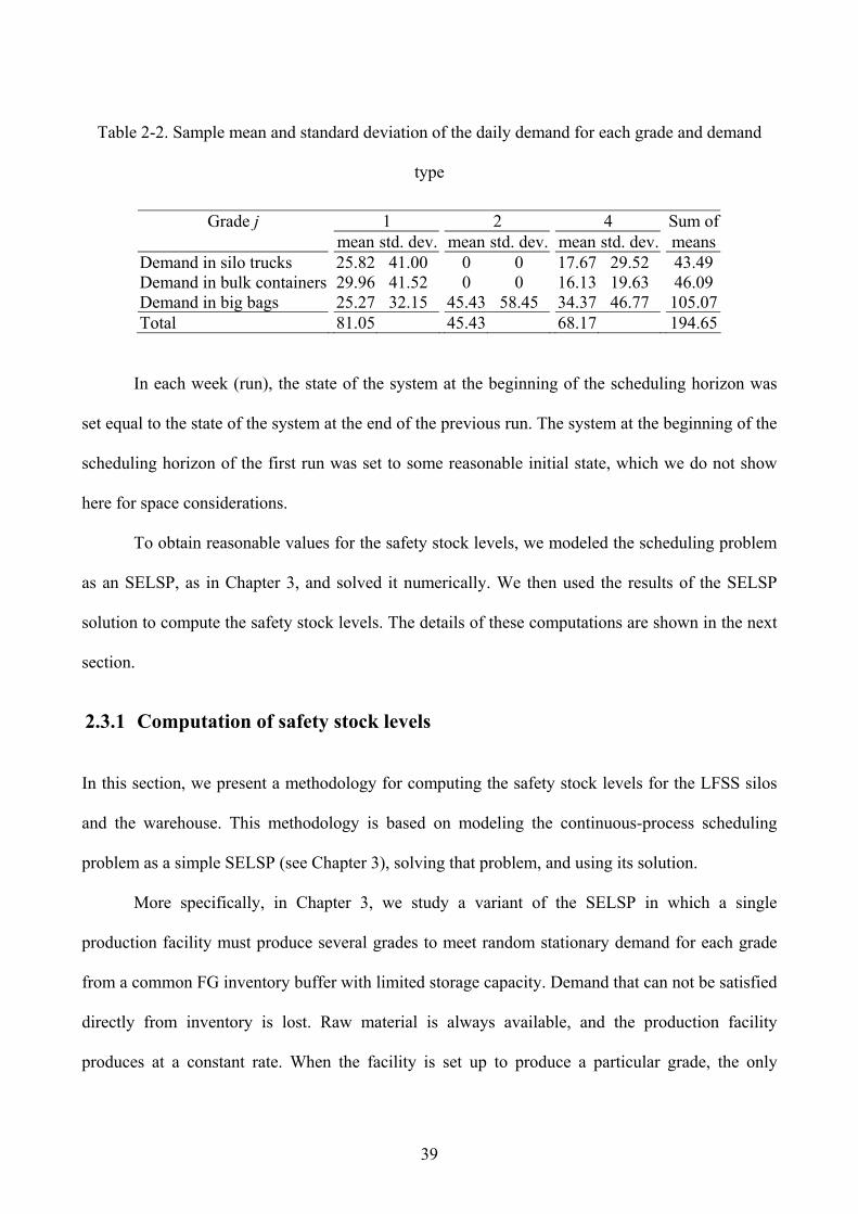
39

Table 2-2. Sample mean and standard deviation of the daily demand for each grade and demand

type

Grade j 1 2 4 Sum of mean std. dev. mean std. dev. mean std. dev. meansDemand in silo trucks 25.82 41.00 0 0 17.67 29.52 43.49Demand in bulk containers 29.96 41.52 0 0 16.13 19.63 46.09Demand in big bags 25.27 32.15 45.43 58.45 34.37 46.77 105.07Total 81.05 45.43 68.17 194.65

In each week (run), the state of the system at the beginning of the scheduling horizon was

set equal to the state of the system at the end of the previous run. The system at the beginning of the

scheduling horizon of the first run was set to some reasonable initial state, which we do not show

here for space considerations.

To obtain reasonable values for the safety stock levels, we modeled the scheduling problem

as an SELSP, as in Chapter 3, and solved it numerically. We then used the results of the SELSP

solution to compute the safety stock levels. The details of these computations are shown in the next

section.

2.3.1 Computation of safety stock levels

In this section, we present a methodology for computing the safety stock levels for the LFSS silos

and the warehouse. This methodology is based on modeling the continuous-process scheduling

problem as a simple SELSP (see Chapter 3), solving that problem, and using its solution.

More specifically, in Chapter 3, we study a variant of the SELSP in which a single

production facility must produce several grades to meet random stationary demand for each grade

from a common FG inventory buffer with limited storage capacity. Demand that can not be satisfied

directly from inventory is lost. Raw material is always available, and the production facility

produces at a constant rate. When the facility is set up to produce a particular grade, the only

40

allowable changeovers are from that grade to the next lower or higher grade. All changeover times

are deterministic and equal to each other. There is a changeover cost per changeover occasion, a

spill-over cost per unit of product in excess, whenever there is not enough space in the FG buffer to

store the produced grade, and a lost-sales cost per unit short, whenever there is not enough FG

inventory to satisfy demand. We model the SELSP as a discrete-time Markov Decision Process

(MDP), where in each time period it must be decided whether to initiate a changeover to a

neighboring grade or keep the setup of the production facility unchanged, based on the current state

of the system, which is determined by the current setup of the facility and the FG inventory levels

of all the grades. The goal is to minimize the infinite-horizon expected average cost. For 2-grade

and 3-grade problems we numerically solve the resulting MDP problem using successive

approximations. The solution includes the optimal state-dependent policy and the optimal

differential cost (value function) for each state of the system. The optimal policy partitions the state

space into different regions, each characterized by a different optimal changeover action. The FG

inventory levels at which the value function is minimized for a given setup state are the “ideal”

target inventory levels for that setup state and in that sense can be thought of as the optimal safety

stock levels for that state. In other words, the optimal safety stock levels really depend on the setup

state of the facility.

We used the above methodology to find the optimal safety stock levels for a 3-grade system,

where the three grades are WG, SD, and FH. To this end, we discretized the inventory space and

time, and we used a demand distribution for each grade based on the real demand data for 6 months

that we had available, without differentiating between the individual types of demand (silo trucks,

bulk containers and big bags). The optimal safety stock level of grade j, when the facility is set up

to produce grade i, denoted by Imin,i,j, is shown in Table 2-3. Note that the safety stock levels

strongly depend on the setup of the facility. For example, the safety stock level for WG is only 60

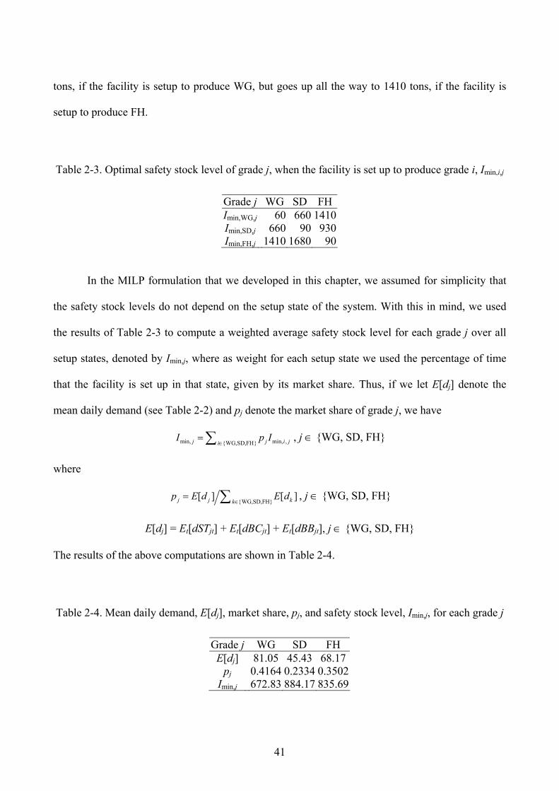
41

tons, if the facility is setup to produce WG, but goes up all the way to 1410 tons, if the facility is

setup to produce FH.

Table 2-3. Optimal safety stock level of grade j, when the facility is set up to produce grade i, Imin,i,j

Grade j WG SD FHImin,WG,j 60 660 1410Imin,SD,j 660 90 930Imin,FH,j 1410 1680 90

In the MILP formulation that we developed in this chapter, we assumed for simplicity that

the safety stock levels do not depend on the setup state of the system. With this in mind, we used

the results of Table 2-3 to compute a weighted average safety stock level for each grade j over all

setup states, denoted by Imin,j, where as weight for each setup state we used the percentage of time

that the facility is set up in that state, given by its market share. Thus, if we let E[dj] denote the

mean daily demand (see Table 2-2) and pj denote the market share of grade j, we have

min, min, ,WG,SD,FHj j i jiI p I

∈=∑ , j ∈ WG, SD, FH

where

WG,SD,FH

[ ] [ ]j j kkp E d E d

∈= ∑ , j ∈ WG, SD, FH

E[dj] = Et[dSTjt] + Et[dBCjt] + Et[dBBjt], j ∈ WG, SD, FH

The results of the above computations are shown in Table 2-4.

Table 2-4. Mean daily demand, E[dj], market share, pj, and safety stock level, Imin,j, for each grade j

Grade j WG SD FH E[dj] 81.05 45.43 68.17

pj 0.4164 0.2334 0.3502Imin,j 672.83 884.17 835.69

42

Finally, in the MILP formulation that we developed in this chapter, we assumed that the

safety stock levels depend on the FH inventory stage (LFSS or warehouse) of the system, whereas

in the SELSP formulation and solution it was assumed that there is a single FG inventory stage.

With this in mind, we allocated the safety stock level, Imin,j, shown in Table 2-4, to the LFSS silos

and to the warehouse in proportion to their demand share. Thus, if we let pLFSS,j and pW,j denote the

fraction of the demand for grade j requested from the LFSS silos and the warehouse, respectively,

we have

SSmin j = pLFSS,j Imin,j, j ∈ WG, SD, FH

Rmin j = pW,j Imin,j, j ∈ WG, SD, FH

where

pLFSS,j = (Et[dSTjt] + Et[dBCjt])/E[dj], j ∈ WG, SD, FH

pW,j = Et[dBBjt]/E[dj], j ∈ WG, SD, FH

The results of the above computations are shown in Table 2-5.

Table 2-5. Fraction of the demand requested from the LFSS silos and the warehouse, and safety

stock level in the LFSS silos and the warehouse, for each grade j

Grade j WG SD FH pLFSS,j 0.6882 0 0.4958pW,j 0.3118 1 0.5042

SSmin j 463.05 0 414.35Rmin j 209.78 884.17 421.34

The safety stock levels that we used in the numerical example were set approximately equal

(with some rounding) to the values shown in Table 2-5. More specifically, the exact values of the

safety stock levels that we used are shown in Table 2-6.

43

Table 2-6. Safety stocks at the LFSS and the warehouse, and initial quantities in the warehouse

Grade j 1 2 3 4 Safety stock SSmin j 450 0 0 450Safety stock Rmin j 250 880 0 450

2.3.2 Numerical results

The results of the 24 sequential runs of the MILP solution are shown in Figures 2-3 to 2-6. More

specifically, Figure 2-3 shows the trajectory of the final grade produced in each period. Throughout

the entire 6-month period, there were 45 grade changeovers (20 color and 25 IV changeovers),

which amounts to approximately 1.875 changeovers per week. As seen from Table 2-2, the mean

demand for SD was relatively low, accounting for approximately 23 percent of the total mean

demand. For this reason, most of the changeovers were between WG and FH, producing some SD

and G along the way.

0

1

2

3

4

12 54 96 138

180

222

264

306

348

390

432

474

516

558

600

642

684

726

768

810

852

894

936

978

1020

Period

Fina

l Gra

de

WG

SD

G

FH

Figure 2-3. Evolution of the final grade produced in each period

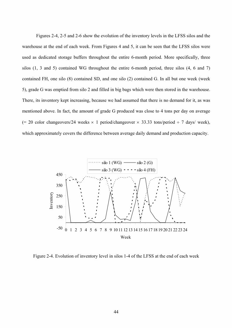
44

Figures 2-4, 2-5 and 2-6 show the evolution of the inventory levels in the LFSS silos and the

warehouse at the end of each week. From Figures 4 and 5, it can be seen that the LFSS silos were

used as dedicated storage buffers throughout the entire 6-month period. More specifically, three

silos (1, 3 and 5) contained WG throughout the entire 6-month period, three silos (4, 6 and 7)

contained FH, one silo (8) contained SD, and one silo (2) contained G. In all but one week (week

5), grade G was emptied from silo 2 and filled in big bags which were then stored in the warehouse.

There, its inventory kept increasing, because we had assumed that there is no demand for it, as was

mentioned above. In fact, the amount of grade G produced was close to 4 tons per day on average

(= 20 color changeovers/24 weeks × 1 period/changeover × 33.33 tons/period ÷ 7 days/ week),

which approximately covers the difference between average daily demand and production capacity.

-50

50

150

250

350

450

0 1 2 3 4 5 6 7 8 9 10 11 12 13 14 15 16 17 18 19 20 21 22 23 24

Week

Inve

ntor

y

silo 1 (WG) silo 2 (G)

silo 3 (WG) silo 4 (FH)

Figure 2-4. Evolution of inventory level in silos 1-4 of the LFSS at the end of each week

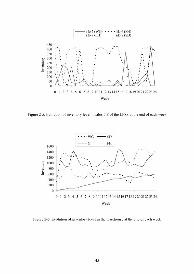
45

050

100150200250300350400450

0 1 2 3 4 5 6 7 8 9 10 11 12 13 14 15 16 17 18 19 20 21 22 23 24

Week

Inve

ntor

y

silo 5 (WG) silo 6 (FH)silo 7 (FH) silo 8 (SD)

Figure 2-5. Evolution of inventory level in silos 5-8 of the LFSS at the end of each week

0200400600800

1000120014001600

0 1 2 3 4 5 6 7 8 9 10 1112 13 14 15 1617 18 19 20 2122 23 24

Week

Inve

ntor

y

WG SD

G FH

Figure 2-6. Evolution of inventory level in the warehouse at the end of each week

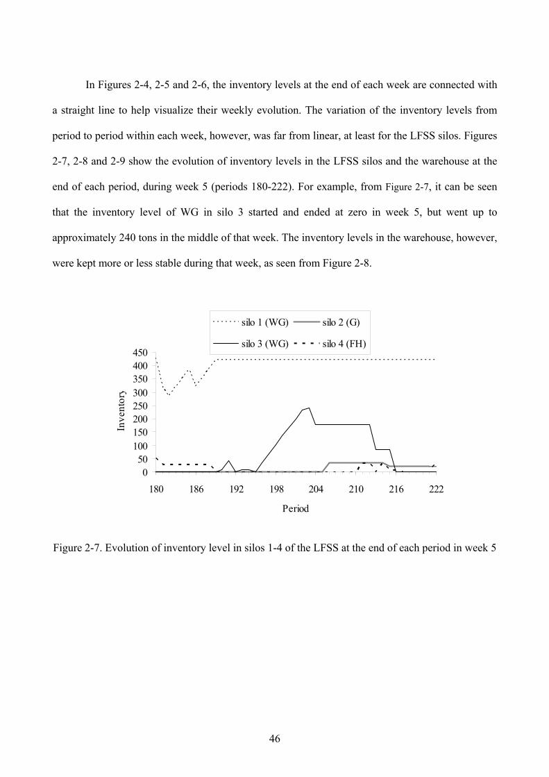
46

In Figures 2-4, 2-5 and 2-6, the inventory levels at the end of each week are connected with

a straight line to help visualize their weekly evolution. The variation of the inventory levels from

period to period within each week, however, was far from linear, at least for the LFSS silos. Figures

2-7, 2-8 and 2-9 show the evolution of inventory levels in the LFSS silos and the warehouse at the

end of each period, during week 5 (periods 180-222). For example, from Figure 2-7, it can be seen

that the inventory level of WG in silo 3 started and ended at zero in week 5, but went up to

approximately 240 tons in the middle of that week. The inventory levels in the warehouse, however,

were kept more or less stable during that week, as seen from Figure 2-8.

050

100150200250300350400450

180 186 192 198 204 210 216 222

Period

Inve

ntor

y

silo 1 (WG) silo 2 (G)

silo 3 (WG) silo 4 (FH)

Figure 2-7. Evolution of inventory level in silos 1-4 of the LFSS at the end of each period in week 5

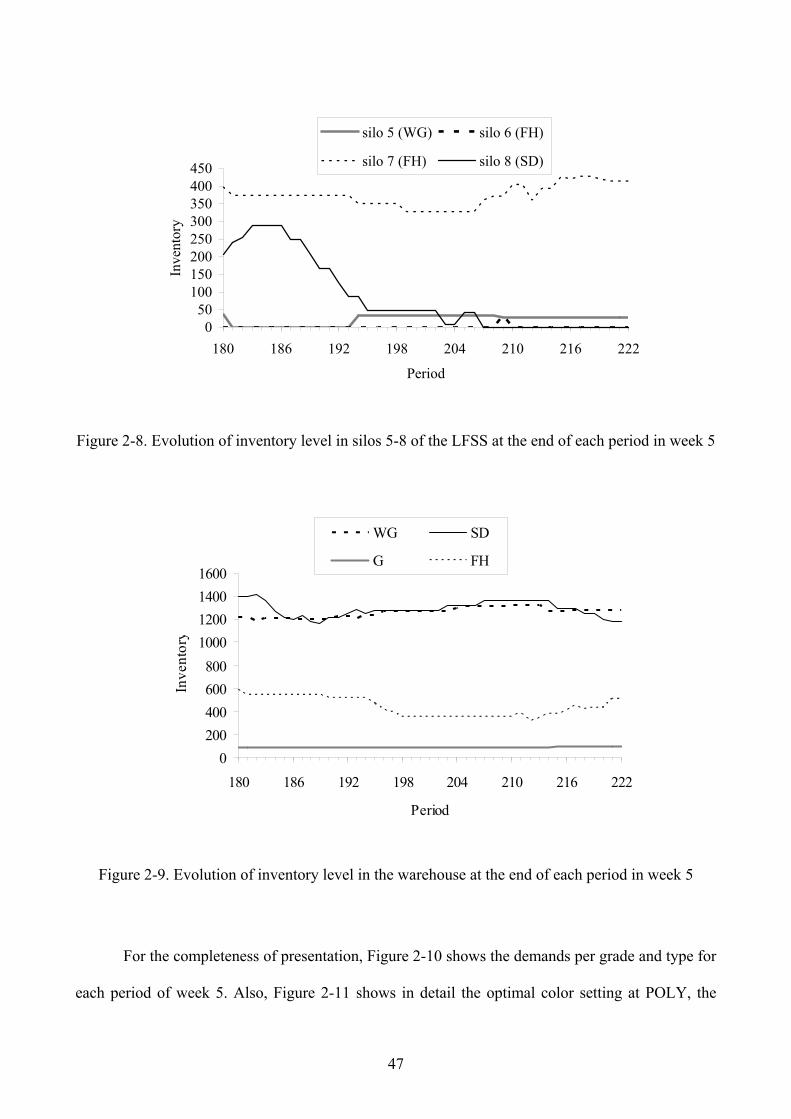
47

050

100150200250300350400450

180 186 192 198 204 210 216 222

Period

Inve

ntor

y

silo 5 (WG) silo 6 (FH)

silo 7 (FH) silo 8 (SD)

Figure 2-8. Evolution of inventory level in silos 5-8 of the LFSS at the end of each period in week 5

0200400600800

1000120014001600

180 186 192 198 204 210 216 222

Period

Inve

ntor

y

WG SD

G FH

Figure 2-9. Evolution of inventory level in the warehouse at the end of each period in week 5

For the completeness of presentation, Figure 2-10 shows the demands per grade and type for

each period of week 5. Also, Figure 2-11 shows in detail the optimal color setting at POLY, the

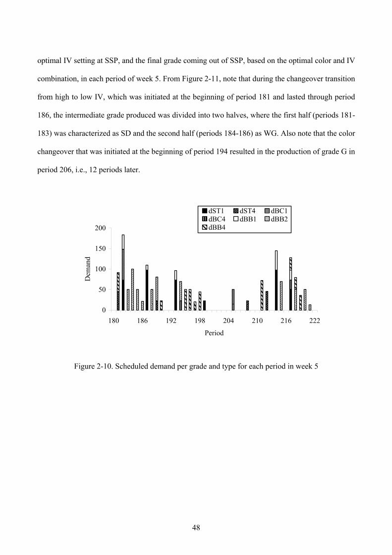
48

optimal IV setting at SSP, and the final grade coming out of SSP, based on the optimal color and IV

combination, in each period of week 5. From Figure 2-11, note that during the changeover transition

from high to low IV, which was initiated at the beginning of period 181 and lasted through period

186, the intermediate grade produced was divided into two halves, where the first half (periods 181-

183) was characterized as SD and the second half (periods 184-186) as WG. Also note that the color

changeover that was initiated at the beginning of period 194 resulted in the production of grade G in

period 206, i.e., 12 periods later.

0

50

100

150

200

180 186 192 198 204 210 216 222

Period

Dem

and

dST1 dST4 dBC1dBC4 dBB1 dBB2dBB4

Figure 2-10. Scheduled demand per grade and type for each period in week 5

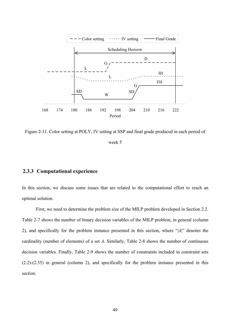
49

168 174 180 186 192 198 204 210 216 222Period

Color setting IV setting Final Grade

DG

LHI

LFH

SDW

G SD

Scheduling Horizon

Figure 2-11. Color setting at POLY, IV setting at SSP and final grade produced in each period of

week 5

2.3.3 Computational experience

In this section, we discuss some issues that are related to the computational effort to reach an

optimal solution.

First, we need to determine the problem size of the MILP problem developed in Section 2.2.

Table 2-7 shows the number of binary decision variables of the MILP problem, in general (column

2), and specifically for the problem instance presented in this section, where “|A|” denotes the

cardinality (number of elements) of a set A. Similarly, Table 2-8 shows the number of continuous

decision variables. Finally, Table 2-9 shows the number of constraints included in constraint sets

(2.2)-(2.35) in general (column 2), and specifically for the problem instance presented in this

section.

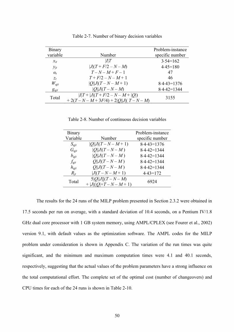
50

Table 2-7. Number of binary decision variables

Binary variable

Number

Problem-instance specific number

xit |I|T 3⋅54=162 yjt |J|(T + F/2 – N – M) 4⋅45=180 αt T – N – M + F – 1 47 zt T + F/2 – N – M + 1 46

Wqjt |Q||J|(T – N – M + 1) 8⋅4⋅43=1376 gqjt |Q||J|(T – N – M) 8⋅4⋅42=1344

Total |I|T + |J|(T + F/2 – N – M + |Q|) + 2(T – N – M + 3F/4) + 2|Q||J|( T – N – M) 3155

Table 2-8. Number of continuous decision variables

Binary Variable

Number

Problem-instance specific number

Sqjt |Q||J|(T – N – M + 1) 8⋅4⋅43=1376 Gqjt |Q||J|(T – N – M ) 8⋅4⋅42=1344 bqjt |Q||J|(T – N – M ) 8⋅4⋅42=1344 fqjt Q||J|(T – N – M ) 8⋅4⋅42=1344 hqjt Q||J|(T – N – M ) 8⋅4⋅42=1344 Rjt |J|(T – N – M + 1) 4⋅43=172

Total 5|Q||J|[(T – N – M) + |J|(|Q|+T – N – M + 1) 6924

The results for the 24 runs of the MILP problem presented in Section 2.3.2 were obtained in

17.5 seconds per run on average, with a standard deviation of 10.4 seconds, on a Pentium IV/1.8

GHz dual core processor with 1 GB system memory, using AMPL/CPLEX (see Fourer et al., 2002)

version 9.1, with default values as the optimization software. The AMPL codes for the MILP

problem under consideration is shown in Appendix C. The variation of the run times was quite

significant, and the minimum and maximum computation times were 4.1 and 40.1 seconds,

respectively, suggesting that the actual values of the problem parameters have a strong influence on

the total computational effort. The complete set of the optimal cost (number of changeovers) and

CPU times for each of the 24 runs is shown in Table 2-10.

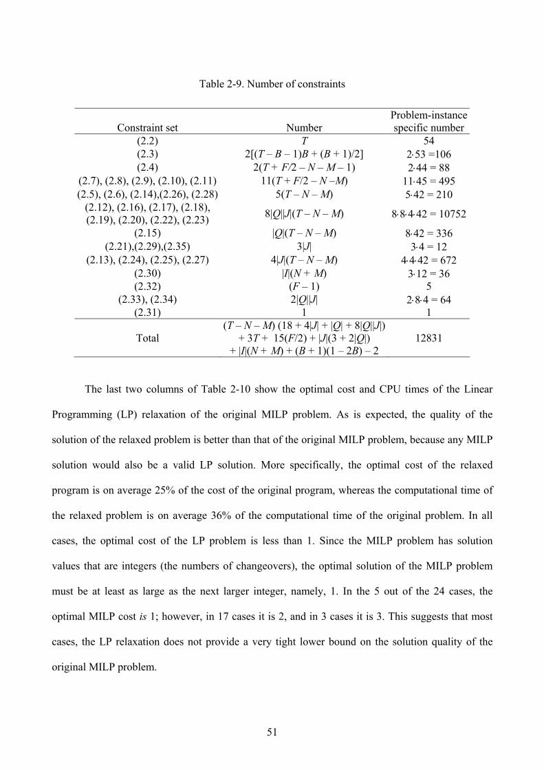
51

Table 2-9. Number of constraints

Constraint set

Number Problem-instancespecific number

(2.2) T 54 (2.3) 2[(T – B – 1)B + (B + 1)/2] 2⋅53 =106 (2.4) 2(T + F/2 – N – M – 1) 2⋅44 = 88

(2.7), (2.8), (2.9), (2.10), (2.11) 11(T + F/2 – N –M) 11⋅45 = 495 (2.5), (2.6), (2.14),(2.26), (2.28) 5(T – N – M) 5⋅42 = 210

(2.12), (2.16), (2.17), (2.18), (2.19), (2.20), (2.22), (2.23) 8|Q||J|(T – N – M) 8⋅8⋅4⋅42 = 10752

(2.15) |Q|(T – N – M) 8⋅42 = 336 (2.21),(2.29),(2.35) 3|J| 3⋅4 = 12

(2.13), (2.24), (2.25), (2.27) 4|J|(T – N – M) 4⋅4⋅42 = 672 (2.30) |I|(N + M) 3⋅12 = 36 (2.32) (F – 1) 5

(2.33), (2.34) 2|Q||J| 2⋅8⋅4 = 64 (2.31) 1 1

Total (T – N – M) (18 + 4|J| + |Q| + 8|Q||J|)

+ 3T + 15(F/2) + |J|(3 + 2|Q|) + |I|(N + M) + (B + 1)(1 – 2B) – 2

12831

The last two columns of Table 2-10 show the optimal cost and CPU times of the Linear

Programming (LP) relaxation of the original MILP problem. As is expected, the quality of the

solution of the relaxed problem is better than that of the original MILP problem, because any MILP

solution would also be a valid LP solution. More specifically, the optimal cost of the relaxed

program is on average 25% of the cost of the original program, whereas the computational time of

the relaxed problem is on average 36% of the computational time of the original problem. In all

cases, the optimal cost of the LP problem is less than 1. Since the MILP problem has solution

values that are integers (the numbers of changeovers), the optimal solution of the MILP problem

must be at least as large as the next larger integer, namely, 1. In the 5 out of the 24 cases, the

optimal MILP cost is 1; however, in 17 cases it is 2, and in 3 cases it is 3. This suggests that most

cases, the LP relaxation does not provide a very tight lower bound on the solution quality of the

original MILP problem.

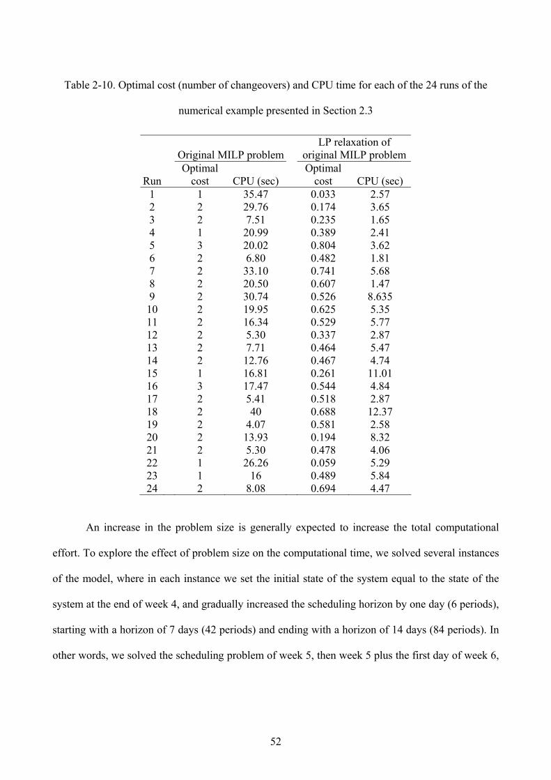
52

Table 2-10. Optimal cost (number of changeovers) and CPU time for each of the 24 runs of the

numerical example presented in Section 2.3

Original MILP problemLP relaxation of

original MILP problem

Run Optimal

cost CPU (sec) Optimal

cost

CPU (sec) 1 1 35.47 0.033 2.57 2 2 29.76 0.174 3.65 3 2 7.51 0.235 1.65 4 1 20.99 0.389 2.41 5 3 20.02 0.804 3.62 6 2 6.80 0.482 1.81 7 2 33.10 0.741 5.68 8 2 20.50 0.607 1.47 9 2 30.74 0.526 8.635 10 2 19.95 0.625 5.35 11 2 16.34 0.529 5.77 12 2 5.30 0.337 2.87 13 2 7.71 0.464 5.47 14 2 12.76 0.467 4.74 15 1 16.81 0.261 11.01 16 3 17.47 0.544 4.84 17 2 5.41 0.518 2.87 18 2 40 0.688 12.37 19 2 4.07 0.581 2.58 20 2 13.93 0.194 8.32 21 2 5.30 0.478 4.06 22 1 26.26 0.059 5.29 23 1 16 0.489 5.84 24 2 8.08 0.694 4.47

An increase in the problem size is generally expected to increase the total computational

effort. To explore the effect of problem size on the computational time, we solved several instances

of the model, where in each instance we set the initial state of the system equal to the state of the

system at the end of week 4, and gradually increased the scheduling horizon by one day (6 periods),

starting with a horizon of 7 days (42 periods) and ending with a horizon of 14 days (84 periods). In

other words, we solved the scheduling problem of week 5, then week 5 plus the first day of week 6,

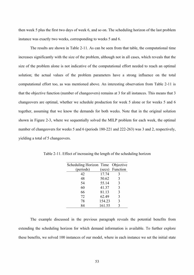
53

then week 5 plus the first two days of week 6, and so on. The scheduling horizon of the last problem

instance was exactly two weeks, corresponding to weeks 5 and 6.

The results are shown in Table 2-11. As can be seen from that table, the computational time

increases significantly with the size of the problem, although not in all cases, which reveals that the

size of the problem alone is not indicative of the computational effort needed to reach an optimal

solution; the actual values of the problem parameters have a strong influence on the total

computational effort too, as was mentioned above. An interesting observation from Table 2-11 is

that the objective function (number of changeovers) remains at 3 for all instances. This means that 3

changeovers are optimal, whether we schedule production for week 5 alone or for weeks 5 and 6

together, assuming that we know the demands for both weeks. Note that in the original solution

shown in Figure 2-3, where we sequentially solved the MILP problem for each week, the optimal

number of changeovers for weeks 5 and 6 (periods 180-221 and 222-263) was 3 and 2, respectively,

yielding a total of 5 changeovers.

Table 2-11. Effect of increasing the length of the scheduling horizon

Scheduling Horizon(periods)

Time(secs)

ObjectiveFunction

42 17.74 3 48 50.62 3 54 55.14 3 60 41.37 3 66 81.13 3 72 62.49 3 78 154.23 3 84 161.55 3

The example discussed in the previous paragraph reveals the potential benefits from

extending the scheduling horizon for which demand information is available. To further explore

these benefits, we solved 100 instances of our model, where in each instance we set the initial state

54

of the system equal to the state of the system at the end of week 4, the scheduling horizon equal to 2

weeks, and the demand in the first week equal to the demand in week 5. In each instance, the

demand in week 6 was randomly generated from a distribution which we constructed based on the

demands over the 6-month period for which we had data. One of the things we wanted to examine

by running this experiment was the sensitivity of the cost (number of changeovers) in the first week

with respect to the demand realizations in the second week, when we choose to solve the scheduling

problem for weeks 5 and 6 as a single 2-week problem instead of two 1-week problems. We also

wanted to see how the solution of the 2-week problem compared to the sum of the solutions of the

two sequential 1-week problems.

The results are presented in Appendix B. They suggest that if demand data is available for

two weeks instead of one week ahead of time, the chemical plant can be scheduled much more

efficiently, i.e. with significantly fewer changeovers. This is because when the demand of the

second week is known in advance, the scheduling procedure has the opportunity to merge the

production of different quantities of the same grade, if possible, so as to decrease the total number

of needed changeovers. As is expected, solving the single 2-week problem requires a longer

computational time generally than solving the two 1-week problems. However, there exist some

instances in which the required computational time for solving the scheduling problem of the

second week as a single 1-week scheduling problem is longer than the required computational time

for solving the respective 2-week problem. This is attributed to the fact that the required

computational time strongly depends on the relevant position of initial final grades inventories and

the emerging demand, because in case of a “tighter” respective situation, the optimization procedure

has to search the optimal solution in a more rough solution space.

55

2.4 Conclusions

We developed an MILP model for the production scheduling of a multi-grade PET processing

chemical plant. We also presented an application of the model on a real case study, along with some

discussion that provides insight into its behavior. The model minimizes the cost associated with the

number of grade changeovers, while also ensuring that the capacity constraints of the problem are

not violated and that the demand for final products is satisfied on time. The model incorporates all

aspects of the problem under consideration and can be easily extended to address additional ones

that may arise in different situations, because of the large number of decision variables that

enhances its flexibility. We believe that the main contribution of this work is that it addresses

efficiently an important practical application, whose solution exhibits high complexity.

56

57

Chapter 3 The stochastic economic lot sizing

problem for continuous nonstop

multi-grade production

In this chapter, we study a variant of the Stochastic Economic Lot Scheduling problem (SELSP) in

which a single production facility must produce several different grades of a family of products to

meet random stationary demand for each grade from a common Finished-Goods (FG) inventory

buffer with limited storage capacity. Demand that can not be satisfied directly from inventory is

lost. Raw material is always available, and the production facility produces continuously at a

constant rate. When the facility is set up to produce a particular grade, the only allowable

changeovers are from that grade to the next lower or higher grade. All changeover times are

constant and equal to each other. There is a changeover cost per changeover occasion, a spill-over

cost per unit of product in excess whenever there is not enough space in the FG buffer to store the

produced grade, and a lost-sales cost per unit short whenever there is not enough FG inventory to

satisfy the demand. We model the SELSP as a discrete-time Markov Decision Process (MDP),

where in each time period the decision is whether to initiate a changeover to a neighboring grade or

keep the set up of the production facility unchanged, based on the current state of the system which

is defined by the current set up of the facility and the FG inventory levels of all the grades. The goal

58

is to minimize the (long-run) expected average cost per period. For 2- and 3-grade problems, we

numerically solve the exact MDP problem using the value iteration method. For problems with

more than three grades, we develop a heuristic solution procedure which is based on approximating

the original multi-grade problem with several 3-grade sub-problems and numerically solving each

sub-problem using value iteration. We present numerical results for problem examples with 2-5

grades. For the 2- and 3-grade examples, we use the exact solution procedure to obtain insights into

the structure of the optimal changeover policy. For the 4- and 5-grade examples, we compare the

performance of the heuristic solution procedure against that of the exact procedure.

3.1 Introduction

Scheduling production of multiple products, each with random demand, on a single facility with

limited production capacity and significant changeover costs and times between products is a

classic problem in production planning research that is often referred to as the Stochastic Lot

Scheduling Problem (SLSP). Sox et al. (1999) distinguish between two versions of the SLSP, for

consistency with the deterministic-demand literature: the Stochastic Capacitated Lot Sizing Problem

(SCLSP) and the Stochastic Economic Lot Sizing Problem (SELSP). The SCLSP assumes a finite

planning horizon and allows for non-stationary demand, while the SELSP assumes an infinite

planning horizon and stationary demand. The SCLSP is more appropriate for discrete-parts

manufacturing, whereas the SELSP is perhaps better suited for continuous-processing

manufacturing. Discrete-parts manufacturing is characterized by individual parts that are clearly

distinguishable, and is often encountered in the industries of computer and electronic products,

electrical equipment and appliances, transport equipment, machinery, fabricated metal, wood,

furniture products, etc. Process industries, on the other hand, operate on material that is

continuously flowing, as is the case with petroleum and coal products, metallurgical products,

59

nonmetallic mineral products, basic chemicals, food and beverage products, paper products, etc.

Generally, process industries are capital intensive and focus on high-volume, low-variety

production. In a typical process industry, the production facility produces continuously, at a

constant rate, and the different products are really variants of the same family that differ in one or

more attributes, such as quality, color, consistency, weight, size, thickness, etc. These variants are

frequently referred to as “grades”. Often, the different grades are related in such a way that the only

allowable changeovers are from one grade to the next higher or lower grade in the chain. For

example, if the facility produces three grades, A, B, and C (A being the lowest and C being the

highest), the allowable changeovers are between A and B, between B and C, but not directly

between A and C. To indicate this ordering in the chain of allowable changeovers, we use the

notation “A-B-C”. Avoiding grade changeovers is often of primary managerial concern, because

during a changeover transition, the process is difficult to control, and the grade produced is off-

specifications.

The deterministic version of the SELSP, the so-called ELSP, has received considerable

attention in the literature over the past decades (e.g., see the surveys of Elmaghraby, 1978 and

Salomon, 1991). Both analytical and heuristic solutions for the ELSP derive rigid cyclic production

plans, which in many multi-grade plants take the form of rigid product slates or wheels, whereby all

grades are produced sequentially in a cycle, starting from the lowest grade, going up all the way to

the highest grade, and returning down to the lowest grade. In the previous example with the three

grades, a complete grade slate would be A→B→C→B→A. Interestingly, clearing policies, i.e.,

policies where the facility switches to the product whose inventory level reaches zero first, may lead

to inventory trajectories that exhibit chaotic behavior, i.e., that are sensitive to initial conditions, are

non-periodic, etc., as Chase et al. (1993) show, even for a 3-product system with no changeover

times and no constraints on the order of allowable changeovers.

60

Unfortunately, cyclic plans do not work well for the stochastic problem, for two reasons.

Firstly, they focus on lot-sizing and not on dynamic capacity allocation, which is necessary to

respond to random changes in demand. Secondly, in the stochastic problem, finished-goods (FG)

inventories serve not only to reduce the number of changeovers, as is the case in the deterministic

problem, but also to hedge against stock-outs. In the stochastic problem, both lot-sizing and

capacity allocation have to be considered simultaneously, and the dynamics have to be included in

the plan (Graves, 1980).

In this chapter, we study a variant of the SELSP in which a single production facility must

produce several grades to meet random stationary demand for each grade from a common FG

inventory buffer with limited storage capacity. Demand that can not be satisfied directly from stock

is lost. Raw material is always available, and the production facility produces at a constant rate all

the time. When the facility is set up to produce a particular grade, the only allowable changeovers

are from that grade to the next lower or higher grade. In many industries, it is customary to divide

the intermediate grade produced during a changeover, say from grade A to grade B, into two halves,

and classify the first half as A and the second half as B, although in reality the grade of the product

coming out of the production facility during the changeover transition is gradually changing from A

to B. In this chapter, for simplicity, we assume that the grade produced during a changeover from A

to B is classified as A, and that the grade produced during the reverse changeover is classified as B.

Under this assumption, the amounts of grades A and B that will be produced in the long run will be

the same as those that would have been produced had we divided the produced grade during a

changeover into two halves. We also assume that all changeover times are deterministic and equal

to each other.

The cost structure of our model includes a changeover cost per changeover occasion, a spill-

over cost per unit of product in excess whenever there is not enough space in the FG buffer to store

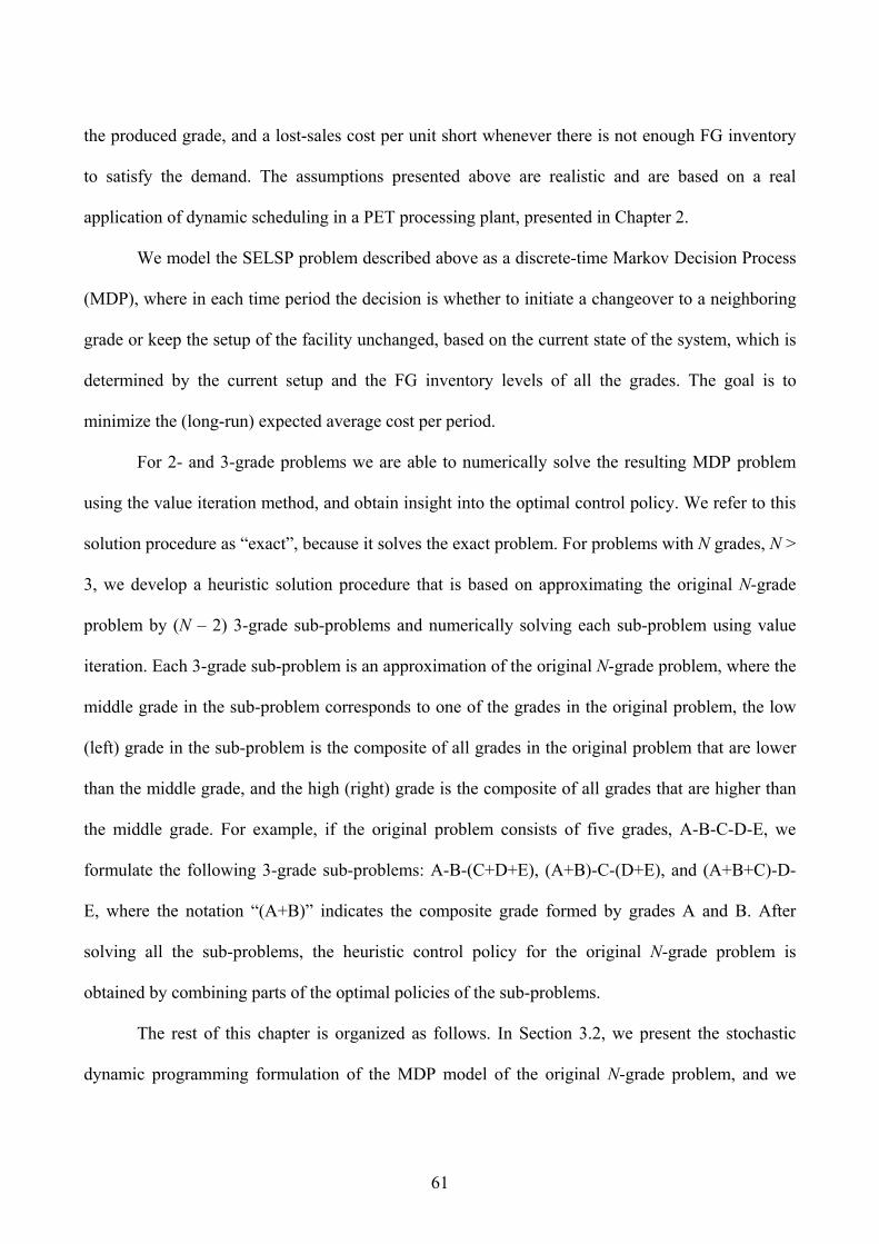
61

the produced grade, and a lost-sales cost per unit short whenever there is not enough FG inventory

to satisfy the demand. The assumptions presented above are realistic and are based on a real

application of dynamic scheduling in a PET processing plant, presented in Chapter 2.

We model the SELSP problem described above as a discrete-time Markov Decision Process

(MDP), where in each time period the decision is whether to initiate a changeover to a neighboring

grade or keep the setup of the facility unchanged, based on the current state of the system, which is

determined by the current setup and the FG inventory levels of all the grades. The goal is to

minimize the (long-run) expected average cost per period.

For 2- and 3-grade problems we are able to numerically solve the resulting MDP problem

using the value iteration method, and obtain insight into the optimal control policy. We refer to this

solution procedure as “exact”, because it solves the exact problem. For problems with N grades, N >

3, we develop a heuristic solution procedure that is based on approximating the original N-grade

problem by (N – 2) 3-grade sub-problems and numerically solving each sub-problem using value

iteration. Each 3-grade sub-problem is an approximation of the original N-grade problem, where the

middle grade in the sub-problem corresponds to one of the grades in the original problem, the low

(left) grade in the sub-problem is the composite of all grades in the original problem that are lower

than the middle grade, and the high (right) grade is the composite of all grades that are higher than

the middle grade. For example, if the original problem consists of five grades, A-B-C-D-E, we

formulate the following 3-grade sub-problems: A-B-(C+D+E), (A+B)-C-(D+E), and (A+B+C)-D-

E, where the notation “(A+B)” indicates the composite grade formed by grades A and B. After

solving all the sub-problems, the heuristic control policy for the original N-grade problem is

obtained by combining parts of the optimal policies of the sub-problems.

The rest of this chapter is organized as follows. In Section 3.2, we present the stochastic

dynamic programming formulation of the MDP model of the original N-grade problem, and we

62

outline the successive approximation method to solve it. The heuristic procedure for solving

problems with more than three grades is presented in Section 3.3. In Section 3.4, we present

numerical results for problem examples with 2-5 grades. For the 2- and 3-grade examples, we use

the exact solution procedure to obtain insights into the structure of the optimal changeover policy.

For the 4- and 5-grade examples, we compare the performance of the heuristic solution procedure

against that of the exact procedure. Finally, we draw our conclusions in Section 3.5.

3.2 Problem formulation and dynamic programming solution

We consider a discrete-time model of a production facility that can produce N different grades, one

at a time. Grade changeovers are only allowed between neighboring grades, n and n + 1, n = 1, …,

N – 1. The changeover time is one period. In each time period, the production facility produces P

units of the grade that it is set up for at the beginning of the period. The quantity produced is stored

in a common FG inventory buffer which has a finite storage capacity of X units; any excess amount

that does not fit in the buffer is spilled over, incurring a spill-over cost of CS dollars per unit of

excess product. The FG buffer is flexible in that it can contain any quantity of any grade at the same

time, as long as the total amount does not exceed X. After the quantity produced by the facility has

been added to the FG buffer, a vector of random demands, D ≡ (D1, …, DN), must be met from FG

inventory, where Dn, n = 1, …, N, is the demand for grade n. The demands Dn are discrete random

variables with known stationary joint probability distribution. For each grade n, the part of the

demand that can not be satisfied from FG inventory, if any, is lost, incurring a lost-sales cost of CLn

dollars per unit of unsatisfied demand. In many real problems, especially in the process industries,

changing P may cause instabilities in the production process; therefore, P is not considered to be a

control variable for scheduling purposes, but is finely re-tuned once in a while so as to match the

total expected demand for all grades, in case the demand has seasonal or other long-term variations.

63

For the purposes of short- to medium-term scheduling that we consider in this chapter, we assume

that P is fixed and equal to the total expected demand for all grades.

We formulate the dynamic scheduling problem of the production facility as a discrete-time

MDP, where the state of the system at the beginning of each period is defined by the vector y ≡ (s,

x1, …, xN), where s is the grade that the facility is set up for during that period (called the “setup”

state) and xn, n = 1, …, N, is the FG inventory level of grade n at the beginning of the period. Note

that s ∈ 1, …, N, and the set of allowable inventory levels is determined by all integers xn, n = 1,

…, N, such that 0 ≤ Σn xn ≤ X. It is easy to see that the size of the state space is (N⋅XN)/2.

The decision, u, to be made at the beginning of each period is whether to initiate a

changeover to a neighboring grade or leave the facility setup unchanged. Thus, if the current setup

is s, the allowable decisions are given by the set U(s), where U(1) = 1, 2, U(s) = s – 1, s, s + 1,

s = 2, …, N – 1, and U(N) = N – 1, N. If the decision is to initiate a changeover, then the new

setup of the facility, i.e., after the changeover is completed, will be in effect at the beginning of the

next period, since the changeover time is one period. A decision to initiate a changeover at the

beginning of a period incurs a changeover cost of CC dollars in that period.

Suppose that the state of the system at the beginning of a period is y, decision u is taken, and

demand D is realized. Let g(y,u,D) be the cost incurred during that period and let y′ ≡ (s′, x1′, …,

xN′) = f(y,u,D) be the state of the system at the beginning of the next period. From the above

discussion, it is clear that

s′ = u

xn′ = (xn + p(y)⋅In=s – Dn)+, n = 1, …, N

where p(y) is the amount added to the FG buffer after the facility produces P units and before the

demand is satisfied and is given by p(y) ≡ min(P, X – Σn xn), Ia is the indicator function which takes

the value of 1 if a is true, and 0 otherwise, and (x)+ ≡ max(0, x). Moreover,

64

g(y,u,D) = CC⋅Iu≠s + CS⋅(P – p(y)) + Σn CLn⋅(Dn – xn – p(y)⋅In=s)+

The objective is to find a state dependent policy, u = μ(y), that minimizes the (long-run)

expected average cost per period. To find such a policy, we need to solve Bellman’s dynamic

programming equation, which for our problem can be written as

J + V(y) = minu∈U(s)Tu(V(y)) (3.1)

where J is the optimal (minimum) expected average cost per period, V(y) is the optimal differential

cost starting from state y, and Tu(⋅) is a mapping defined as Tu(V(y)) ≡ EDg(y,u,D) + V(y′). The

minimizer of the Bellman equation determines the optimal policy when the system is in state y,

denoted by μ*(y).

To solve Bellman’s equation, we use the method of successive approximations of the

optimal differential cost functions, which is known as the value iteration method. We denote by

Vk(y) the value of the optimal differential cost function at the kth iteration. Initially, we set V0(y) =

0, ∀ y. The values at the (k + 1)th iteration are obtained from the previous iteration by the recursion

Vk+1(y) = T(Vk(y)) – T(Vk(ŷ)) (3.2)

where T(Vk(y)) = minu∈U(s)Tu(Vk(y)) and ŷ is an arbitrarily chosen special state. Note that in each

iteration the optimal differential cost of the special state is reset to zero. Assuming that the iteration

scheme converges to some values V(y), then from recursion (3.2), these values must satisfy T(V(ŷ))

+ V(y) = T(V(y)). A comparison of this equation and the Bellman equation (3.1) reveals that J =

T(V(ŷ)).

To implement the successive approximation method, at each iteration k = 1, 2, … we

compute the maximum and minimum differences, VkU = maxyVk(y) – Vk–1(y) and Vk

L =

minyVk(y) – Vk–1(y). The procedure is terminated when |VkU – Vk

L| < ε⋅T(Vk(ŷ)), where ε is some

small positive scalar.

65

3.3 Heuristic solution procedure

Although the exact method presented in the preceding section can in principle determine the

optimal policy for any number of grades, it becomes computationally intractable for more than three

grades. In this section, we propose a heuristic procedure that approximates any N-grade problem, N

> 3, by several 3-grade sub-problems and then uses the sub-problem solutions (determined by the

exact method) to construct a heuristic policy for the original problem.

The heuristic procedure that we propose works as follows. Let S denote the original N-grade

problem. For each grade n, n = 2, …, N – 1, we formulate a 3-grade sub-problem, denoted by Sn, in

which the middle grade is grade n, the low grade is the composite of all grades that are lower than n,

i.e., grades 1, …, n – 1, and the high grade is the composite of all grades that are higher than n, i.e.,

grades n + 1, …, N; hence Sn is an approximation of the original problem S. For each sub-problem

Sn, we define the state of the system by the vector yn = (sn, wn, xn, zn), where sn ∈ 1, 2, 3 and wn

and zn are the inventory levels of the low and high composite grades, respectively, and are given by

the sums: wn ≡ x1 + … + xn–1 and zn ≡ xn+1 + … + xN. In each sub-problem Sn, the demand

distribution of the middle grade is the same as the demand distribution of grade n in the original

problem, the demand distribution of the low grade is the convolution of the demand distributions of

grades 1, …, n – 1 in the original problem, and the demand distribution of the high grade is the

convolution of the demand distributions of grades n + 1, …, N in the original problem.

We use the exact method presented in the previous section to obtain the optimal policy of

sub-problem Sn, denoted by μn*(yn). The heuristic policy for the original N-grade problem, denoted

by μh(y), is then constructed by using parts of the optimal policies of the sub-problems, as follows:

μh(1, x1, …, xN) = μ2*(1, ŵ2, x2, ž2)

μh(n, x1, …, xN) = μn*(2, ŵn, xn, žn) + n – 2, n = 2, …, N – 1

66

μh(N, x1, …, xN) = μN–1*(3, ŵN–1, xN–1, žN–1) + N – 3

where ŵn and žn are the “aggregate” inventory levels of the low and high composite grades,

respectively, in sub-problem Sn, which represent in some aggregate way the total of their individual

components through some function h, i.e., ŵn = h(x1, …, xn–1) and žn = h(xn+1, …, xn). The terms “n

– 2” and “N – 3” on the right-hand side of two of the above expressions are correction terms that

account for the fact that setup states 1, 2, and 3 in sub-problem Sn, n = 2, …, N – 1, correspond to

setup states n – 1, n, and n + 1, respectively, in the original problem. Next, we discuss how to

determine an appropriate form for function h.

First, note that ŵ2 = h(x1), i.e., ŵ2 is the aggregate inventory level of a single grade, namely

grade 1; therefore, it is reasonable to simply set h(x1) ≡ x1 so that ŵ2 = h(x1) = x1. Similarly, we set

h(xN) ≡ xN, so that žN–1 = h(xN) = xN. Let us next focus on ŵn, n > 2, as žn is obtained in exactly the

same way.

An obvious choice for the aggregate inventory level of the composite of grades 1, …, n – 1

is to set it equal to the sum of the inventory levels of the individual grades, i.e., set ŵn = wn. This is

a reasonable choice, especially with respect to estimating potential spill-over costs, but fails to

detect the situation where the sum wn is high, implying that the composite grade has a low risk of

stock-out, but one (or more) of its individual components, x1, …, xn–1, is (are) low, implying that the

corresponding individual grade(s) has(ve) a high risk of stock-out, which may lead to significant

lost-sales costs. We refer to this situation as the “imbalance problem,” because one or more of the

individual inventory levels are much lower than the average.

To illustrate the imbalance problem, suppose that the facility is currently set up to produce

grade 4, and that the inventory levels of grades 1-4 are (x1, x2, x3, x4) = (15, 15, 0, 6). Then, in sub-

problem S4, the inventory level of the middle grade would be x4 = 6, and the total inventory level of

the low composite grade would be w4 = x1 + x2 + x3 = 30. In this case, the optimal policy obtained

67

from solving S4 might indicate that it is optimal for the facility not to change over to the low

composite grade, because there is plenty of it (30 units) in storage compared to the inventory level

of the middle grade 4, which is much lower (6 units). What the heuristic fails to see here is that

although w4 is relatively high, its individual components are quite imbalanced – in fact, one of

them, namely x3, is zero. In this case, unless the facility changes over to grade 3, a heavy lost-sales

cost is likely to be incurred in the current and in the following period.

To tackle the imbalance problem, we seek an aggregate inventory level, ŵn, for the

composite of grades 1, …, n – 1, that would somehow reflect the imbalance, if any, among the

individual inventory levels x1, …, xn–1. A natural measure of the imbalance of the individual

inventory levels is the sum of their expected lost sales, denoted by ILSn, given by

ILSn ≡ E[(D1 – x1)+] + … + E[(Dn–1 – xn–1)+]

The expected lost sales for any given aggregate inventory level, w, of the composite grade, on the

other hand, denoted by CLSn(w), is given by

CLSn(w) ≡ E[(D1 + … + Dn–1 – w)+]

With the above definitions in mind, in order to capture the imbalance, if any, among the

individual inventory levels x1, …, xn–1, we propose the following expression for the aggregate

inventory level, ŵn:

, if 0

ˆ, if 0

n nn

n n

w ILSw

v ILS=⎧

= ⎨ >⎩ (3.3)

where vn ≡ w: CLSn(w) = ILSn, i.e., vn is that value of the aggregate inventory level which makes the

expected lost sales of the composite grade equal to the sum of the expected lost sales of the

individual grades.

To compute vn we need to derive the probability distribution of the demand of the composite

grade by convolving the probability distributions of the demands of the individual grades. In case

68

this is not computationally convenient, we propose a faster alternative in which we approximate

ILSn by the expression

ILSn ≈ (E[D1] – x1)+ + … + (E[Dn–1] – xn–1)+

This then allows us to compute vn by the following expression:

vn = E[D1] + … + E[Dn–1] – ILSn (3.4)

Expression (3.3) prescribes that the aggregate inventory level, ŵn, be set equal to either wn,

if ILSn = 0, or vn, if ILSn > 0. It can be easily shown that vn ≤ wn. Given that vn may be significantly

smaller than wn, where wn is the natural candidate for the aggregate inventory level of the composite

grade, we propose to use a “smoother”, more general rule than the one prescribed by expression

(3.3). According to the more general rule, ŵn is set equal to a linear combination of wn and vn

(rounded to the nearest integer), if ILSn > 0, namely

, if 0

ˆ(1 ) , if 0

n nn

n n n

w ILSw

v w ILSα α=⎧

= ⎨ + − >⎩ (3.5)

for some coefficient α, such that 0 ≤ α ≤ 1, where vn is given by (3.4). Note that if α = 0, the rule

prescribed by (3.5) becomes ŵn = wn, whereas if α = 1, the rule becomes identical to that prescribed

by expression (3.3). Clearly, the smaller the imbalance problem, the smaller the optimal value of α,

and the better the performance of the heuristic. In Section 3.4.3, we investigate the performance of

the heuristic as a function of coefficient α.

The heuristic policy that we described above, as any feedback policy, satisfies an expression

similar to Bellman’s equation (3.1), without the minimization, i.e., it satisfies

( ) ( ( ))hh h h

uJ V T V+ =y y (3.6)

where Jh is the expected average cost per period and Vh(y) is the differential cost starting from state

y, when the heuristic policy uh = μh(y) is used. Note that Jh, Vh(y), and μh(y) also depend on α, but

we omitted this dependence here for notational simplicity.

69

One way to evaluate the heuristic policy is to use the method of successive approximations

of the differential cost functions Vh(y). More specifically, if we denote by ( )hkV y the values of the

differential cost function at the kth iteration, then the values at the (k + 1)th iteration are obtained

from the previous iteration by a recursion similar to (3.2), without the minimization, i.e.,

1 ˆ( ) ( ( )) ( ( ))h hh h h

k k ku uV T V T V+ = −y y y (3.7)

Note that as in (3.2), at each step of iteration (3.7), the differential cost of the special state ŷ is reset

to zero. Assuming that the iteration scheme converges to some values V(y), for all y, then the

expected average cost per period of the heuristic policy is given by ˆ( ( ))hh h

uJ T V= y .

An alternative way to evaluate the heuristic policy is to use simulation. Our numerical

experience for 4-grade and 5-grade problems showed that the simulation is faster than the method

of successive approximations by as much as 100 times.

3.4 Numerical results

In this section, we present numerical results for problem examples with 2-5 grades. First, we solve a

2-grade example using the exact solution procedure. For that example, we discuss the optimal

changeover policy, and we explore the effect of problem parameters on the optimal expected

average cost per period and on the computational time of the successive approximation procedure.

Then, we solve a 3-grade example originating from a real application presented in Chapter 2, for

which we also discuss the optimal changeover policy. Finally, we solve 4-grade and 5-grade

examples using both the exact and the heuristic solution procedures. We discuss the performance

and computational efficiency of the heuristic procedure, and we explore how they are affected by

the distribution of the relative market size of the different grades and the size of weight α in

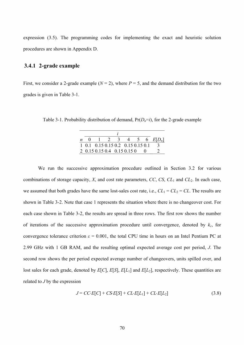
70

expression (3.5). The programming codes for implementing the exact and heuristic solution

procedures are shown in Appendix D.

3.4.1 2-grade example

First, we consider a 2-grade example (N = 2), where P = 5, and the demand distribution for the two

grades is given in Table 3-1.

Table 3-1. Probability distribution of demand, Pr(Dn=i), for the 2-grade example

i n 0 1 2 3 4 5 6 E[Dn]1 0.1 0.15 0.15 0.2 0.15 0.15 0.1 3 2 0.15 0.15 0.4 0.15 0.15 0 0 2

We run the successive approximation procedure outlined in Section 3.2 for various

combinations of storage capacity, X, and cost rate parameters, CC, CS, CL1 and CL2. In each case,

we assumed that both grades have the same lost-sales cost rate, i.e., CL1 = CL2 = CL. The results are

shown in Table 3-2. Note that case 1 represents the situation where there is no changeover cost. For

each case shown in Table 3-2, the results are spread in three rows. The first row shows the number

of iterations of the successive approximation procedure until convergence, denoted by kc, for

convergence tolerance criterion ε = 0.001, the total CPU time in hours on an Intel Pentium PC at

2.99 GHz with 1 GB RAM, and the resulting optimal expected average cost per period, J. The

second row shows the per period expected average number of changeovers, units spilled over, and

lost sales for each grade, denoted by E[C], E[S], E[L1] and E[L2], respectively. These quantities are

related to J by the expression

J = CC⋅E[C] + CS⋅E[S] + CL⋅E[L1] + CL⋅E[L2] (3.8)

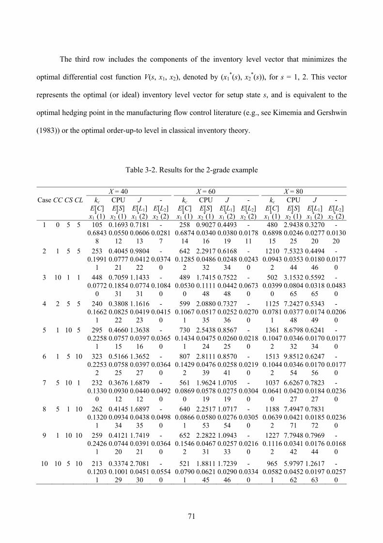
71

The third row includes the components of the inventory level vector that minimizes the

optimal differential cost function V(s, x1, x2), denoted by (x1*(s), x2

*(s)), for s = 1, 2. This vector

represents the optimal (or ideal) inventory level vector for setup state s, and is equivalent to the

optimal hedging point in the manufacturing flow control literature (e.g., see Kimemia and Gershwin

(1983)) or the optimal order-up-to level in classical inventory theory.

Table 3-2. Results for the 2-grade example

X = 40 X = 60 X = 80 Case CC CS CL kc CPU J - kc CPU J - kc CPU J -

Ε[C] E[S] E[L1] E[L2] Ε[C] E[S] E[L1] E[L2] Ε[C] E[S] E[L1] E[L2] x1

*(1) x2*(1) x1

*(2) x2*(2) x1

*(1) x2*(1) x1

*(2) x2*(2) x1

*(1) x2*(1) x1

*(2) x2*(2)

1 0 5 5 105 0.1693 0.7181 - 258 0.9027 0.4493 - 480 2.9438 0.3270 - 0.6843 0.0550 0.0606 0.0281 0.6874 0.0340 0.0380 0.0178 0.6898 0.0246 0.0277 0.0130 8 12 13 7 14 16 19 11 15 25 20 20

2 1 5 5 253 0.4045 0.9804 - 642 2.2917 0.6168 - 1210 7.5323 0.4494 - 0.1991 0.0777 0.0412 0.0374 0.1285 0.0486 0.0248 0.0243 0.0943 0.0353 0.0180 0.0177 1 21 22 0 2 32 34 0 2 44 46 0

3 10 1 1 448 0.7059 1.1433 - 489 1.7415 0.7522 - 502 3.1532 0.5592 - 0.0772 0.1854 0.0774 0.1084 0.0530 0.1111 0.0442 0.0673 0.0399 0.0804 0.0318 0.0483 0 31 31 0 0 48 48 0 0 65 65 0

4 2 5 5 240 0.3808 1.1616 - 599 2.0880 0.7327 - 1125 7.2427 0.5343 - 0.1662 0.0825 0.0419 0.0415 0.1067 0.0517 0.0252 0.0270 0.0781 0.0377 0.0174 0.0206 1 22 23 0 1 35 36 0 1 48 49 0

5 1 10 5 295 0.4660 1.3638 - 730 2.5438 0.8567 - 1361 8.6798 0.6241 - 0.2258 0.0757 0.0397 0.0365 0.1434 0.0475 0.0260 0.0218 0.1047 0.0346 0.0170 0.0177 1 15 16 0 1 24 25 0 2 32 34 0

6 1 5 10 323 0.5166 1.3652 - 807 2.8111 0.8570 - 1513 9.8512 0.6247 - 0.2253 0.0758 0.0397 0.0364 0.1429 0.0476 0.0258 0.0219 0.1044 0.0346 0.0170 0.0177 2 25 27 0 2 39 41 0 2 54 56 0

7 5 10 1 232 0.3676 1.6879 - 561 1.9624 1.0705 - 1037 6.6267 0.7823 - 0.1330 0.0930 0.0440 0.0492 0.0869 0.0578 0.0275 0.0304 0.0641 0.0420 0.0184 0.0236 0 12 12 0 0 19 19 0 0 27 27 0

8 5 1 10 262 0.4145 1.6897 - 640 2.2517 1.0717 - 1188 7.4947 0.7831 0.1320 0.0934 0.0438 0.0498 0.0866 0.0580 0.0276 0.0305 0.0639 0.0421 0.0185 0.0236 1 34 35 0 1 53 54 0 2 71 72 0

9 1 10 10 259 0.4121 1.7419 - 652 2.2822 1.0943 - 1227 7.7948 0.7969 - 0.2426 0.0744 0.0391 0.0364 0.1546 0.0467 0.0257 0.0216 0.1116 0.0341 0.0176 0.0168 1 20 21 0 2 31 33 0 2 42 44 0

10 10 5 10 213 0.3374 2.7081 - 521 1.8811 1.7239 - 965 5.9797 1.2617 - 0.1203 0.1001 0.0451 0.0554 0.0790 0.0621 0.0290 0.0334 0.0582 0.0452 0.0197 0.0257 1 29 30 0 1 45 46 0 1 62 63 0

72

From the results, it can be seen that the values of kc and CPU range from 105 iterations in

0.1693 hours (∼10 min), in case 1 (X = 40), to 1513 iterations in 9.8512 hours, in case 6 (X = 80).

As X increases, kc and CPU increase significantly, whereas E[C], E[S] E[L1], E[L2] and J decrease,

as would be expected. Note that kc and CPU are significantly lower in case 1 than in any other case,

since CC = 0 in case 1. As would also be expected, J increases as the cost rate parameters increase.

From the results, it can also be seen that as one of the cost rate parameters, say CS, increases, the

respective quantity that it multiplies in the objective function (3.8), i.e., E[C], decreases, but the

overall optimal expected average cost per period, J, increases.

In all cases, except case 1, the optimal inventory level of the grade that the facility is set up

for is close to or equal to zero, whereas the optimal inventory level of the other grade is quite

significant. The reason for this is that when the facility is set up for a particular grade, say grade 1,

ideally one would like to have low inventory of grade 1 and high inventory of grade 2, so that the

facility can continue producing grade 1 for as many periods as possible without having to change

over to grade 2 and pay the changeover cost. This is no longer true for case 1, where changeovers

cost nothing.

Also, the optimal inventory levels seem to be more or less symmetric for the two grades,

i.e., x1*(1) ≈ x2

*(2) and x2*(1) ≈ x1

*(2), except that the inventory level of grade 1 is slightly higher

than that of grade 2, because grade 1 has higher expected demand than grade 2.

In addition, the optimal inventory level of the grade not being produced appears to be

increasing with CL (e.g., compare cases 2 and 6) and decreasing with CS (e.g., compare cases 2 and

5). The reason for this is that the higher the cost rate of stock-outs, CL, the higher the optimal

inventory level to better hedge against stock-out occurrences. Similarly, the higher the cost rate of

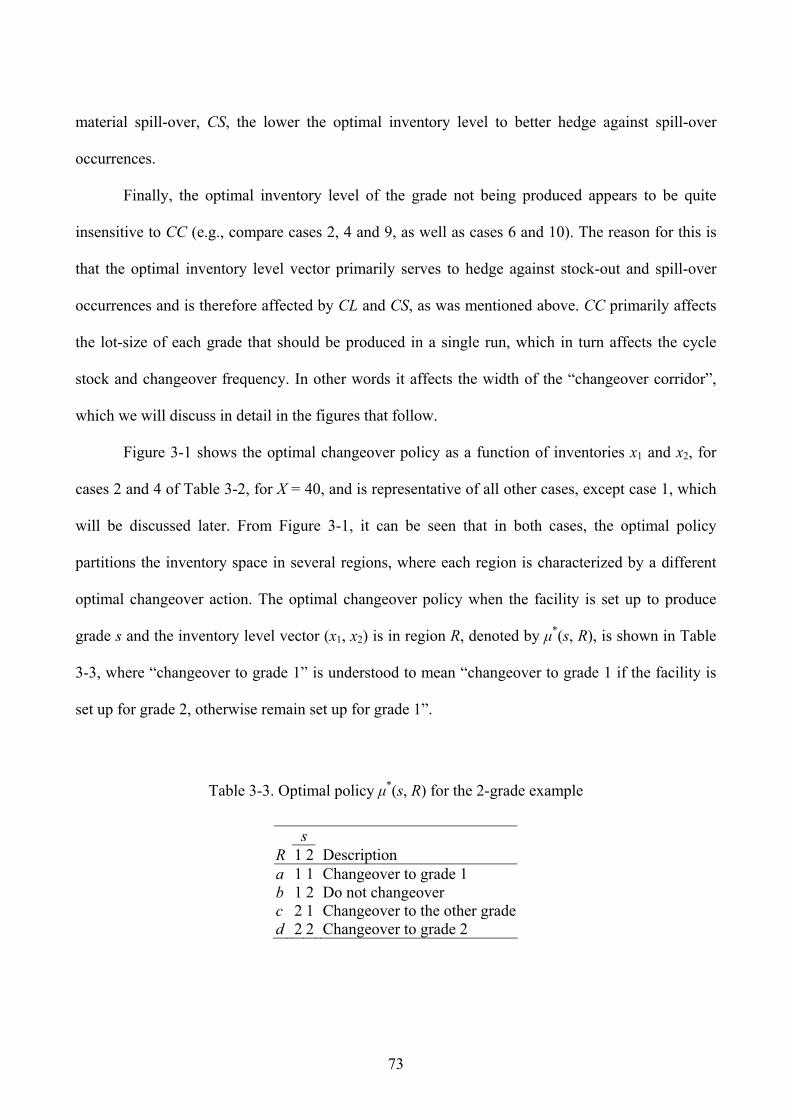
73

material spill-over, CS, the lower the optimal inventory level to better hedge against spill-over

occurrences.

Finally, the optimal inventory level of the grade not being produced appears to be quite

insensitive to CC (e.g., compare cases 2, 4 and 9, as well as cases 6 and 10). The reason for this is

that the optimal inventory level vector primarily serves to hedge against stock-out and spill-over

occurrences and is therefore affected by CL and CS, as was mentioned above. CC primarily affects

the lot-size of each grade that should be produced in a single run, which in turn affects the cycle

stock and changeover frequency. In other words it affects the width of the “changeover corridor”,

which we will discuss in detail in the figures that follow.

Figure 3-1 shows the optimal changeover policy as a function of inventories x1 and x2, for

cases 2 and 4 of Table 3-2, for X = 40, and is representative of all other cases, except case 1, which

will be discussed later. From Figure 3-1, it can be seen that in both cases, the optimal policy

partitions the inventory space in several regions, where each region is characterized by a different

optimal changeover action. The optimal changeover policy when the facility is set up to produce

grade s and the inventory level vector (x1, x2) is in region R, denoted by μ*(s, R), is shown in Table

3-3, where “changeover to grade 1” is understood to mean “changeover to grade 1 if the facility is

set up for grade 2, otherwise remain set up for grade 1”.

Table 3-3. Optimal policy μ*(s, R) for the 2-grade example

s R 1 2 Description a 1 1 Changeover to grade 1 b 1 2 Do not changeover c 2 1 Changeover to the other graded 2 2 Changeover to grade 2

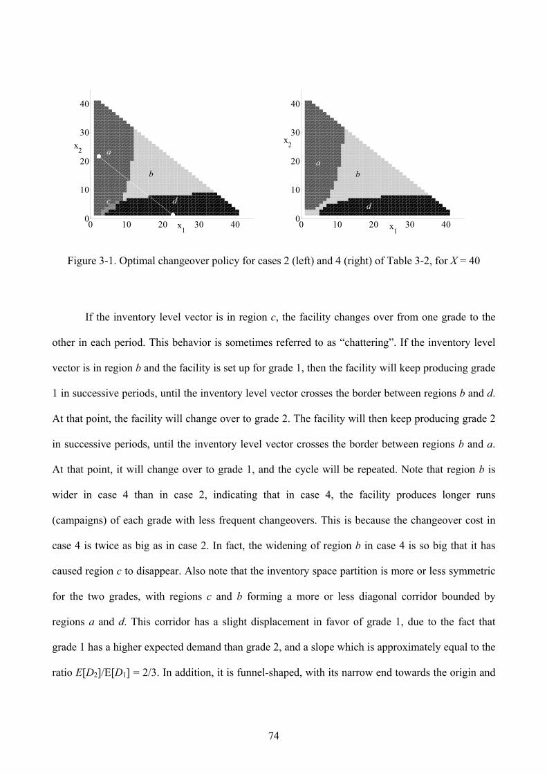
74

0 10 20 30 400

10

20

30

40

x1

x2

b

c d

a

0 10 20 30 400

10

20

30

40

x1

x2

ba

d

Figure 3-1. Optimal changeover policy for cases 2 (left) and 4 (right) of Table 3-2, for X = 40

If the inventory level vector is in region c, the facility changes over from one grade to the

other in each period. This behavior is sometimes referred to as “chattering”. If the inventory level

vector is in region b and the facility is set up for grade 1, then the facility will keep producing grade

1 in successive periods, until the inventory level vector crosses the border between regions b and d.

At that point, the facility will change over to grade 2. The facility will then keep producing grade 2

in successive periods, until the inventory level vector crosses the border between regions b and a.

At that point, it will change over to grade 1, and the cycle will be repeated. Note that region b is

wider in case 4 than in case 2, indicating that in case 4, the facility produces longer runs

(campaigns) of each grade with less frequent changeovers. This is because the changeover cost in

case 4 is twice as big as in case 2. In fact, the widening of region b in case 4 is so big that it has

caused region c to disappear. Also note that the inventory space partition is more or less symmetric

for the two grades, with regions c and b forming a more or less diagonal corridor bounded by

regions a and d. This corridor has a slight displacement in favor of grade 1, due to the fact that

grade 1 has a higher expected demand than grade 2, and a slope which is approximately equal to the

ratio E[D2]/E[D1] = 2/3. In addition, it is funnel-shaped, with its narrow end towards the origin and

75

its wide end towards the inventory state space outer facet, indicating that more frequent

changeovers take place when the inventory levels of both grades are low and the risk of a stock-out

is high, and less frequent changeovers take place when the inventory levels are high. The borders of

the corridor towards its wider end tend to align themselves to the orthogonal lines x1 = c1 and x2 =

c2, respectively, where c1 and c2 are some constants. This means that when the facility is set up for

grade 2, it should change over to grade 1, if x1 drops below c1, irrespectively of x2, as long as x2 is

high. Thus, the optimal changeover policy, which is generally “global” in that changeover decisions

depend on both x1 and x2, becomes “local” in one grade when the inventory level of the other grade

is high.

Note that when s = 1, x1 increases by 2 units and x2 decreases by 2 units per period on

average, while when s = 2, x1 decreases by 3 units and x2 increases by 3 units per period on average.

This implies that on average, the inventory level vector tracks the line x1 + x2 = X′, for some X′ < X.

This line is parallel to the outer facet of the inventory state space, x1 + x2 = X. Under the optimal

changeover policy, the line x1 + x2 = X′ should connect the optimal target inventory level points

(x1*(1), x2

*(1)) and (x1*(2), x2

*(2)). This means that X′ should satisfy: x1*(1) + x2

*(1) = X′ and x1*(2)

+ x2*(2) = X′. Indeed, in all cases shown in Table 3-2, there exists a value of X′ that satisfies the

above two equations. For example, in case 2, X = 40, x1*(1) + x2

*(1) = 1 + 21, x1*(2) + x2

*(2) = 22 +

0, and therefore, X′ = 22, suggesting that under the optimal changeover policy, the FG inventory

buffer should be kept a little over half full. The line connecting the optimal target inventory levels

of the two setup states for this case is shown as a dotted line in Figure 3-1 (left). Under the optimal

changeover policy, the inventory level vector on average moves back and forth along the segment

of that dotted line that falls in region b, as the facility changes over from one grade to the other,

whenever the inventory level vector enters region a or d. Such a trajectory is on average parallel to

the optimal inventory level trajectory of the deterministic version of the problem (where the demand

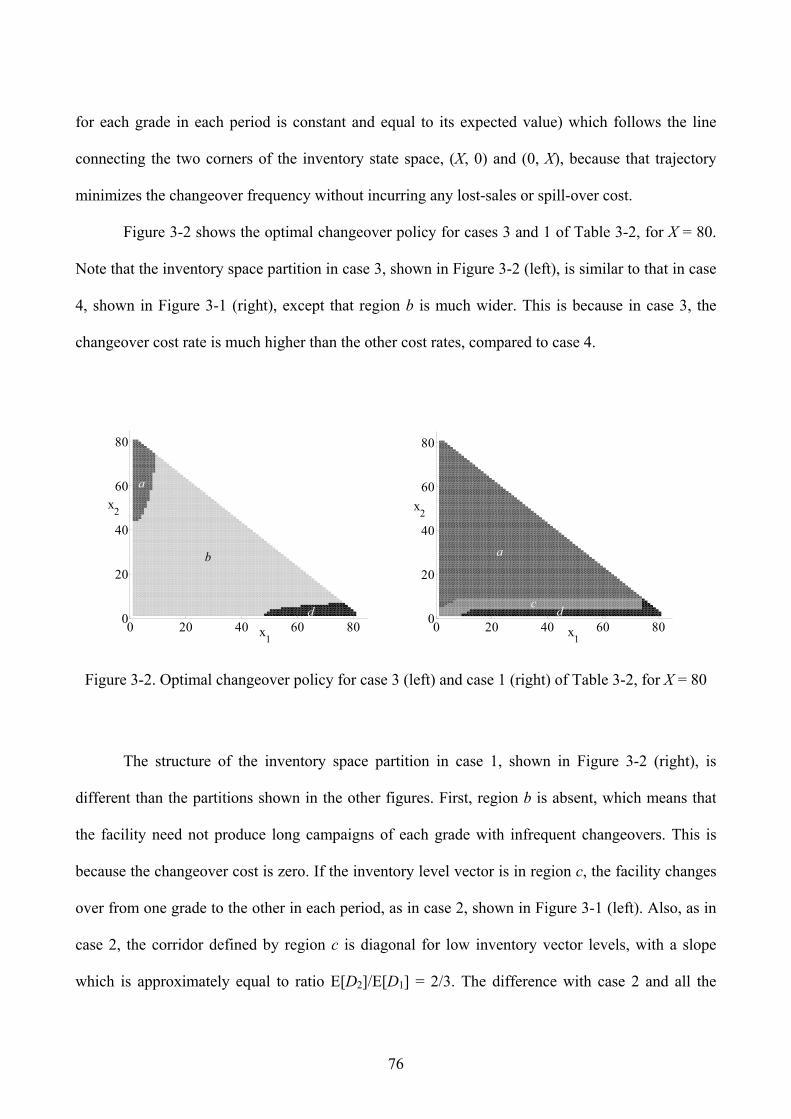
76

for each grade in each period is constant and equal to its expected value) which follows the line

connecting the two corners of the inventory state space, (X, 0) and (0, X), because that trajectory

minimizes the changeover frequency without incurring any lost-sales or spill-over cost.

Figure 3-2 shows the optimal changeover policy for cases 3 and 1 of Table 3-2, for X = 80.

Note that the inventory space partition in case 3, shown in Figure 3-2 (left), is similar to that in case

4, shown in Figure 3-1 (right), except that region b is much wider. This is because in case 3, the

changeover cost rate is much higher than the other cost rates, compared to case 4.

0 20 40 60 800

20

40

60

80

x1

x2

d

a

b

0 20 40 60 800

20

40

60

80

x1

x2

a

dc

Figure 3-2. Optimal changeover policy for case 3 (left) and case 1 (right) of Table 3-2, for X = 80

The structure of the inventory space partition in case 1, shown in Figure 3-2 (right), is

different than the partitions shown in the other figures. First, region b is absent, which means that

the facility need not produce long campaigns of each grade with infrequent changeovers. This is

because the changeover cost is zero. If the inventory level vector is in region c, the facility changes

over from one grade to the other in each period, as in case 2, shown in Figure 3-1 (left). Also, as in

case 2, the corridor defined by region c is diagonal for low inventory vector levels, with a slope

which is approximately equal to ratio E[D2]/E[D1] = 2/3. The difference with case 2 and all the

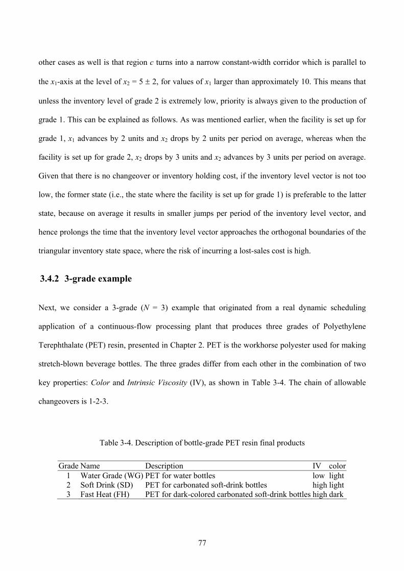
77

other cases as well is that region c turns into a narrow constant-width corridor which is parallel to

the x1-axis at the level of x2 = 5 ± 2, for values of x1 larger than approximately 10. This means that

unless the inventory level of grade 2 is extremely low, priority is always given to the production of

grade 1. This can be explained as follows. As was mentioned earlier, when the facility is set up for

grade 1, x1 advances by 2 units and x2 drops by 2 units per period on average, whereas when the

facility is set up for grade 2, x2 drops by 3 units and x2 advances by 3 units per period on average.

Given that there is no changeover or inventory holding cost, if the inventory level vector is not too

low, the former state (i.e., the state where the facility is set up for grade 1) is preferable to the latter

state, because on average it results in smaller jumps per period of the inventory level vector, and

hence prolongs the time that the inventory level vector approaches the orthogonal boundaries of the

triangular inventory state space, where the risk of incurring a lost-sales cost is high.

3.4.2 3-grade example

Next, we consider a 3-grade (N = 3) example that originated from a real dynamic scheduling

application of a continuous-flow processing plant that produces three grades of Polyethylene

Terephthalate (PET) resin, presented in Chapter 2. PET is the workhorse polyester used for making

stretch-blown beverage bottles. The three grades differ from each other in the combination of two

key properties: Color and Intrinsic Viscosity (IV), as shown in Table 3-4. The chain of allowable

changeovers is 1-2-3.

Table 3-4. Description of bottle-grade PET resin final products

Grade Name Description IV color1 Water Grade (WG) PET for water bottles low light2 Soft Drink (SD) PET for carbonated soft-drink bottles high light3 Fast Heat (FH) PET for dark-colored carbonated soft-drink bottles high dark

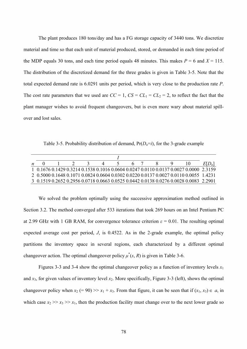
78

The plant produces 180 tons/day and has a FG storage capacity of 3440 tons. We discretize

material and time so that each unit of material produced, stored, or demanded in each time period of

the MDP equals 30 tons, and each time period equals 48 minutes. This makes P = 6 and X = 115.

The distribution of the discretized demand for the three grades is given in Table 3-5. Note that the

total expected demand rate is 6.0291 units per period, which is very close to the production rate P.

The cost rate parameters that we used are CC = 1, CS = CL1 = CL2 = 2, to reflect the fact that the

plant manager wishes to avoid frequent changeovers, but is even more wary about material spill-

over and lost sales.

Table 3-5. Probability distribution of demand, Pr(Dn=i), for the 3-grade example

I n 0 1 2 3 4 5 6 7 8 9 10 E[Dn]1 0.1676 0.1429 0.3214 0.1538 0.1016 0.0604 0.0247 0.0110 0.0137 0.0027 0.0000 2.31592 0.5000 0.1648 0.1071 0.0824 0.0604 0.0302 0.0220 0.0137 0.0027 0.0110 0.0055 1.42313 0.1519 0.2652 0.2956 0.0718 0.0663 0.0525 0.0442 0.0138 0.0276 0.0028 0.0083 2.2901

We solved the problem optimally using the successive approximation method outlined in

Section 3.2. The method converged after 533 iterations that took 269 hours on an Intel Pentium PC

at 2.99 GHz with 1 GB RAM, for convergence tolerance criterion ε = 0.01. The resulting optimal

expected average cost per period, J, is 0.4522. As in the 2-grade example, the optimal policy

partitions the inventory space in several regions, each characterized by a different optimal

changeover action. The optimal changeover policy μ*(s, R) is given in Table 3-6.

Figures 3-3 and 3-4 show the optimal changeover policy as a function of inventory levels x1

and x3, for given values of inventory level x2. More specifically, Figure 3-3 (left), shows the optimal

changeover policy when x2 (= 90) >> x1 + x3. From that figure, it can be seen that if (x1, x3) ∈ a, in

which case x2 >> x3 >> x1, then the production facility must change over to the next lower grade so

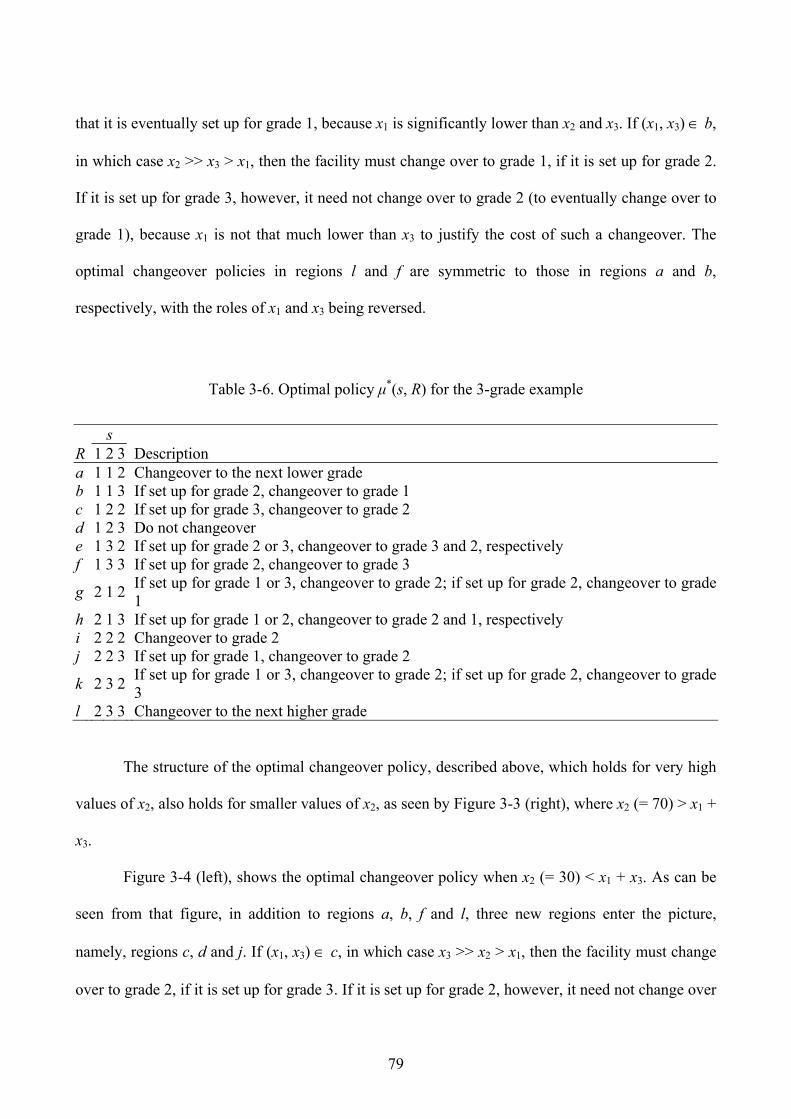
79

that it is eventually set up for grade 1, because x1 is significantly lower than x2 and x3. If (x1, x3) ∈ b,

in which case x2 >> x3 > x1, then the facility must change over to grade 1, if it is set up for grade 2.

If it is set up for grade 3, however, it need not change over to grade 2 (to eventually change over to

grade 1), because x1 is not that much lower than x3 to justify the cost of such a changeover. The

optimal changeover policies in regions l and f are symmetric to those in regions a and b,

respectively, with the roles of x1 and x3 being reversed.

Table 3-6. Optimal policy μ*(s, R) for the 3-grade example

s R 1 2 3 Description a 1 1 2 Changeover to the next lower grade b 1 1 3 If set up for grade 2, changeover to grade 1 c 1 2 2 If set up for grade 3, changeover to grade 2 d 1 2 3 Do not changeover e 1 3 2 If set up for grade 2 or 3, changeover to grade 3 and 2, respectively f 1 3 3 If set up for grade 2, changeover to grade 3

g 2 1 2 If set up for grade 1 or 3, changeover to grade 2; if set up for grade 2, changeover to grade 1

h 2 1 3 If set up for grade 1 or 2, changeover to grade 2 and 1, respectively i 2 2 2 Changeover to grade 2 j 2 2 3 If set up for grade 1, changeover to grade 2

k 2 3 2 If set up for grade 1 or 3, changeover to grade 2; if set up for grade 2, changeover to grade 3

l 2 3 3 Changeover to the next higher grade

The structure of the optimal changeover policy, described above, which holds for very high

values of x2, also holds for smaller values of x2, as seen by Figure 3-3 (right), where x2 (= 70) > x1 +

x3.

Figure 3-4 (left), shows the optimal changeover policy when x2 (= 30) < x1 + x3. As can be

seen from that figure, in addition to regions a, b, f and l, three new regions enter the picture,

namely, regions c, d and j. If (x1, x3) ∈ c, in which case x3 >> x2 > x1, then the facility must change

over to grade 2, if it is set up for grade 3. If it is set up for grade 2, however, it need not change over

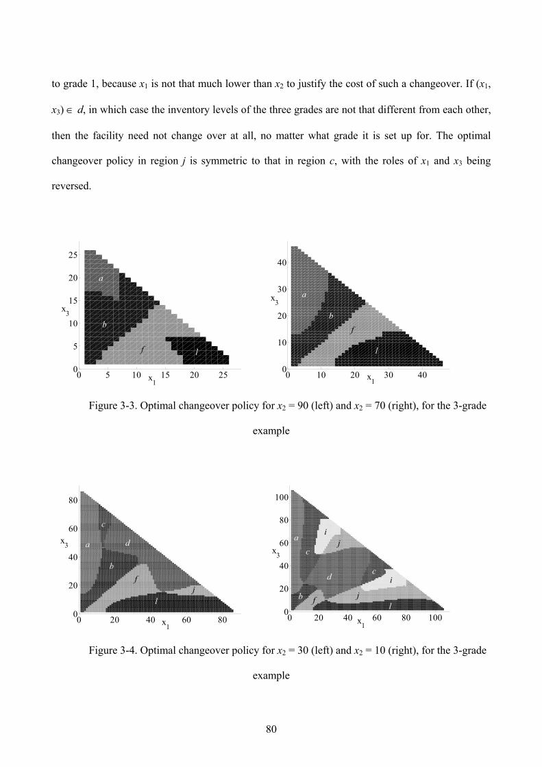
80

to grade 1, because x1 is not that much lower than x2 to justify the cost of such a changeover. If (x1,

x3) ∈ d, in which case the inventory levels of the three grades are not that different from each other,

then the facility need not change over at all, no matter what grade it is set up for. The optimal

changeover policy in region j is symmetric to that in region c, with the roles of x1 and x3 being

reversed.

0 5 10 15 20 250

5

10

15

20

25

x1

x3b

lf

a

0 10 20 30 400

10

20

30

40

x1

x3

l

fb

a

Figure 3-3. Optimal changeover policy for x2 = 90 (left) and x2 = 70 (right), for the 3-grade

example

0 20 40 60 800

20

40

60

80

x1

x3 a

c

d

jl

fb

0 20 40 60 80 1000

20

40

60

80

100

x1

x3

ac

d c

lf

ij

j

i

b

Figure 3-4. Optimal changeover policy for x2 = 30 (left) and x2 = 10 (right), for the 3-grade

example

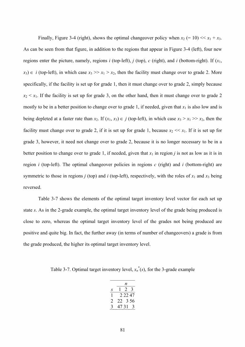
81

Finally, Figure 3-4 (right), shows the optimal changeover policy when x2 (= 10) << x1 + x3.

As can be seen from that figure, in addition to the regions that appear in Figure 3-4 (left), four new

regions enter the picture, namely, regions i (top-left), j (top), c (right), and i (bottom-right). If (x1,

x3) ∈ i (top-left), in which case x3 >> x1 > x2, then the facility must change over to grade 2. More

specifically, if the facility is set up for grade 1, then it must change over to grade 2, simply because

x2 < x1. If the facility is set up for grade 3, on the other hand, then it must change over to grade 2

mostly to be in a better position to change over to grade 1, if needed, given that x1 is also low and is

being depleted at a faster rate than x2. If (x1, x3) ∈ j (top-left), in which case x3 > x1 >> x2, then the

facility must change over to grade 2, if it is set up for grade 1, because x2 << x1. If it is set up for

grade 3, however, it need not change over to grade 2, because it is no longer necessary to be in a

better position to change over to grade 1, if needed, given that x1 in region j is not as low as it is in

region i (top-left). The optimal changeover policies in regions c (right) and i (bottom-right) are

symmetric to those in regions j (top) and i (top-left), respectively, with the roles of x1 and x3 being

reversed.

Table 3-7 shows the elements of the optimal target inventory level vector for each set up

state s. As in the 2-grade example, the optimal target inventory level of the grade being produced is

close to zero, whereas the optimal target inventory level of the grades not being produced are

positive and quite big. In fact, the further away (in terms of number of changeovers) a grade is from

the grade produced, the higher its optimal target inventory level.

Table 3-7. Optimal target inventory level, xn*(s), for the 3-grade example

n s 1 2 31 2 22 472 22 3 563 47 31 3

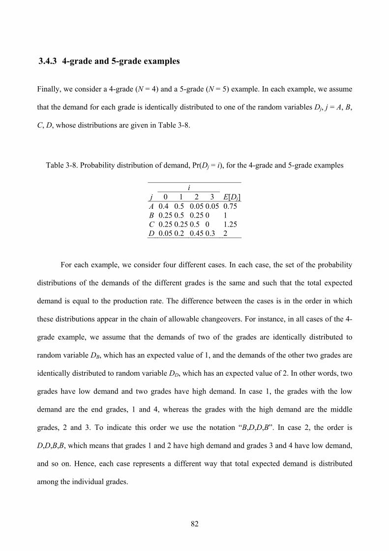
82

3.4.3 4-grade and 5-grade examples

Finally, we consider a 4-grade (N = 4) and a 5-grade (N = 5) example. In each example, we assume

that the demand for each grade is identically distributed to one of the random variables Dj, j = A, B,

C, D, whose distributions are given in Table 3-8.

Table 3-8. Probability distribution of demand, Pr(Dj = i), for the 4-grade and 5-grade examples

i j 0 1 2 3 E[Dj]A 0.4 0.5 0.05 0.05 0.75 B 0.25 0.5 0.25 0 1 C 0.25 0.25 0.5 0 1.25 D 0.05 0.2 0.45 0.3 2

For each example, we consider four different cases. In each case, the set of the probability

distributions of the demands of the different grades is the same and such that the total expected

demand is equal to the production rate. The difference between the cases is in the order in which

these distributions appear in the chain of allowable changeovers. For instance, in all cases of the 4-

grade example, we assume that the demands of two of the grades are identically distributed to

random variable DB, which has an expected value of 1, and the demands of the other two grades are

identically distributed to random variable DD, which has an expected value of 2. In other words, two

grades have low demand and two grades have high demand. In case 1, the grades with the low

demand are the end grades, 1 and 4, whereas the grades with the high demand are the middle

grades, 2 and 3. To indicate this order we use the notation “B,D,D,B”. In case 2, the order is

D,D,B,B, which means that grades 1 and 2 have high demand and grades 3 and 4 have low demand,

and so on. Hence, each case represents a different way that total expected demand is distributed

among the individual grades.

83

First, we solved each case optimally using the successive approximation procedure

described in Section 3.2, for convergence tolerance criterion ε = 0.001. Then, we solved each case

using the heuristic procedure described in Section 3.3. In the implementation of the heuristic

procedure we employed the faster alternative to approximate the sum of the expected lost sales of

the individual grades, described at the end of Section 3.3, which uses expression (3.5) to estimate

the aggregate inventory levels of the composite grades, for values of α ranging from 0 to 1 with a

step size of 0.1. In all cases, we assumed that CC = CS = CLn = 1, n = 1, …, 5, and P = 6.

The results for the 4-grade example, for X = 30, are shown in Table 3-9. The CPU times

reported are in hours on an Intel Core i7 PC at 2.67 GHz with 3 GB RAM. For the heuristic, we

show the total CPU time in hours that it took to solve the (N – 2) 3-grade sub-problems and

generate the heuristic policy, but not the time it took to evaluate the heuristic policy. As was

mentioned at the end of Section 3.3, the time it takes to evaluate the heuristic policy using the value

iteration method is significant, whereas the alternative of using discrete-time system simulation is

much faster. In all cases of the 4-grade problem, we used the value iteration method. The optimal

value of α in the heuristic procedure is denoted by α*, and the corresponding expected average cost

per period is denoted by Jh(α*). The last column of Table 3-9 shows the percent cost increase

between the heuristic and the optimal policy. The complete set of the results of the heuristic policy

evaluated both with the value iteration method and simulation, for different values of α, are shown

in Appendix E.

In case 1, the grades with the highest expected demands are in the middle of the chain of

allowable changeovers, whereas in case 4, they are at the two ends of the chain. Hence, case 1

represents a situation where the dispersion of the total expected demand among the individual

grades is relatively low, because most of the time the production facility will be changing over

between the highly demanded grades, 2 and 3, which are adjacent. Case 4, on the other hand,

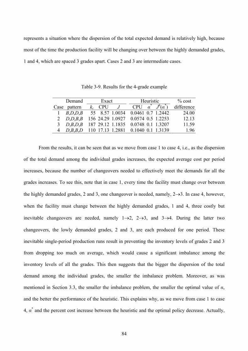
84

represents a situation where the dispersion of the total expected demand is relatively high, because

most of the time the production facility will be changing over between the highly demanded grades,

1 and 4, which are spaced 3 grades apart. Cases 2 and 3 are intermediate cases.

Table 3-9. Results for the 4-grade example

Demand Exact Heuristic % cost Case pattern kc CPU J CPU α* Jh(α*) difference

1 B,D,D,B 55 8.57 1.0034 0.0461 0.7 1.2442 24.00 2 D,D,B,B 156 24.29 1.0927 0.0574 0.5 1.2253 12.13 3 D,B,D,B 187 29.12 1.1835 0.0748 0.1 1.3207 11.59 4 D,B,B,D 110 17.13 1.2881 0.1040 0.1 1.3139 1.96

From the results, it can be seen that as we move from case 1 to case 4, i.e., as the dispersion

of the total demand among the individual grades increases, the expected average cost per period

increases, because the number of changeovers needed to effectively meet the demands for all the

grades increases. To see this, note that in case 1, every time the facility must change over between

the highly demanded grades, 2 and 3, one changeover is needed, namely, 2→3. In case 4, however,

when the facility must change between the highly demanded grades, 1 and 4, three costly but

inevitable changeovers are needed, namely 1→2, 2→3, and 3→4. During the latter two

changeovers, the lowly demanded grades, 2 and 3, are each produced for one period. These

inevitable single-period production runs result in preventing the inventory levels of grades 2 and 3

from dropping too much on average, which would cause a significant imbalance among the

inventory levels of all the grades. This then suggests that the bigger the dispersion of the total

demand among the individual grades, the smaller the imbalance problem. Moreover, as was

mentioned in Section 3.3, the smaller the imbalance problem, the smaller the optimal value of α,

and the better the performance of the heuristic. This explains why, as we move from case 1 to case

4, α* and the percent cost increase between the heuristic and the optimal policy decrease. Actually,

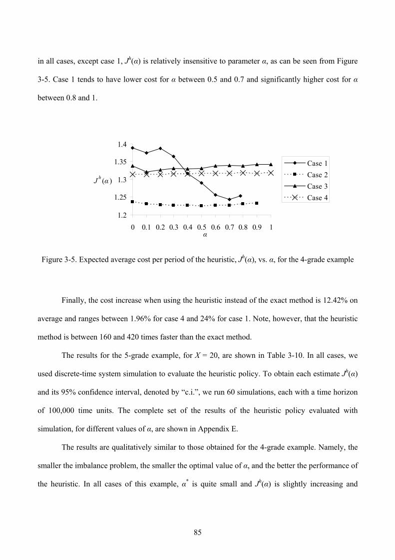
85

in all cases, except case 1, Jh(α) is relatively insensitive to parameter α, as can be seen from Figure

3-5. Case 1 tends to have lower cost for α between 0.5 and 0.7 and significantly higher cost for α

between 0.8 and 1.

1.2

1.25

1.3

1.35

1.4

0 0.1 0.2 0.3 0.4 0.5 0.6 0.7 0.8 0.9 1

J h (α )

Case 1Case 2Case 3Case 4

α

Figure 3-5. Expected average cost per period of the heuristic, Jh(α), vs. α, for the 4-grade example

Finally, the cost increase when using the heuristic instead of the exact method is 12.42% on

average and ranges between 1.96% for case 4 and 24% for case 1. Note, however, that the heuristic

method is between 160 and 420 times faster than the exact method.

The results for the 5-grade example, for X = 20, are shown in Table 3-10. In all cases, we

used discrete-time system simulation to evaluate the heuristic policy. To obtain each estimate Jh(α)

and its 95% confidence interval, denoted by “c.i.”, we run 60 simulations, each with a time horizon

of 100,000 time units. The complete set of the results of the heuristic policy evaluated with

simulation, for different values of α, are shown in Appendix E.

The results are qualitatively similar to those obtained for the 4-grade example. Namely, the

smaller the imbalance problem, the smaller the optimal value of α, and the better the performance of

the heuristic. In all cases of this example, α* is quite small and Jh(α) is slightly increasing and

86

relatively insensitive to parameter α, at least for values of α smaller that 0.5, as can be seen from

Figure 3-6. The cost increase when using the heuristic instead of the exact method ranges between

7.59% for case 4 and 14.46% for case 1 and is 12.75% on average, which is practically the same as

the average cost difference in the 4-grade example. The heuristic method, however, is between 600

and 1700 times faster than the exact method, which is quite significant.

Table 3-10. Results for the 5-grade example

Demand Exact Heuristic % cost Case pattern kc CPU J CPU α* Jh(α*) (95% c.i.) increase

1 A,C,D,C,A 35 38.05 2.6520 0.0223v 0.1 3.0355 ± 0.0016 14.46 2 D,C,C,A,A 71 78.70 3.0016 0.1293v 0.1 3.4512 ± 0.0015 14.98 3 D,C,A,A,C 129 141.21 3.4916 0.1761v 0 3.8759 ± 0.0020 11.00 4 D,A,C,A,C 129 140.39 3.6572 0.1758v 0 3.9348 ± 0.0020 7.59

2.003.004.005.006.007.008.009.00

10.0011.00

0 0.1 0.2 0.3 0.4 0.5 0.6 0.7 0.8 0.9 1

J h (α )

Case 1Case 2Case 3Case 4

α

Figure 3-6. Expected average cost per period of the heuristic, Jh(α), vs. α, for the 5-grade example

3.5 Conclusions

We studied a new version of the SELSP, for which we developed a MDP model. For problems with

2 and 3 grades, we numerically solved the MDP problem and obtained useful insight into the

influence of the problem parameters and structure of the optimal changeover policy, which

87

partitions the state space into different regions, each characterized by different optimal changeover

actions.

For problems with N grades, N > 3, we developed a heuristic solution procedure which is

based on approximating the original multi-grade problem by (N – 2) 3-grade sub-problems and

numerically solving each sub-problem. We tested the heuristic for problems with 4 and 5 grades.

For the 4-grade examples, the heuristic procedure was 160-420 times faster than the numerical

procedure for solving the exact problem and the heuristic solution performed on average 12.42%

worse that the exact solution. For the 5-grade examples, the heuristic procedure was 600-1700 times

faster than the numerical procedure for solving the exact problem and the heuristic solution

performed on average 12.75% worse that the exact solution. The fact that the performance of the

heuristic solution is more or less the same for the 4-grade and 5-grade problems is an encouraging

sign for problems with more than 5 grades. The numerical results showed that the bigger the

dispersion of the total expected demand among the individual grades, the better the performance of

the heuristic.

We can easily solve problems with more than 5 grades using the heuristic; however, it is

impossible to compare the performance of the changeover policy that the heuristic generates to that

of the optimal changeover policy, because it is impossible to even start the value iteration method to

find the optimal policy, as the state space grows dramatically with the number of grades and simply

there is not enough computer memory to store it. For example, for a problem with N = 6 and X = 20,

the state space contains (6⋅206)/2 = 192×106 points.

88

89

Chapter 4 Dissertation summary

In Chapter 2, we developed an MILP model for the production scheduling of a multi-grade PET

processing chemical plant. We also presented an application of the model on a real case study,

along with some discussion that provides insight into its behavior. The model minimizes the cost

associated with the number of grade changeovers, while also ensuring that the capacity constraints

of the problem are not violated and that the demand for final products is satisfied on time. The

model incorporates all aspects of the problem under consideration and can be easily extended to

address additional ones that may arise in different situations, because of the large number of

decision variables that enhances its flexibility. We believe that the main contribution of this work is

that it addresses efficiently an important practical application, whose solution exhibits high

complexity.

A number of possible directions for future research arise from this work. Firstly, one could

try to develop a continuous-time model formulation for this problem and compare its results to

those of the discrete-time model that we present here. Our guess is that the development of such a

model would be demanding and would not necessarily be computationally more efficient than the

present discrete-time model. It would, however, represent more accurately the real production and

storage process, which is continuous in nature. A second possible direction would be to relax some

of the hard constraints, e.g. the on-time delivery of demand constraints (2.24), (2.25) and (2.27)

and/or the safety stock constraints (2.21) and (2.29), as was discussed at the end of Section 3, and

90

see if this leads to significant benefits. Another possible direction would be to develop a more

accurate SELSP formulation than the one presented in Chapter 3 to better design the safety stock

levels, or resort to some stochastic integer programming technique to solve the scheduling problem

under uncertainties. A recent work relevant to this subject is due to Sand and Engell (2004), who

utilize two-stage stochastic integer programming techniques to solve scheduling problems of

flexible chemical batch processes that exhibit uncertainties. Finally, one could try to fit the

scheduling model developed in this dissertation within a broader planning and supply chain

framework, e.g., as discussed in Kallrath (2002).

In Chapter 3, we studied a new version of the SELSP, for which we developed a MDP

model. For problems with 2 and 3 grades, we numerically solved the MDP problem and obtained

useful insight into the influence of the problem parameters and structure of the optimal changeover

policy, which partitions the state space into different regions, each characterized by different

optimal changeover actions.

For problems with N grades, N > 3, we developed a heuristic solution procedure which is

based on approximating the original multi-grade problem by (N – 2) 3-grade sub-problems and

numerically solving each sub-problem. We tested the heuristic for problems with 4 and 5 grades.

For the 4-grade examples, the heuristic procedure was 160-420 times faster than the numerical

procedure for solving the exact problem and the heuristic solution performed on average 12.42%

worse that the exact solution. For the 5-grade examples, the heuristic procedure was 600-1700 times

faster than the numerical procedure for solving the exact problem and the heuristic solution

performed on average 12.75% worse that the exact solution. The fact that the performance of the

heuristic solution is more or less the same for the 4-grade and 5-grade problems is an encouraging

sign for problems with more than 5 grades. The numerical results showed that the bigger the

91

dispersion of the total expected demand among the individual grades, the better the performance of

the heuristic.

We can easily solve problems with more than 5 grades using the heuristic; however, it is

impossible to compare the performance of the changeover policy that the heuristic generates to that

of the optimal changeover policy, because it is impossible to even start the value iteration method to

find the optimal policy, as the state space grows dramatically with the number of grades and simply

there is not enough computer memory to store it. For example, for a problem with N = 6 and X = 20,

the state space contains (6⋅206)/2 = 192×106 points.

A possible direction for future research would be to try to develop a better heuristic that

somehow uses the optimal value functions of the sub-problems, although we should point out that

our initial experimentation with this possibility has not been encouraging. Another direction would

be to extend the model so as to accommodate other types of FG storage than the common FG buffer

that we assumed in our model. For example, one could consider multiple parallel FG buffers (e.g.,

industrial silos) that can store only one grade at a time, or two serial FG buffers, e.g., one for storing

bulk FGs and the second for storing packaged FGs, as is the case in the real application described in

Chapter 2.

92

93

Bibliography

Anupindi, R., Tayur, S. 1998. Managing stochastic multiproduct systems: model, measures, and

analysis. Operations Research 46 (3) S98-S111.

Bok, J. and Park, S., (1998). Continuous-time modeling for short-term scheduling of multipurpose

pipeless plants. Industrial and Engineering Chemistry Research 37 (9), 3652-3659.

Bourland, K.E., Yano, C.A. 1994. The strategic use of capacity slack in the economic lot scheduling

problem with random demand. Management Science 40 (12) 1690-1704.

Castro, P.M. and Grossmann, I.E., (2006). An efficient MILP model for short-term scheduling of

single stage batch plants. Computers and Chemical Engineering 30, 1003-1018.

Chase, C., Serrano, J., Ramadge, P.J. 1993. Periodicity and chaos from switched flow systems:

contrasting examples of discretely controlled continuous systems. IEEE Transactions on

Automatic Control 38 (1), 70-83.

Dallery, Y. and Gershwin, S.B. (1992). Manufacturing flow line systems: A review of models and

analytical results. Queueing Systems 12 (1-2), 3-94.

Doganis, P., Sarimveis, H., Bafas, G. and Koufos, D., (2005). An MILP model for optimal

scheduling of the lubricant production plant. Chemical Engineering Communications 192 (8),

1067-1084.

94

Elhafsi, M., Bai, S.X. 1997. Optimal and near-optimal control of a two-part-type stochastic

manufacturing system with dynamic setups. Production and Operations Management 6 (4) 419-

438.

Elmaghraby, S.E. 1978. The economic lot scheduling problem (ELSP): review and extensions.

Management Science 24 (6), 587-598.

Federgruen, A., Katalan, Z. 1996. The stochastic economic lot scheduling problem: cyclical base

stock policies with idle times. Management Science 42 (6) 783-796.

Floudas, C.A. and Lin, X., (2004). Continuous-time versus discrete time approaches for scheduling

of chemical processes: A review. Computers and Chemical Engineering 28 (11), 2109-2129.

Floudas, C.A. and Lin, X., (2005). Mixed integer linear programming in process scheduling:

Modeling, algorithms, and applications. Annals of Operations Research 139 (1), 131-162.

Fourer, R., Gay, D.M. and Kernighan, B.W., (2002). AMPL: A Modeling Language for

Mathematical Programming. Duxbury Press.

Fransoo, J.C., Sridharan, V., Bertrand, J.W.M. 1995. A hierarchical approach for capacity

coordination in multiple products single-machine production systems with stationary stochastic

demands. European Journal of Operational Research 86 (1) 57-72.

Gallego, G. 1990. Scheduling the production of several items with random demands in a single

facility. Management Science 36 (12) 1579-1592.

Gallego, G. 1994. When is a base stock policy optimal in recovering disrupted cyclic schedules?

Naval Research Logistics 41 (1) 317-333.

Giannelos, N.F. and Georgiadis, M.C., (2002). A novel event-driven formulation for short-term

scheduling of multipurpose continuous processes. Industrial and Engineering Chemistry

Research 41 (10), 2431-2439.

95

Graves, S.C. 1980. The multi-product production cycling problem. AIIE Transactions 12 (3), 233-

240.

Grossmann, I.E., Quesada, J., Raman, R. and Voudouris, V., (1996). Mixed integer optimization

techniques for the design and scheduling of batch processes, Batch Processing Systems

Engineering, G. V. Reklaitis, A. K. Sunol, D. W. T. Rippin and O. Hortacsu (eds.), Springer,

Berlin, 451-494.

Grünow, M., Günther, H-O. and Lehman, M. (2002). Campaign planning for multi-stage batch

processes in the chemical industry. OR Spectrum 24 (3), 281-314.

Hui, C., Gupta, A. and van der Meulen, H.A.J., (2000). A novel MILP formulation for short-term

scheduling of multi-stage multi-product batch plants with sequence-dependent constraints.

Computers and Chemical Engineering 24 (12), 2705-2717.

Ierapetritou, M.G. and Floudas, C.A., (1998a). Effective continuous-time formulation for short-term

scheduling. I. Multipurpose batch processes. Industrial and Engineering Chemistry Research 37

(11), 4341-4359.

Ierapetritou M.G. and Floudas, C.A., (1998b). Effective continuous-time formulation for short-term

scheduling. II. Continuous and semicontinuous processes. Industrial and Engineering

Chemistry Research 37 (11), 4360-4374.

Janak, S.L. and Floudas, C.A., (2008). Improving unit-specific event based continuous-time

approaches for batch processes: Integrality gap and task splitting. Computers and Chemical

Engineering 32, 913-955.

Janak, S.L., Lin, X. and Floudas, C.A., (2004). Enhanced continuous-time unit-specific event based

formulation for short-term scheduling of multipurpose batch processes: Resource constraints

and mixed storage policies. Industrial and Engineering Chemistry Research 43 (10), 2516-

2533.

96

Janak, S.L., Floudas, C.A., Kallrath, J. and Vormbrock, N., (2006a). Production scheduling of a

large-scale industrial batch plant. I. Short-term and medium-term scheduling. Industrial and

Engineering Chemistry Research 45 (25), 8234-8252.

Janak, S.L., Floudas, C.A., Kallrath, J. and Vormbrock, N., (2006b). Production scheduling of a

large-scale industrial batch plant. II. Reactive scheduling. Industrial and Engineering Chemistry

Research 45 (25), 8253-8269.

Kallrath, J., (2002). Planning and scheduling in the process industry. OR Spectrum 24 (3), 219-250.

Karmarkar, U.S., Yoo, J. 1994. The stochastic dynamic product cycling problem. European Journal

of Operational Research 73 (2), 360-373.

Kimemia, J.G., Gershwin, S.B. 1983. An algorithm for the computer control of production in

flexible manufacturing systems. IIE Transactions 15 (4), 353-362.

Kondili, E., Pantelides, C.C. and Sargent, R.W.H., (1993). A general algorithm for short-term

scheduling of batch operations. I. MILP formulation. Computers and Chemical Engineering 17

(2), 211-227.

Leachman, R.C., Gascon, A. 1998. A heuristic policy for multi-item, single-machine production

systems with time-varying stochastic demands. Management Science 34 (3) 377-390.

Lee, H.M., Pinto, J.M. and Grossmann, I.E., (1996). Mixed-integer linear programming model for

refinery short-term scheduling of crude oil unloading with inventory management. Industrial

and Engineering Chemistry Research 35 (5), 1630-1641.

Liberopoulos, G., Caramanis, M. 1997. Numerical investigation of optimal policies for production

flow control and set-up scheduling: lessons from two-part-type failure prone FMSs. International

Journal of Production Research 35 (8), 2109-2133.

97

Lin, X. and Floudas, C.A., (2001). Design, synthesis and scheduling of multipurpose batch plants

via an effective continuous-time formulation. Computers and Chemical Engineering 25, 665-

674.

Mahadevan, R., Doyle, F.J.III and Allcock, A.C., (2007). Control-relevant scheduling of polymer

grade transitions. AIChE Journal 48 (8), 1754-1764.

Markowitz, D.M., Reiman, M.I., Wein, L.M. 2000. The stochastic economic lot scheduling

problem: heavy traffic analysis of dynamic cyclic policies. Operations Research 48 (1) 136-154.

Markowitz, D.M., Wein, L.M. 2001. Heavy traffic analysis of dynamic cyclic policies: a unified

treatment of the single machine scheduling problem. Operations Research 49 (2) 246-270.

McGehee, J.F., Johnson, J.A. and Bertelli, C., (2004). Maximizing PET SSP line profitability

through world scale process design and operations. POLYESTER 2004: 9th World Congress, 7-

9 December 2004, Zurich, Switzerland.

Méndez, C.A. and Cerdá, J., (2002). An efficient MILP continuous-time formulation for short-term

scheduling of multiproduct continuous facilities. Computers and Chemical Engineering 26 (4-

5), 687-695.

Méndez, C.A., Cerdá, J., Grossmann, I.E., Harjunkoski, L. and Fahl, M., (2006). State-of-the art

review of optimization methods for short-term scheduling of batch processes. Computers and

Chemical Engineering 30, 913-946.

Mockus, L. and Reklaitis, G.V., (1999). Continuous time representation approach to batch and

continuous process scheduling: 1. MINLP formulation. Industrial and Engineering Chemistry

Research 38 (1), 197-203.

Neumann, K., Schwindt C. and Trautmann, N., (2002). Advanced production scheduling for batch

plants in process industries. OR Spectrum 24 (3), 251-279.

98

Nyström R.H., Franke, R., Harjunkoski, I., and Kroll, A. (2005). Production campaign planning

including grade transition sequencing and dynamic optimization. Computers and Chemical

Engineering 29 (10) 2163-2179.

Pinto, J.M. and Grossmann, I.E., (1995). A continuous time mixed integer linear programming

model for short term scheduling of multistage batch plants. Industrial and Engineering

Chemistry Research 34 (9), 3037-3051.

Pinto, J.M., Turkay, A., Bolio, B. and Grossmann, I.E., (1997). A continuous-time MILP

optimization for short-term scheduling of batch plants. Computers and Chemical Engineering

22 (9), 1297-1308.

Pinto, J.M. and Grossmann, I.E., (1998). Assignment and sequencing models for the scheduling of

process systems. Annals of Operations Research 81, 433-466.

Prata, A., Oldenburg, J., Kroll, A. and Marquardt, W., (2008). Integrated scheduling and dynamic

optimization of grade transitions for a continuous polymerization reactor. Computers and

Chemical Engineering 32 (3), 463-476.

Qiu, M.M. and Burch, E.E. (1997). Hierarchical production planning and scheduling in a multi-

product, multi-machine environment. International Journal of Production Research 35 (11),

3023-3042.

Qiu, J., Loulou, R. 1995. Multiproduct production/inventory control under random demands. IEEE

Transactions on Automatic Control 40 (2), 350-356.

Reklaitis, G.V. (1992). Overview of scheduling and planning of batch process operations. NATO

Advanced Study Institute – Batch Process Systems Engineering, Antalya, Turkey.

Salomon, M. 1991. Deterministic lotsizing models for production planning. Lecture Notes in

Economics and Mathematical Systems. Springer-Verlag, Berlin.

99

Sand, G. and Engell, S. (2004). Modeling and solving real-time scheduling problems by stochastic

integer programming. Computers and Chemical Engineering 28, 1087-1103.

Shaik, M.A. and Floudas, C.A., (2007). Improved unit-specific event-based continuous-time model

for short-term scheduling of continuous processes: Rigorous treatment of storage requirements.

Industrial and Engineering Chemistry Research 46 (6), 1764-1779.

Shaik, M.A., Janak, S.L. and Floudas, C.A., (2006). Continuous-time models for short-term

scheduling of multipurpose batch plants: A comparative study. Industrial and Engineering

Chemistry Research 45 (18), 6190-6209.

Shaik, M.A., Floudas, C.A., Kallrath, J. and Pitz, H.J., (2009). Production scheduling of a large-

scale industrial continuous plant: Short-term and medium-term scheduling. Computers and

Chemical Engineering 33 (3), 670-686.

Sharifnia, A., Caramanis, M., Gershwin, S.B. 1991. Dynamic setup scheduling and flow control in

manufacturing systems. Discrete Event Dynamic Systems 1 (2) 149-175.

Sox, C.R., Jackson, P.L., Bowman, A., Muckstadt, J.A. 1999. A review of the stochastic lot

scheduling problem. International Journal of Production Economics 62 (3), 181-200.

Sox, C.R., Muckstadt, J.A. 1997. Optimization-based planning for the stochastic lot-sizing problem.

IIE Transactions 29 (5), 349-357.

Suerie, C. (2005). Time continuity in discrete time models: New approaches for production

planning in process industries. Lectures Notes in Economics and Mathematical Systems, 552,

Springer, Berlin, Germany.

Terrazas-Moreno, S., Flores-Tlacuahuac, A. and Grossmann, I.E., (2007). Simultaneous cyclic

scheduling and optimal control of polymerizations reactors. AIChE Journal 53 (9), 2301-2315.

Tousain, R.L. and Bosgra, O.H., (2006). Market-oriented scheduling and economic optimization of

continuous multi-grade chemical processes. Journal of Process Control 16 (3), 291 – 302.

100

Vergin, R.C., Lee, T.N. 1978. Scheduling rules for the multiple product single-machine system with

stochastic demand. INFOR 16 (1), 64-73.

Wang, K., Lohl, T., Stobbe, M. and Engell, S., (2000). A genetic algorithm for online-scheduling of

a multiproduct polymer batch plant. Computers and Chemical Engineering 24, 393-400.

Winands, E.M.M., Adan, I.J.B.F., van Houtum, G.J. 2005. The stochastic economic lot scheduling

problem: a survey. Working paper. Beta Research School for Operations Management and

Logistics, Technical University of Eindhoven.

Zipkin, P.H. 1986. Models for design and control of stochastic multi-item batch production

systems. Operations Research 34 (1) 91-104.

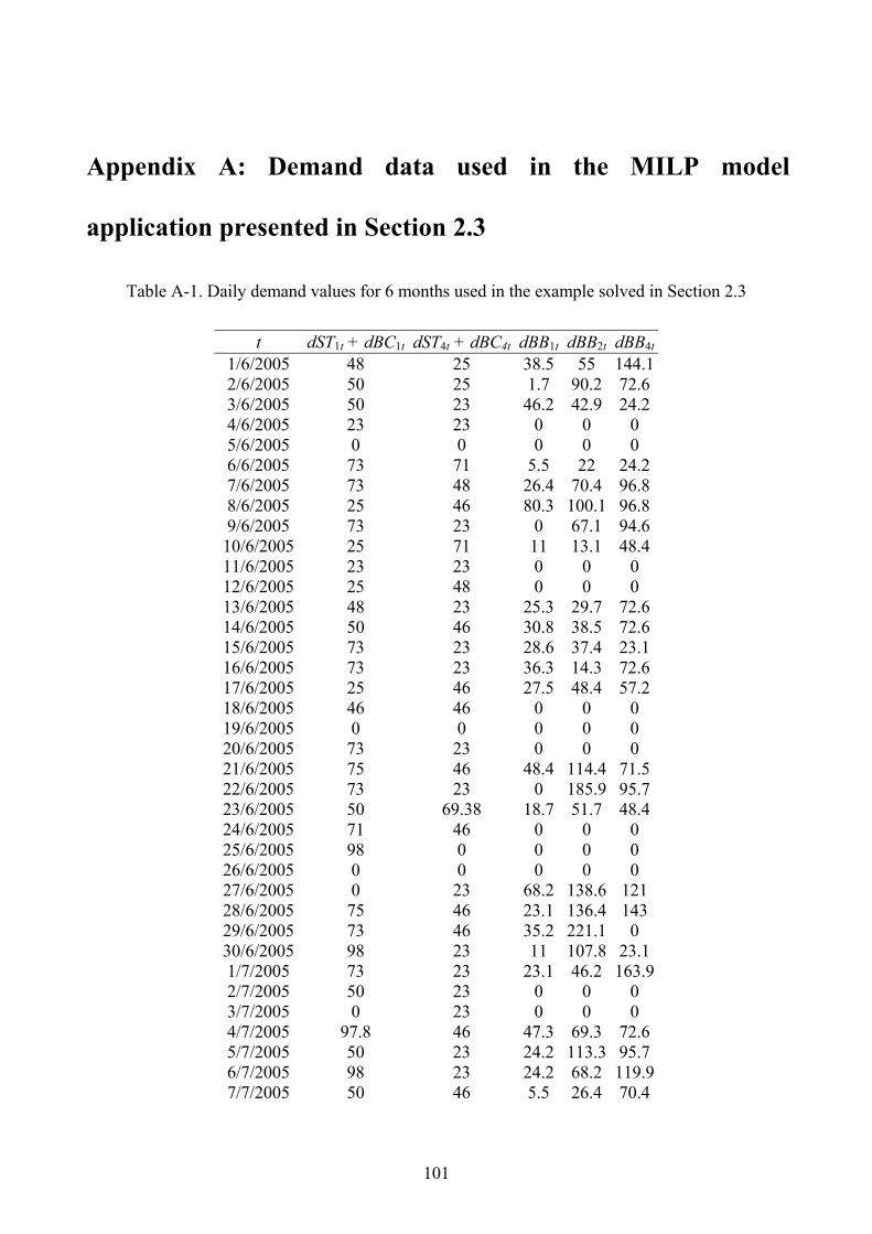
101

Appendix A: Demand data used in the MILP model

application presented in Section 2.3

Table A-1. Daily demand values for 6 months used in the example solved in Section 2.3

t dST1t + dBC1t dST4t + dBC4t dBB1t dBB2t dBB4t 1/6/2005 48 25 38.5 55 144.1 2/6/2005 50 25 1.7 90.2 72.6 3/6/2005 50 23 46.2 42.9 24.2 4/6/2005 23 23 0 0 0 5/6/2005 0 0 0 0 0 6/6/2005 73 71 5.5 22 24.2 7/6/2005 73 48 26.4 70.4 96.8 8/6/2005 25 46 80.3 100.1 96.8 9/6/2005 73 23 0 67.1 94.6 10/6/2005 25 71 11 13.1 48.4 11/6/2005 23 23 0 0 0 12/6/2005 25 48 0 0 0 13/6/2005 48 23 25.3 29.7 72.6 14/6/2005 50 46 30.8 38.5 72.6 15/6/2005 73 23 28.6 37.4 23.1 16/6/2005 73 23 36.3 14.3 72.6 17/6/2005 25 46 27.5 48.4 57.2 18/6/2005 46 46 0 0 0 19/6/2005 0 0 0 0 0 20/6/2005 73 23 0 0 0 21/6/2005 75 46 48.4 114.4 71.5 22/6/2005 73 23 0 185.9 95.7 23/6/2005 50 69.38 18.7 51.7 48.4 24/6/2005 71 46 0 0 0 25/6/2005 98 0 0 0 0 26/6/2005 0 0 0 0 0 27/6/2005 0 23 68.2 138.6 121 28/6/2005 75 46 23.1 136.4 143 29/6/2005 73 46 35.2 221.1 0 30/6/2005 98 23 11 107.8 23.1 1/7/2005 73 23 23.1 46.2 163.9 2/7/2005 50 23 0 0 0 3/7/2005 0 23 0 0 0 4/7/2005 97.8 46 47.3 69.3 72.6 5/7/2005 50 23 24.2 113.3 95.7 6/7/2005 98 23 24.2 68.2 119.9 7/7/2005 50 46 5.5 26.4 70.4

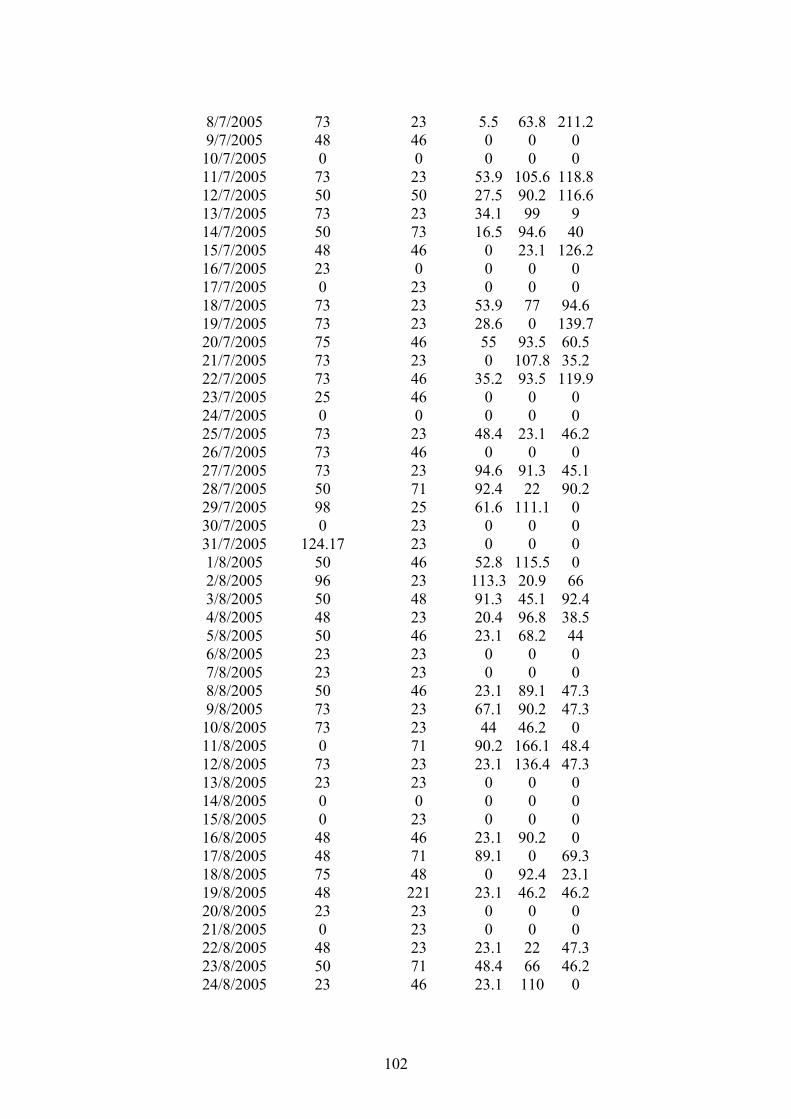
102

8/7/2005 73 23 5.5 63.8 211.2 9/7/2005 48 46 0 0 0 10/7/2005 0 0 0 0 0 11/7/2005 73 23 53.9 105.6 118.8 12/7/2005 50 50 27.5 90.2 116.6 13/7/2005 73 23 34.1 99 9 14/7/2005 50 73 16.5 94.6 40 15/7/2005 48 46 0 23.1 126.2 16/7/2005 23 0 0 0 0 17/7/2005 0 23 0 0 0 18/7/2005 73 23 53.9 77 94.6 19/7/2005 73 23 28.6 0 139.7 20/7/2005 75 46 55 93.5 60.5 21/7/2005 73 23 0 107.8 35.2 22/7/2005 73 46 35.2 93.5 119.9 23/7/2005 25 46 0 0 0 24/7/2005 0 0 0 0 0 25/7/2005 73 23 48.4 23.1 46.2 26/7/2005 73 46 0 0 0 27/7/2005 73 23 94.6 91.3 45.1 28/7/2005 50 71 92.4 22 90.2 29/7/2005 98 25 61.6 111.1 0 30/7/2005 0 23 0 0 0 31/7/2005 124.17 23 0 0 0 1/8/2005 50 46 52.8 115.5 0 2/8/2005 96 23 113.3 20.9 66 3/8/2005 50 48 91.3 45.1 92.4 4/8/2005 48 23 20.4 96.8 38.5 5/8/2005 50 46 23.1 68.2 44 6/8/2005 23 23 0 0 0 7/8/2005 23 23 0 0 0 8/8/2005 50 46 23.1 89.1 47.3 9/8/2005 73 23 67.1 90.2 47.3 10/8/2005 73 23 44 46.2 0 11/8/2005 0 71 90.2 166.1 48.4 12/8/2005 73 23 23.1 136.4 47.3 13/8/2005 23 23 0 0 0 14/8/2005 0 0 0 0 0 15/8/2005 0 23 0 0 0 16/8/2005 48 46 23.1 90.2 0 17/8/2005 48 71 89.1 0 69.3 18/8/2005 75 48 0 92.4 23.1 19/8/2005 48 221 23.1 46.2 46.2 20/8/2005 23 23 0 0 0 21/8/2005 0 23 0 0 0 22/8/2005 48 23 23.1 22 47.3 23/8/2005 50 71 48.4 66 46.2 24/8/2005 23 46 23.1 110 0

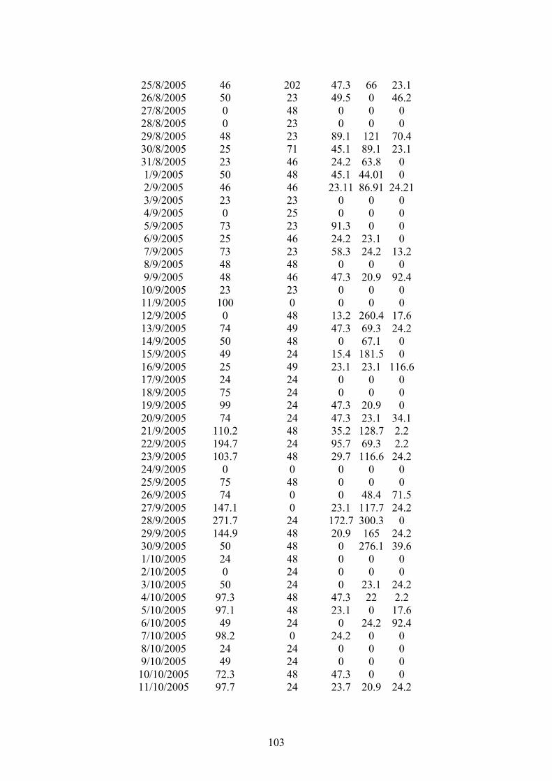
103

25/8/2005 46 202 47.3 66 23.1 26/8/2005 50 23 49.5 0 46.2 27/8/2005 0 48 0 0 0 28/8/2005 0 23 0 0 0 29/8/2005 48 23 89.1 121 70.4 30/8/2005 25 71 45.1 89.1 23.1 31/8/2005 23 46 24.2 63.8 0 1/9/2005 50 48 45.1 44.01 0 2/9/2005 46 46 23.11 86.91 24.21 3/9/2005 23 23 0 0 0 4/9/2005 0 25 0 0 0 5/9/2005 73 23 91.3 0 0 6/9/2005 25 46 24.2 23.1 0 7/9/2005 73 23 58.3 24.2 13.2 8/9/2005 48 48 0 0 0 9/9/2005 48 46 47.3 20.9 92.4 10/9/2005 23 23 0 0 0 11/9/2005 100 0 0 0 0 12/9/2005 0 48 13.2 260.4 17.6 13/9/2005 74 49 47.3 69.3 24.2 14/9/2005 50 48 0 67.1 0 15/9/2005 49 24 15.4 181.5 0 16/9/2005 25 49 23.1 23.1 116.6 17/9/2005 24 24 0 0 0 18/9/2005 75 24 0 0 0 19/9/2005 99 24 47.3 20.9 0 20/9/2005 74 24 47.3 23.1 34.1 21/9/2005 110.2 48 35.2 128.7 2.2 22/9/2005 194.7 24 95.7 69.3 2.2 23/9/2005 103.7 48 29.7 116.6 24.2 24/9/2005 0 0 0 0 0 25/9/2005 75 48 0 0 0 26/9/2005 74 0 0 48.4 71.5 27/9/2005 147.1 0 23.1 117.7 24.2 28/9/2005 271.7 24 172.7 300.3 0 29/9/2005 144.9 48 20.9 165 24.2 30/9/2005 50 48 0 276.1 39.6 1/10/2005 24 48 0 0 0 2/10/2005 0 24 0 0 0 3/10/2005 50 24 0 23.1 24.2 4/10/2005 97.3 48 47.3 22 2.2 5/10/2005 97.1 48 23.1 0 17.6 6/10/2005 49 24 0 24.2 92.4 7/10/2005 98.2 0 24.2 0 0 8/10/2005 24 24 0 0 0 9/10/2005 49 24 0 0 0 10/10/2005 72.3 48 47.3 0 0 11/10/2005 97.7 24 23.7 20.9 24.2

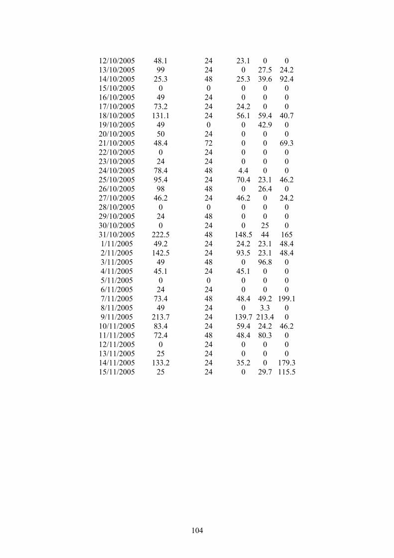
104

12/10/2005 48.1 24 23.1 0 0 13/10/2005 99 24 0 27.5 24.2 14/10/2005 25.3 48 25.3 39.6 92.4 15/10/2005 0 0 0 0 0 16/10/2005 49 24 0 0 0 17/10/2005 73.2 24 24.2 0 0 18/10/2005 131.1 24 56.1 59.4 40.7 19/10/2005 49 0 0 42.9 0 20/10/2005 50 24 0 0 0 21/10/2005 48.4 72 0 0 69.3 22/10/2005 0 24 0 0 0 23/10/2005 24 24 0 0 0 24/10/2005 78.4 48 4.4 0 0 25/10/2005 95.4 24 70.4 23.1 46.2 26/10/2005 98 48 0 26.4 0 27/10/2005 46.2 24 46.2 0 24.2 28/10/2005 0 0 0 0 0 29/10/2005 24 48 0 0 0 30/10/2005 0 24 0 25 0 31/10/2005 222.5 48 148.5 44 165 1/11/2005 49.2 24 24.2 23.1 48.4 2/11/2005 142.5 24 93.5 23.1 48.4 3/11/2005 49 48 0 96.8 0 4/11/2005 45.1 24 45.1 0 0 5/11/2005 0 0 0 0 0 6/11/2005 24 24 0 0 0 7/11/2005 73.4 48 48.4 49.2 199.1 8/11/2005 49 24 0 3.3 0 9/11/2005 213.7 24 139.7 213.4 0 10/11/2005 83.4 24 59.4 24.2 46.2 11/11/2005 72.4 48 48.4 80.3 0 12/11/2005 0 24 0 0 0 13/11/2005 25 24 0 0 0 14/11/2005 133.2 24 35.2 0 179.3 15/11/2005 25 24 0 29.7 115.5

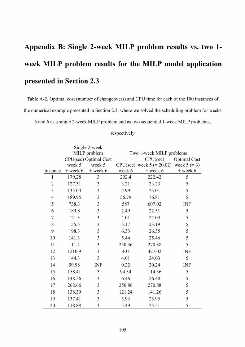
105

Appendix B: Single 2-week MILP problem results vs. two 1-

week MILP problem results for the MILP model application

presented in Section 2.3

Table A-2. Optimal cost (number of changeovers) and CPU time for each of the 100 instances of

the numerical example presented in Section 2.3, where we solved the scheduling problem for weeks

5 and 6 as a single 2-week MILP problem and as two sequential 1-week MILP problems,

respectively

Single 2-week

MILP problem Two 1-week MILP problems

Instance

CPU(sec) week 5

+ week 6

Optimal Costweek 5

+ week 6 CPU(sec)

week 6

CPU(sec) week 5 (= 20.02)

+ week 6

Optimal Cost week 5 (= 3)

+ week 6 1 179.28 3 202.4 222.42 5 2 127.31 3 3.21 23.23 5 3 135.04 3 2.99 23.01 5 4 189.95 3 56.79 76.81 5 5 738.3 3 587 607.02 INF 6 189.8 3 2.49 22.51 5 7 121.3 3 4.01 24.03 5 8 155.5 3 3.17 23.19 5 9 198.3 3 6.33 26.35 5 10 141.3 3 5.44 25.46 5 11 111.4 3 250.36 270.38 5 12 1210.9 3 407 427.02 INF 13 144.3 3 4.01 24.03 5 14 99.98 INF 0.22 20.24 INF 15 158.41 3 94.34 114.36 5 16 148.56 3 6.46 26.48 5 17 268.66 3 250.86 270.88 5 18 138.39 3 121.24 141.26 5 19 137.41 3 5.93 25.95 5 20 118.88 3 5.49 25.51 5

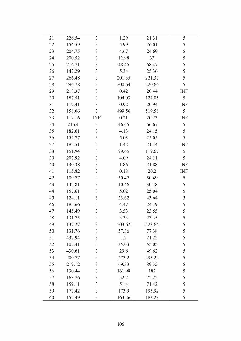
106

21 226.54 3 1.29 21.31 5 22 156.59 3 5.99 26.01 5 23 204.75 3 4.67 24.69 5 24 200.52 3 12.98 33 5 25 216.71 3 48.45 68.47 5 26 142.29 3 5.34 25.36 5 27 266.48 3 201.35 221.37 5 28 296.78 3 200.64 220.66 5 29 218.37 3 0.42 20.44 INF 30 187.51 3 104.03 124.05 5 31 119.41 3 0.92 20.94 INF 32 158.06 3 499.56 519.58 5 33 112.16 INF 0.21 20.23 INF 34 216.4 3 46.65 66.67 5 35 182.61 3 4.13 24.15 5 36 152.77 3 5.03 25.05 5 37 183.51 3 1.42 21.44 INF 38 151.94 3 99.65 119.67 5 39 207.92 3 4.09 24.11 5 40 130.38 3 1.86 21.88 INF 41 115.82 3 0.18 20.2 INF 42 109.77 3 30.47 50.49 5 43 142.81 3 10.46 30.48 5 44 157.61 3 5.02 25.04 5 45 124.11 3 23.62 43.64 5 46 183.66 3 4.47 24.49 5 47 145.49 3 3.53 23.55 5 48 131.75 3 3.33 23.35 5 49 137.27 3 503.62 523.64 5 50 131.76 3 57.36 77.38 5 51 437.94 3 1.2 21.22 5 52 102.41 3 35.03 55.05 5 53 430.61 3 29.6 49.62 5 54 200.77 3 273.2 293.22 5 55 219.12 3 69.33 89.35 5 56 130.44 3 161.98 182 5 57 163.76 3 52.2 72.22 5 58 159.11 3 51.4 71.42 5 59 177.42 3 173.9 193.92 5 60 152.49 3 163.26 183.28 5

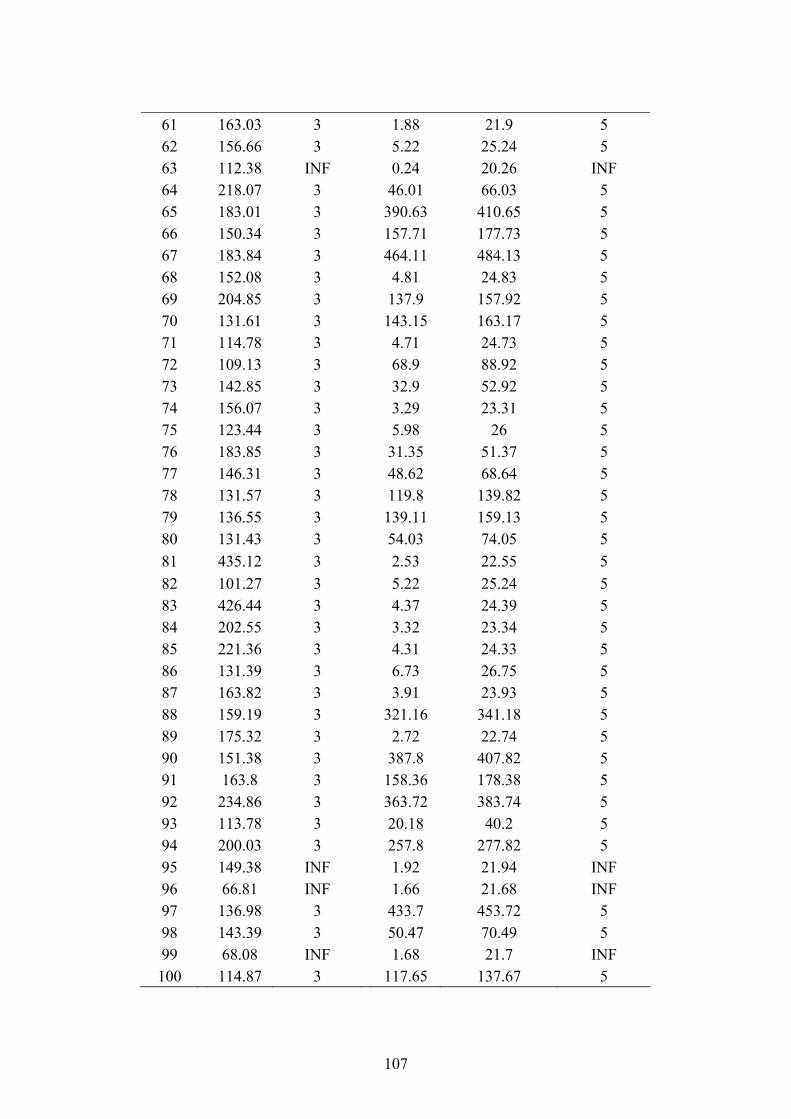
107

61 163.03 3 1.88 21.9 5 62 156.66 3 5.22 25.24 5 63 112.38 INF 0.24 20.26 INF 64 218.07 3 46.01 66.03 5 65 183.01 3 390.63 410.65 5 66 150.34 3 157.71 177.73 5 67 183.84 3 464.11 484.13 5 68 152.08 3 4.81 24.83 5 69 204.85 3 137.9 157.92 5 70 131.61 3 143.15 163.17 5 71 114.78 3 4.71 24.73 5 72 109.13 3 68.9 88.92 5 73 142.85 3 32.9 52.92 5 74 156.07 3 3.29 23.31 5 75 123.44 3 5.98 26 5 76 183.85 3 31.35 51.37 5 77 146.31 3 48.62 68.64 5 78 131.57 3 119.8 139.82 5 79 136.55 3 139.11 159.13 5 80 131.43 3 54.03 74.05 5 81 435.12 3 2.53 22.55 5 82 101.27 3 5.22 25.24 5 83 426.44 3 4.37 24.39 5 84 202.55 3 3.32 23.34 5 85 221.36 3 4.31 24.33 5 86 131.39 3 6.73 26.75 5 87 163.82 3 3.91 23.93 5 88 159.19 3 321.16 341.18 5 89 175.32 3 2.72 22.74 5 90 151.38 3 387.8 407.82 5 91 163.8 3 158.36 178.38 5 92 234.86 3 363.72 383.74 5 93 113.78 3 20.18 40.2 5 94 200.03 3 257.8 277.82 5 95 149.38 INF 1.92 21.94 INF 96 66.81 INF 1.66 21.68 INF 97 136.98 3 433.7 453.72 5 98 143.39 3 50.47 70.49 5 99 68.08 INF 1.68 21.7 INF 100 114.87 3 117.65 137.67 5

108

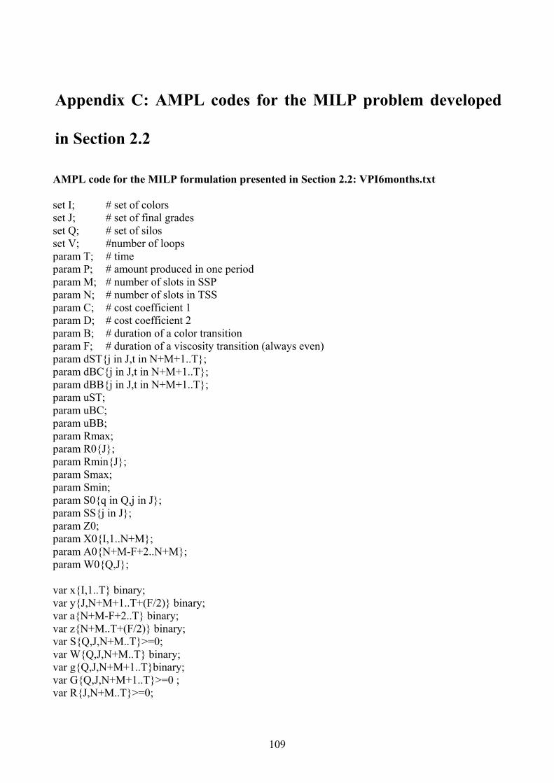
109

Appendix C: AMPL codes for the MILP problem developed

in Section 2.2

AMPL code for the MILP formulation presented in Section 2.2: VPI6months.txt set I; # set of colors set J; # set of final grades set Q; # set of silos set V; #number of loops param T; # time param P; # amount produced in one period param M; # number of slots in SSP param N; # number of slots in TSS param C; # cost coefficient 1 param D; # cost coefficient 2 param B; # duration of a color transition param F; # duration of a viscosity transition (always even) param dSTj in J,t in N+M+1..T; param dBCj in J,t in N+M+1..T; param dBBj in J,t in N+M+1..T; param uST; param uBC; param uBB; param Rmax; param R0J; param RminJ; param Smax; param Smin; param S0q in Q,j in J; param SSj in J; param Z0; param X0I,1..N+M; param A0N+M-F+2..N+M; param W0Q,J; var xI,1..T binary; var yJ,N+M+1..T+(F/2) binary; var aN+M-F+2..T binary; var zN+M..T+(F/2) binary; var SQ,J,N+M..T>=0; var WQ,J,N+M..T binary; var gQ,J,N+M+1..Tbinary; var GQ,J,N+M+1..T>=0 ; var RJ,N+M..T>=0;

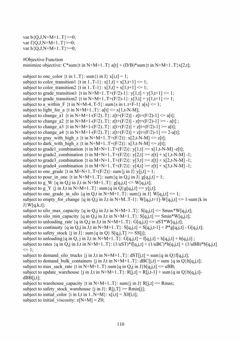
110

var bQ,J,N+M+1..T>=0; var fQ,J,N+M+1..T>=0; var hQ,J,N+M+1..T>=0; #Objective Function minimize objective: C*sumt in N+M+1..T a[t] + (D/B)*sumt in N+M+1..Tx[2,t]; subject to one_color t in 1..T: sumi in I x[i,t] = 1; subject to color_transition1 t in 1..T-1: x[1,t] + x[3,t+1] <= 1; subject to color_transition2 t in 1..T-1: x[3,t] + x[1,t+1] <= 1; subject to grade_transition1 t in N+M+1..T+(F/2)-1: y[1,t] + y[3,t+1] <= 1; subject to grade_transition2 t in N+M+1..T+(F/2)-1: y[3,t] + y[1,t+1] <= 1; subject to a_within_F t in N+M-4..T-5: sums in t..t+F-1 a[s] <= 1; subject to light_for_a t in N+M+1..T: a[t] <= x[1,t-N-M]; subject to change_a1 t in N+M+1-(F/2)..T: z[t+(F/2)] - z[t+(F/2)-1] <= a[t]; subject to change_a2 t in N+M+1-(F/2)..T: z[t+(F/2)] - z[t+(F/2)-1] >= - a[t] ; subject to change_a3 t in N+M+1-(F/2)..T: z[t+(F/2)] + z[t+(F/2)-1] >= a[t]; subject to change_a4 t in N+M+1-(F/2)..T: z[t+(F/2)] + z[t+(F/2)-1] <= 2-a[t]; subject to gray_with_high_z t in N+M+1..T+(F/2): x[2,t-N-M] <= z[t]; subject to dark_with_high_z t in N+M+1..T+(F/2): x[3,t-N-M] <= z[t]; subject to grade1_combination t in M+N+1..T+(F/2): y[1,t] >= x[1,t-N-M] -z[t]; subject to grade2_combination t in M+N+1..T+(F/2): y[2,t] >= z[t] + x[1,t-N-M] -1; subject to grade3_combination t in M+N+1..T+(F/2): y[3,t] >= z[t] + x[2,t-N-M] -1; subject to grade4_combination t in M+N+1..T+(F/2): y[4,t] >= z[t] + x[3,t-N-M] -1; subject to one_grade t in M+N+1..T+(F/2): sumj in J y[j,t] = 1; subject to pour_in_one t in N+M+1..T: sumq in Q,j in J g[q,j,t] = 1; subject to g_W q in Q,j in J,t in N+M+1..T: g[q,j,t] <= W[q,j,t]; subject to g_Y j in J,t in N+M+1..T: sumq in Qg[q,j,t] <= y[j,t]; subject to one_grade_in_silo q in Q,t in N+M+1..T: sumj in J W[q,j,t] <= 1; subject to empty_for_change q in Q,j in J,t in N+M..T-1: W[q,j,t+1]-W[q,j,t] <= 1-sumk in JW[q,k,t]; subject to silo_max_capacity q in Q,j in J,t in N+M+1..T: S[q,j,t] <= Smax*W[q,j,t]; subject to silo_min_capacity q in Q,j in J,t in N+M+1..T: S[q,j,t] >= Smin*W[q,j,t]; subject to unloading_rate q in Q,j in J,t in N+M+1..T: G[q,j,t] <= uST*W[q,j,t]; subject to continuity q in Q,j in J,t in N+M+1..T: S[q,j,t] = S[q,j,t-1] + P*g[q,j,t] - G[q,j,t]; subject to safety_stock j in J: sumq in Q S[q,j,T] >= SS[j]; subject to unloadingq in Q, j in J,t in N+M+1..T: G[q,j,t] = f[q,j,t] + h[q,j,t] + b[q,j,t] ; subject to rates q in Q,j in J,t in N+M+1..T: (1/uST)*f[q,j,t] + (1/uBC)*h[q,j,t] + (1/uBB)*b[q,j,t] <= 1; subject to demand_silo_trucks j in J,t in N+M+1..T: dST[j,t] = sumq in Qf[q,j,t]; subject to demand_bulk_containers j in J,t in N+M+1..T: dBC[j,t] = sum q in Qh[q,j,t]; subject to max_sack_rate t in N+M+1..T:sumq in Q,j in Jb[q,j,t] <= uBB; subject to update_warehouse j in J,t in N+M+1..T: R[j,t] = R[j,t-1] + sumq in Qb[q,j,t]-dBB[j,t]; subject to warehouse_capacity t in N+M+1..T: sumj in J R[j,t] <= Rmax; subject to safety_stock_warehouse j in J: R[j,T] >= Rmin[j]; subject to initial_color i in I,t in 1..N+M: x[i,t] = X0[i,t]; subject to initial_viscosity: z[N+M] = Z0;

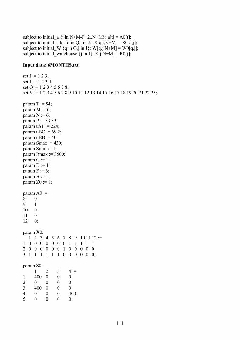
111

subject to initial_a t in N+M-F+2..N+M: a[t] = A0[t]; subject to initial_silo q in Q,j in J: S[q,j,N+M] = S0[q,j]; subject to initial_W q in Q,j in J: W[q,j,N+M] = W0[q,j]; subject to initial_warehouse j in J: R[j,N+M] = R0[j]; Input data: 6MONTHS.txt set I := 1 2 3; set J := 1 2 3 4; set Q := 1 2 3 4 5 6 7 8; set V := 1 2 3 4 5 6 7 8 9 10 11 12 13 14 15 16 17 18 19 20 21 22 23; param T := 54; param M := 6; param N := 6; param P := 33.33; param uST := 224; param uBC := 69.2; param uBB := 40; param Smax := 430; param Smin := 1; param Rmax := 3500; param C := 1; param D := 1; param F := 6; param B := 1; param Z0 := 1; param A0 := 8 0 9 1 10 0 11 0 12 0; param X0: 1 2 3 4 5 6 7 8 9 10 11 12 := 1 0 0 0 0 0 0 0 1 1 1 1 1 2 0 0 0 0 0 0 1 0 0 0 0 0 3 1 1 1 1 1 1 0 0 0 0 0 0; param S0: 1 2 3 4 := 1 400 0 0 0 2 0 0 0 0 3 400 0 0 0 4 0 0 0 400 5 0 0 0 0

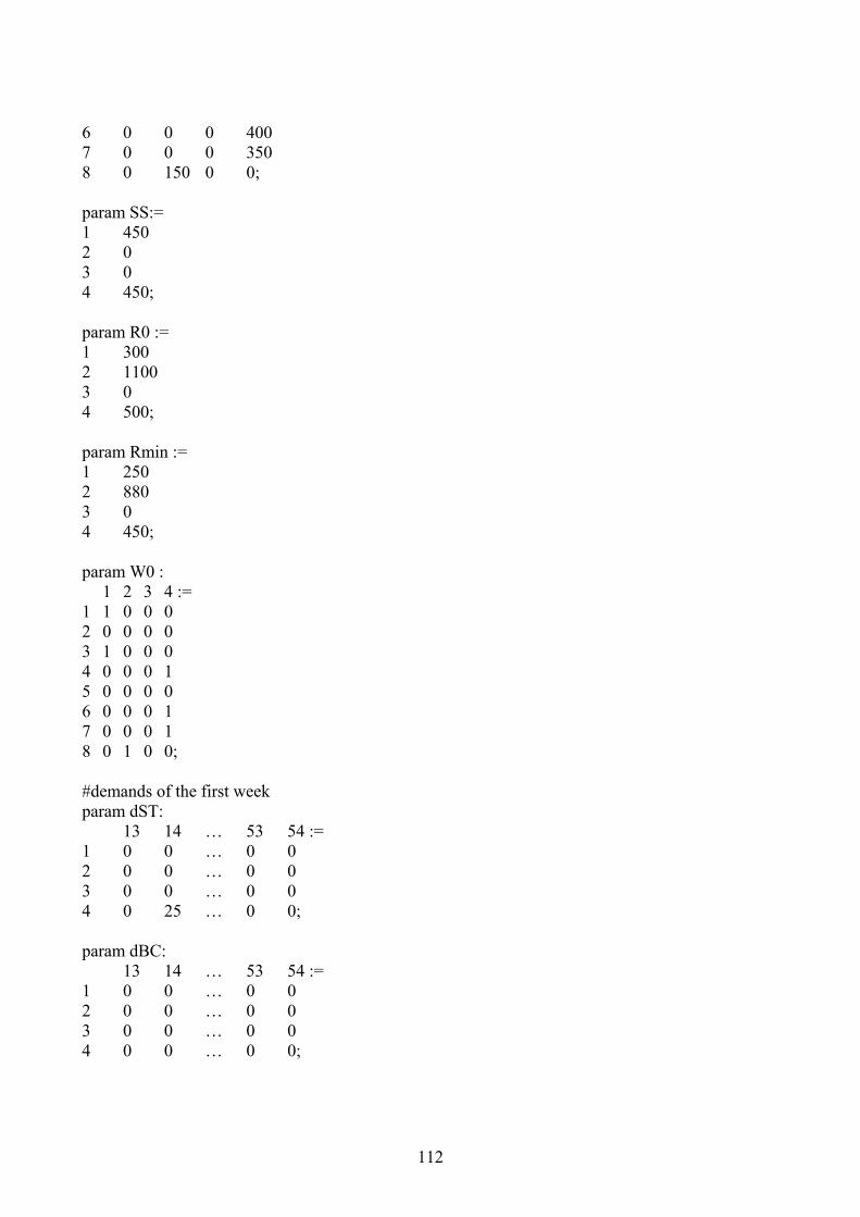
112

6 0 0 0 400 7 0 0 0 350 8 0 150 0 0; param SS:= 1 450 2 0 3 0 4 450; param R0 := 1 300 2 1100 3 0 4 500; param Rmin := 1 250 2 880 3 0 4 450; param W0 : 1 2 3 4 := 1 1 0 0 0 2 0 0 0 0 3 1 0 0 0 4 0 0 0 1 5 0 0 0 0 6 0 0 0 1 7 0 0 0 1 8 0 1 0 0; #demands of the first week param dST: 13 14 … 53 54 := 1 0 0 … 0 0 2 0 0 … 0 0 3 0 0 … 0 0 4 0 25 … 0 0; param dBC: 13 14 … 53 54 := 1 0 0 … 0 0 2 0 0 … 0 0 3 0 0 … 0 0 4 0 0 … 0 0;

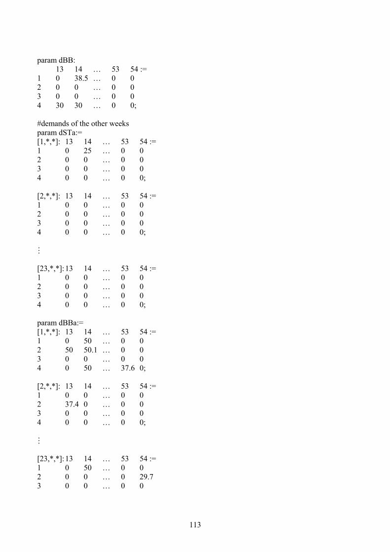
113

param dBB: 13 14 … 53 54 := 1 0 38.5 … 0 0 2 0 0 … 0 0 3 0 0 … 0 0 4 30 30 … 0 0; #demands of the other weeks param dSTa:= [1,*,*]: 13 14 … 53 54 := 1 0 25 … 0 0 2 0 0 … 0 0 3 0 0 … 0 0 4 0 0 … 0 0; [2,*,*]: 13 14 … 53 54 := 1 0 0 … 0 0 2 0 0 … 0 0 3 0 0 … 0 0 4 0 0 … 0 0;

[23,*,*]: 13 14 … 53 54 := 1 0 0 … 0 0 2 0 0 … 0 0 3 0 0 … 0 0 4 0 0 … 0 0; param dBBa:= [1,*,*]: 13 14 … 53 54 := 1 0 50 … 0 0 2 50 50.1 … 0 0 3 0 0 … 0 0 4 0 50 … 37.6 0; [2,*,*]: 13 14 … 53 54 := 1 0 0 … 0 0 2 37.4 0 … 0 0 3 0 0 … 0 0 4 0 0 … 0 0;

[23,*,*]: 13 14 … 53 54 := 1 0 50 … 0 0 2 0 0 … 0 29.7 3 0 0 … 0 0

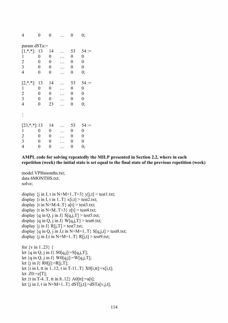
114

4 0 0 … 0 0; param dSTa:= [1,*,*]: 13 14 … 53 54 := 1 0 0 … 0 0 2 0 0 … 0 0 3 0 0 … 0 0 4 0 0 … 0 0; [2,*,*]: 13 14 … 53 54 := 1 0 0 … 0 0 2 0 0 … 0 0 3 0 0 … 0 0 4 0 23 … 0 0;

[23,*,*]: 13 14 … 53 54 := 1 0 0 … 0 0 2 0 0 … 0 0 3 0 0 … 0 0 4 0 0 … 0 0; AMPL code for solving repeatedly the MILP presented in Section 2.2, where in each repetition (week) the initial state is set equal to the final state of the previous repetition (week) model VPI6months.txt; data 6MONTHS.txt; solve; display j in J, t in N+M+1..T+3 y[j,t] > test1.txt; display i in I, t in 1..T x[i,t] > test2.txt; display t in N+M-4..T a[t] > test3.txt; display t in N+M..T+3 z[t] > test4.txt; display q in Q, j in J S[q,j,T] > test5.txt; display q in Q, j in J W[q,j,T] > test6.txt; display j in J R[j,T] > test7.txt; display q in Q, j in J,t in N+M+1..T S[q,j,t] > test8.txt; display j in J,t in N+M+1..T R[j,t] > test9.txt; for v in 1..23 let q in Q, j in J S0[q,j]:=S[q,j,T]; let q in Q, j in J W0[q,j]:=W[q,j,T]; let j in J R0[j]:=R[j,T]; let i in I, tt in 1..12, t in T-11..T X0[i,tt]:=x[i,t]; let Z0:=z[T]; let t in T-4..T, tt in 8..12 A0[tt]:=a[t]; let j in J, t in N+M+1..T dST[j,t]:=dSTa[v,j,t];

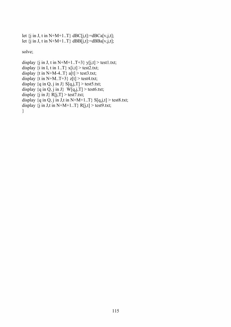
115

let j in J, t in N+M+1..T dBC[j,t]:=dBCa[v,j,t]; let j in J, t in N+M+1..T dBB[j,t]:=dBBa[v,j,t]; solve; display j in J, t in N+M+1..T+3 y[j,t] > test1.txt; display i in I, t in 1..T x[i,t] > test2.txt; display t in N+M-4..T a[t] > test3.txt; display t in N+M..T+3 z[t] > test4.txt; display q in Q, j in J S[q,j,T] > test5.txt; display q in Q, j in J W[q,j,T] > test6.txt; display j in J R[j,T] > test7.txt; display q in Q, j in J,t in N+M+1..T S[q,j,t] > test8.txt; display j in J,t in N+M+1..T R[j,t] > test9.txt;

116

117

Appendix D: Matlab codes for implementing the exact and

heuristic solution procedures developed in Sections 3.2 and 3.3

In this appendix, we present the programming codes (in Matlab) for implementing the exact and

heuristic solution procedures for problems with 4 and 5 grades. We also give the codes that we used

to obtain the 2D graphs showing the optimal changeover presented in Section 2.3.

Codes for 4-grade problems Program DP_4D_EXACT Program that solves the SELSP problem for 4 grades using the exact solution procedure

Input N = number of grades X = FGI storage capacity PMAX = production rate CC = changeover cost CS = spillover cost LS(1) = lost sales cost for grade 1 LS(2) = lost sales cost for grade 2 e = small positive number DD = table of demand values for grades 1-4 PP = table of probabilities of demands for grades 1-4 DIM = dimension of tables DD and PP n1 = special setup state BIG = vey large number X11 = special inventory level of grade 1 X21 = special inventory level of grade 2 X31 = special inventory level of grade 3 X41 = special inventory level of grade 4 Output U(n,x1,x2,x3,x4) = optimal changeover policy for each setup state n and inventory level vector (x1,

x2, x3, x4) V(n,x1,x2,x3,x4) = optimal value function for each setup state n and inventory level vector (x1, x2,

x3, x4) W(n1,X11,X21,X31,X41) = optimal expected average cost count = number of iterations (kc) of the successive approximation method until convergence tt = CPU time until convergence

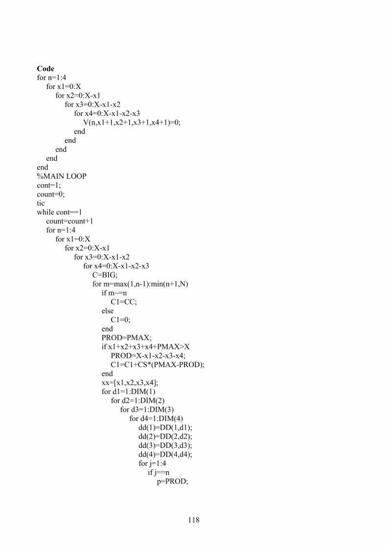
118

Code for n=1:4

for x1=0:X for x2=0:X-x1

for x3=0:X-x1-x2 for x4=0:X-x1-x2-x3

V(n,x1+1,x2+1,x3+1,x4+1)=0; end

end end

end end %MAIN LOOP cont=1; count=0; tic while cont==1

count=count+1 for n=1:4

for x1=0:X for x2=0:X-x1

for x3=0:X-x1-x2 for x4=0:X-x1-x2-x3

C=BIG; for m=max(1,n-1):min(n+1,N)

if m~=n C1=CC;

else C1=0;

end PROD=PMAX; if x1+x2+x3+x4+PMAX>X

PROD=X-x1-x2-x3-x4; C1=C1+CS*(PMAX-PROD);

end xx=[x1,x2,x3,x4]; for d1=1:DIM(1)

for d2=1:DIM(2) for d3=1:DIM(3)

for d4=1:DIM(4) dd(1)=DD(1,d1); dd(2)=DD(2,d2); dd(3)=DD(3,d3); dd(4)=DD(4,d4); for j=1:4

if j==n p=PROD;

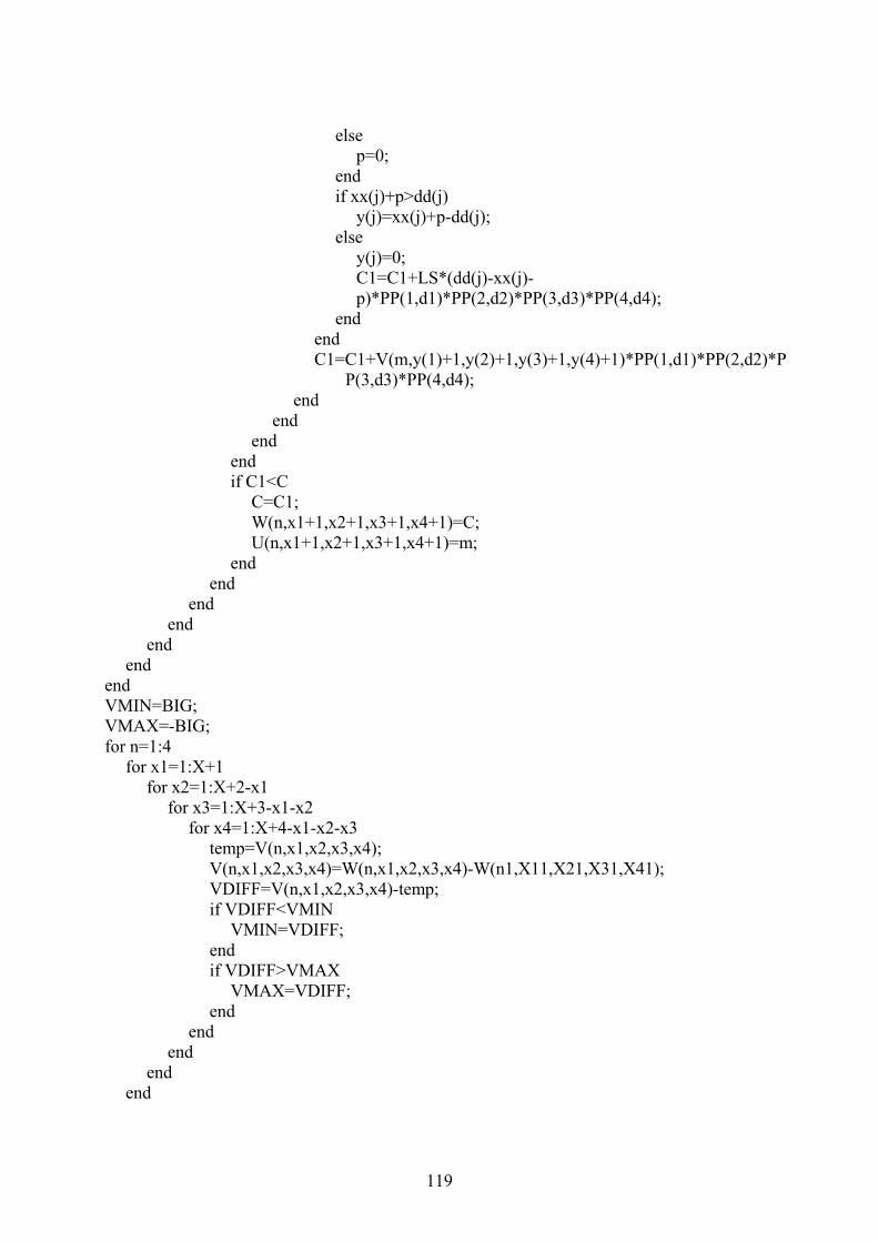
119

else p=0;

end if xx(j)+p>dd(j)

y(j)=xx(j)+p-dd(j); else

y(j)=0; C1=C1+LS*(dd(j)-xx(j)-p)*PP(1,d1)*PP(2,d2)*PP(3,d3)*PP(4,d4);

end end C1=C1+V(m,y(1)+1,y(2)+1,y(3)+1,y(4)+1)*PP(1,d1)*PP(2,d2)*P

P(3,d3)*PP(4,d4); end

end end

end if C1<C

C=C1; W(n,x1+1,x2+1,x3+1,x4+1)=C; U(n,x1+1,x2+1,x3+1,x4+1)=m;

end end

end end

end end

end VMIN=BIG; VMAX=-BIG; for n=1:4

for x1=1:X+1 for x2=1:X+2-x1

for x3=1:X+3-x1-x2 for x4=1:X+4-x1-x2-x3

temp=V(n,x1,x2,x3,x4); V(n,x1,x2,x3,x4)=W(n,x1,x2,x3,x4)-W(n1,X11,X21,X31,X41); VDIFF=V(n,x1,x2,x3,x4)-temp; if VDIFF<VMIN

VMIN=VDIFF; end if VDIFF>VMAX

VMAX=VDIFF; end

end end

end end

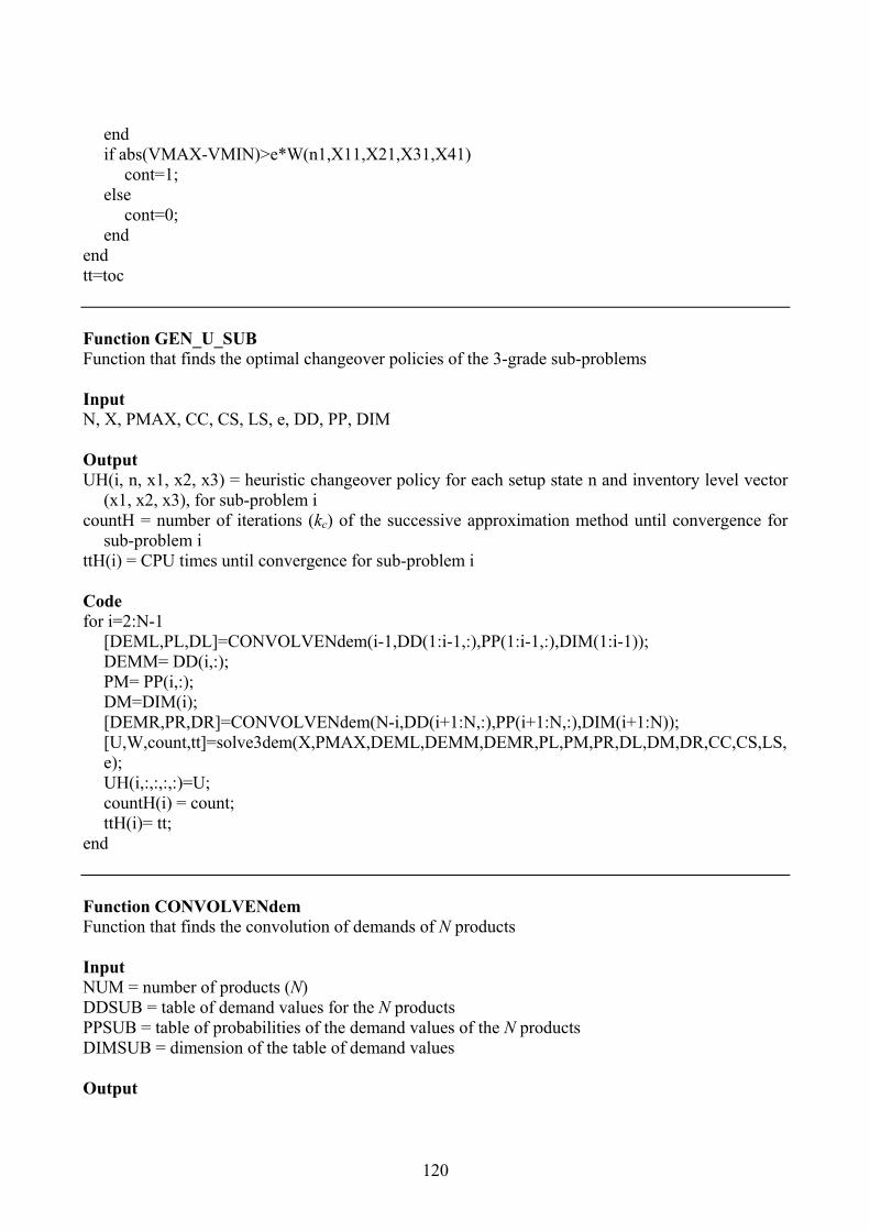
120

end if abs(VMAX-VMIN)>e*W(n1,X11,X21,X31,X41)

cont=1; else

cont=0; end

end tt=toc Function GEN_U_SUB Function that finds the optimal changeover policies of the 3-grade sub-problems Input N, X, PMAX, CC, CS, LS, e, DD, PP, DIM Output UH(i, n, x1, x2, x3) = heuristic changeover policy for each setup state n and inventory level vector

(x1, x2, x3), for sub-problem i countH = number of iterations (kc) of the successive approximation method until convergence for

sub-problem i ttH(i) = CPU times until convergence for sub-problem i Code for i=2:N-1

[DEML,PL,DL]=CONVOLVENdem(i-1,DD(1:i-1,:),PP(1:i-1,:),DIM(1:i-1)); DEMM= DD(i,:); PM= PP(i,:); DM=DIM(i); [DEMR,PR,DR]=CONVOLVENdem(N-i,DD(i+1:N,:),PP(i+1:N,:),DIM(i+1:N)); [U,W,count,tt]=solve3dem(X,PMAX,DEML,DEMM,DEMR,PL,PM,PR,DL,DM,DR,CC,CS,LS,e); UH(i,:,:,:,:)=U; countH(i) = count; ttH(i)= tt;

end Function CONVOLVENdem Function that finds the convolution of demands of N products Input NUM = number of products (N) DDSUB = table of demand values for the N products PPSUB = table of probabilities of the demand values of the N products DIMSUB = dimension of the table of demand values Output

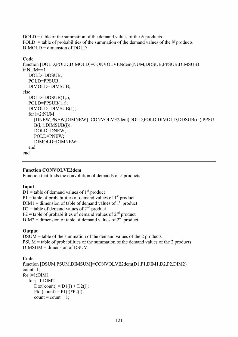
121

DOLD = table of the summation of the demand values of the N products POLD = table of probabilities of the summation of the demand values of the N products DIMOLD = dimension of DOLD Code function [DOLD,POLD,DIMOLD]=CONVOLVENdem(NUM,DDSUB,PPSUB,DIMSUB) if NUM==1

DOLD=DDSUB; POLD=PPSUB; DIMOLD=DIMSUB;

else DOLD=DDSUB(1,:); POLD=PPSUB(1,:); DIMOLD=DIMSUB(1); for i=2:NUM

[DNEW,PNEW,DIMNEW]=CONVOLVE2dem(DOLD,POLD,DIMOLD,DDSUB(i,:),PPSUB(i,:),DIMSUB(i)); DOLD=DNEW; POLD=PNEW; DIMOLD=DIMNEW;

end end Function CONVOLVE2dem Function that finds the convolution of demands of 2 products Input D1 = table of demand values of 1st product P1 = table of probabilities of demand values of 1st product DIM1 = dimension of table of demand values of 1st product D2 = table of demand values of 2nd product P2 = table of probabilities of demand values of 2nd product DIM2 = dimension of table of demand values of 2nd product Output DSUM = table of the summation of the demand values of the 2 products PSUM = table of probabilities of the summation of the demand values of the 2 products DIMSUM = dimension of DSUM Code function [DSUM,PSUM,DIMSUM]=CONVOLVE2dem(D1,P1,DIM1,D2,P2,DIM2) count=1; for i=1:DIM1

for j=1:DIM2 Dtot(count) = D1(i) + D2(j); Ptot(count) = P1(i)*P2(j); count = count + 1;

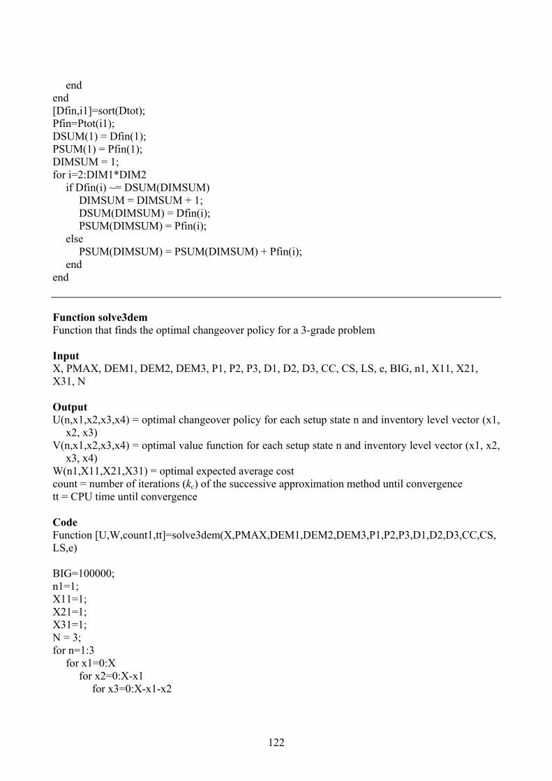
122

end end [Dfin,i1]=sort(Dtot); Pfin=Ptot(i1); DSUM(1) = Dfin(1); PSUM(1) = Pfin(1); DIMSUM = 1; for i=2:DIM1*DIM2

if Dfin(i) ~= DSUM(DIMSUM) DIMSUM = DIMSUM + 1; DSUM(DIMSUM) = Dfin(i); PSUM(DIMSUM) = Pfin(i);

else PSUM(DIMSUM) = PSUM(DIMSUM) + Pfin(i);

end end Function solve3dem Function that finds the optimal changeover policy for a 3-grade problem Input X, PMAX, DEM1, DEM2, DEM3, P1, P2, P3, D1, D2, D3, CC, CS, LS, e, BIG, n1, X11, X21, X31, N Output U(n,x1,x2,x3,x4) = optimal changeover policy for each setup state n and inventory level vector (x1,

x2, x3) V(n,x1,x2,x3,x4) = optimal value function for each setup state n and inventory level vector (x1, x2,

x3, x4) W(n1,X11,X21,X31) = optimal expected average cost count = number of iterations (kc) of the successive approximation method until convergence tt = CPU time until convergence Code Function [U,W,count1,tt]=solve3dem(X,PMAX,DEM1,DEM2,DEM3,P1,P2,P3,D1,D2,D3,CC,CS, LS,e) BIG=100000; n1=1; X11=1; X21=1; X31=1; N = 3; for n=1:3

for x1=0:X for x2=0:X-x1

for x3=0:X-x1-x2

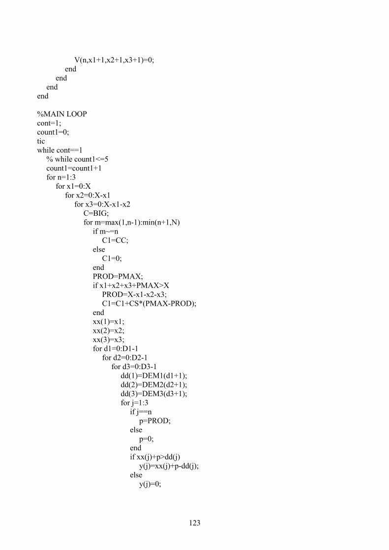
123

V(n,x1+1,x2+1,x3+1)=0; end

end end

end %MAIN LOOP cont=1; count1=0; tic while cont==1

% while count1<=5 count1=count1+1 for n=1:3

for x1=0:X for x2=0:X-x1

for x3=0:X-x1-x2 C=BIG; for m=max(1,n-1):min(n+1,N)

if m~=n C1=CC;

else C1=0;

end PROD=PMAX; if x1+x2+x3+PMAX>X

PROD=X-x1-x2-x3; C1=C1+CS*(PMAX-PROD);

end xx(1)=x1; xx(2)=x2; xx(3)=x3; for d1=0:D1-1

for d2=0:D2-1 for d3=0:D3-1

dd(1)=DEM1(d1+1); dd(2)=DEM2(d2+1); dd(3)=DEM3(d3+1); for j=1:3

if j==n p=PROD;

else p=0;

end if xx(j)+p>dd(j)

y(j)=xx(j)+p-dd(j); else

y(j)=0;

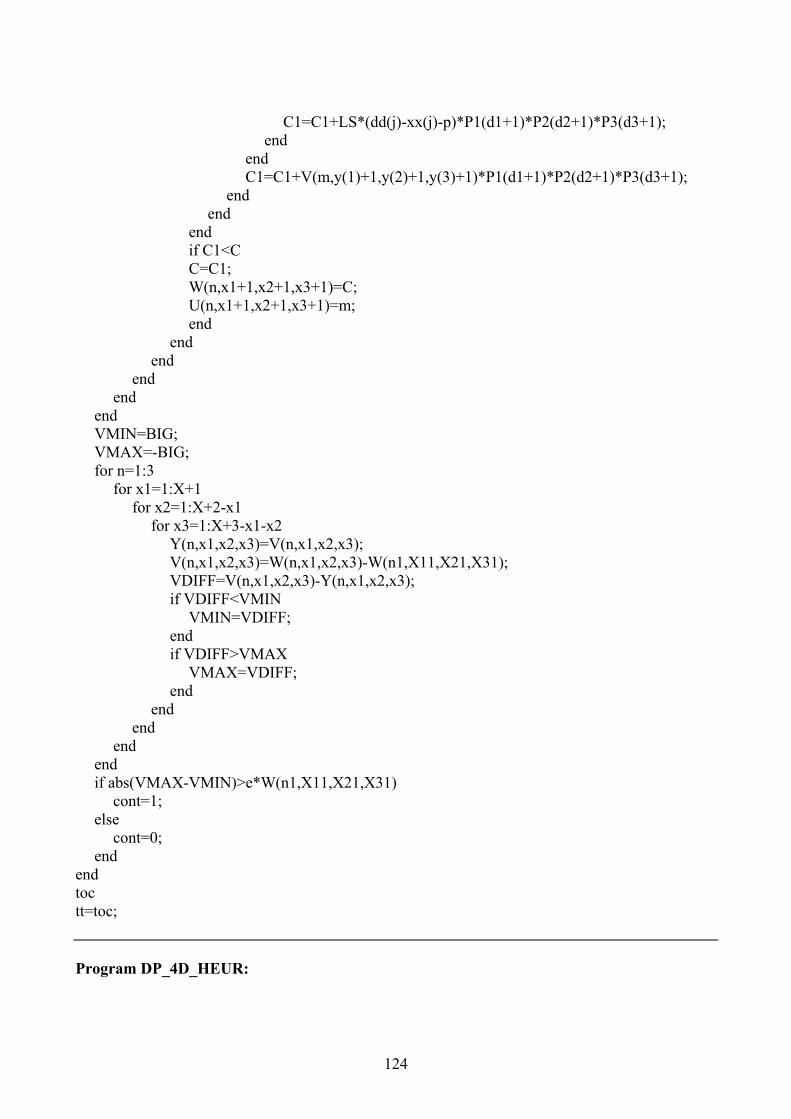
124

C1=C1+LS*(dd(j)-xx(j)-p)*P1(d1+1)*P2(d2+1)*P3(d3+1); end

end C1=C1+V(m,y(1)+1,y(2)+1,y(3)+1)*P1(d1+1)*P2(d2+1)*P3(d3+1);

end end

end if C1<C C=C1; W(n,x1+1,x2+1,x3+1)=C; U(n,x1+1,x2+1,x3+1)=m; end

end end

end end

end VMIN=BIG; VMAX=-BIG; for n=1:3

for x1=1:X+1 for x2=1:X+2-x1

for x3=1:X+3-x1-x2 Y(n,x1,x2,x3)=V(n,x1,x2,x3); V(n,x1,x2,x3)=W(n,x1,x2,x3)-W(n1,X11,X21,X31); VDIFF=V(n,x1,x2,x3)-Y(n,x1,x2,x3); if VDIFF<VMIN

VMIN=VDIFF; end if VDIFF>VMAX

VMAX=VDIFF; end

end end

end end if abs(VMAX-VMIN)>e*W(n1,X11,X21,X31)

cont=1; else

cont=0; end

end toc tt=toc; Program DP_4D_HEUR:

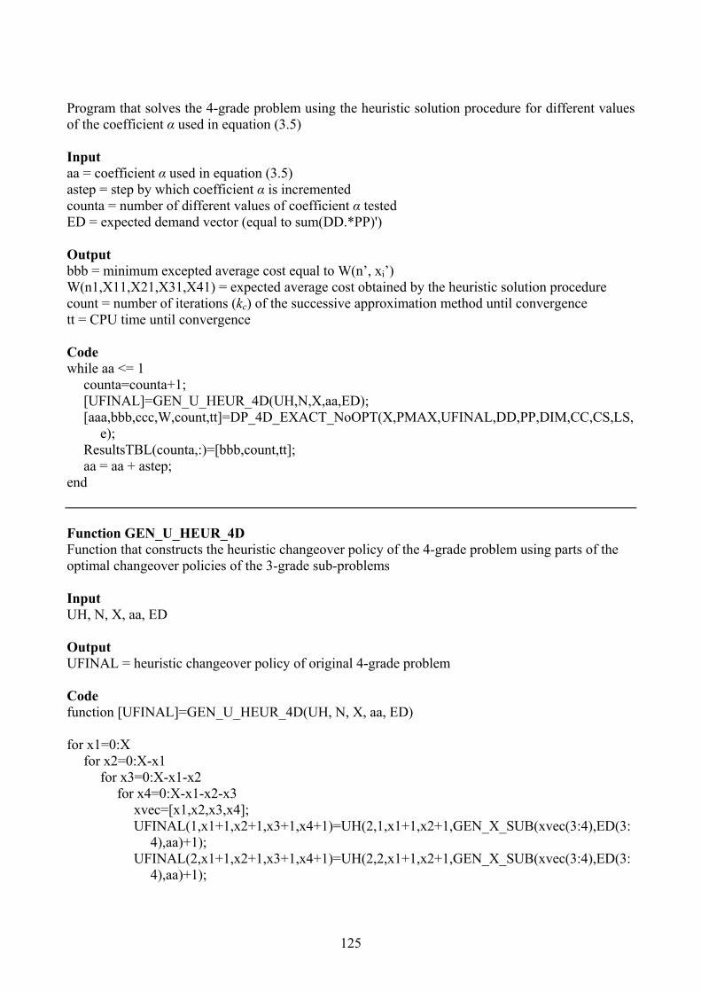
125

Program that solves the 4-grade problem using the heuristic solution procedure for different values of the coefficient α used in equation (3.5) Input aa = coefficient α used in equation (3.5) astep = step by which coefficient α is incremented counta = number of different values of coefficient α tested ED = expected demand vector (equal to sum(DD.*PP)') Output bbb = minimum excepted average cost equal to W(n’, xi’) W(n1,X11,X21,X31,X41) = expected average cost obtained by the heuristic solution procedure count = number of iterations (kc) of the successive approximation method until convergence tt = CPU time until convergence Code while aa <= 1

counta=counta+1; [UFINAL]=GEN_U_HEUR_4D(UH,N,X,aa,ED); [aaa,bbb,ccc,W,count,tt]=DP_4D_EXACT_NoOPT(X,PMAX,UFINAL,DD,PP,DIM,CC,CS,LS,

e); ResultsTBL(counta,:)=[bbb,count,tt]; aa = aa + astep;

end Function GEN_U_HEUR_4D Function that constructs the heuristic changeover policy of the 4-grade problem using parts of the optimal changeover policies of the 3-grade sub-problems Input UH, N, X, aa, ED Output UFINAL = heuristic changeover policy of original 4-grade problem Code function [UFINAL]=GEN_U_HEUR_4D(UH, N, X, aa, ED) for x1=0:X

for x2=0:X-x1 for x3=0:X-x1-x2

for x4=0:X-x1-x2-x3 xvec=[x1,x2,x3,x4]; UFINAL(1,x1+1,x2+1,x3+1,x4+1)=UH(2,1,x1+1,x2+1,GEN_X_SUB(xvec(3:4),ED(3:

4),aa)+1); UFINAL(2,x1+1,x2+1,x3+1,x4+1)=UH(2,2,x1+1,x2+1,GEN_X_SUB(xvec(3:4),ED(3:

4),aa)+1);

126

UFINAL(3,x1+1,x2+1,x3+1,x4+1)=UH(3,2,GEN_X_SUB(xvec(1:2),ED(1:2),aa)+1,x3+1,x4+1)+1;

UFINAL(4,x1+1,x2+1,x3+1,x4+1)=UH(3,3,GEN_X_SUB(xvec(1:2),ED(1:2),aa)+1,x3+1,x4+1)+1;

end end

end end Function GEN_X_SUB Function that calculates the inventory level of the aggregate product according to equation (3.5) Input x, ED, aa Output xnew = inventory level of the aggregate product Code function [xnew]=GEN_X_SUB(x,ED,aa) LS=sum(max(ED-x,0)); xnew=round((LS==0)*sum(x)+(LS>0)*(aa*(sum(ED)-LS)+(1-aa)*sum(x))); Function DP_4D_EXACT_NoOPT Function that evaluates the heuristic changeover policy of the 4-grade problem Input X, PMAX, U, DD, PP, CC, CS, LS, e, BIG, n1, X11, X21, X31, X41,DIM Output aaa = (VMAX-VMIN) bbb = W(n1,X11,X21,X31,X41) ccc = e* W(n1,X11,X21,X31,X41) W(n,x1,x2,x3,x4) = optimal value function mapping for each setup state n and inventory level

vector (x1, x2, x3, x4), given by equation (3.7) count = number of iterations (kc) of the successive approximation method until convergence tt = CPU time until convergence Code function [aaa,bbb,ccc,W,count,tt]=DP_4D_EXACT_NoOPT(X,PMAX,U,DD,PP,DIM,CC,CS,LS,e); for n=1:4

for x1=0:X for x2=0:X-x1

for x3=0:X-x1-x2 for x4=0:X-x1-x2-x3

127

V(n,x1+1,x2+1,x3+1,x4+1)=0; end

end end

end end %MAIN LOOP cont=1; count=0; tic while cont==1

% while count==0 count=count+1 for n=1:4

for x1=0:X for x2=0:X-x1

for x3=0:X-x1-x2 for x4=0:X-x1-x2-x3

m=U(n,x1+1,x2+1,x3+1,x4+1); if m~=n

C1=CC; else

C1=0; end PROD=PMAX; if x1+x2+x3+x4+PMAX>X

PROD=X-x1-x2-x3-x4; C1=C1+CS*(PMAX-PROD);

end xx=[x1,x2,x3,x4]; for d1=1:DIM(1)

for d2=1:DIM(2) for d3=1:DIM(3)

for d4=1:DIM(4) dd(1)=DD(1,d1); dd(2)=DD(2,d2); dd(3)=DD(3,d3); dd(4)=DD(4,d4); for j=1:4

if j==n p=PROD;

else p=0;

end if xx(j)+p>dd(j)

y(j)=xx(j)+p-dd(j); else

128

y(j)=0; C1=C1+LS*(dd(j)-xx(j)-p)*PP(1,d1)*PP(2,d2)*PP(3,d3)*

PP(4,d4); end

end C1=C1+V(m,y(1)+1,y(2)+1,y(3)+1,y(4)+1)*PP(1,d1)*PP(2,d2)*PP(3,

d3)*PP(4,d4); end

end end

end W(n,x1+1,x2+1,x3+1,x4+1)=C1;

end end

end end

end VMIN=BIG; VMAX=-BIG; for n=1:4

for x1=1:X+1 for x2=1:X+2-x1

for x3=1:X+3-x1-x2 for x4=1:X+4-x1-x2-x3

temp=V(n,x1,x2,x3,x4); V(n,x1,x2,x3,x4)=W(n,x1,x2,x3,x4)-W(n1,X11,X21,X31,X41); VDIFF=V(n,x1,x2,x3,x4)-temp; if VDIFF<VMIN

VMIN=VDIFF; end if VDIFF>VMAX

VMAX=VDIFF; end

end end

end end

end if abs(VMAX-VMIN)>e*W(n1,X11,X21,X31,X41) cont=1; else cont=0; end

end tt=toc Program SIM_4D_EXACT

129

Program that evaluates the optimal changeover policy of the 4-grade problem using simulation Input Ν, X, PMAX, CC, CS, LS, e, DD, PP, DIM,U Output CTOT = total cost tsim = simulation time Code load('DP_4D_1_EXACT.mat','U'); load('DATA_4D_1.mat'); R = 60; T = 100000; Ccum=0; Csqcum=0; tcum=0; CCI=0; for i=1:R

[CTOT,tsim]=SIM_4D(X,PMAX,U,DD,PP,DIM,CC,CS,LS,N,T); CTOTMAT(i)=CTOT; TSIMMAT(i)=tsim; Ccum=Ccum+CTOT; Csqcum = Csqcum + CTOT^2; tcum=tcum+tsim;

end Program SIM_4D_HEUR Program that evaluates the heuristic changeover policy of the 4-grade problem for different values of the coefficient α used in equation (3.5), using simulation Input X, PMAX, UFINAL, DD, PP, DIM, CC, CS, LS, N, astep, aa, counta, ED T = total number of counts in simulation R = demand width U_SUB = sub-problem policies Output Caver = average total cost CConfInter = confidence interval of average total cost taver = average total CPU time until a solution is reached through simulation Code while aa <=1

counta=counta+1; [UFINAL]=GEN_U_HEUR_4D(UH,N,X,aa,ED); Ccum=0;

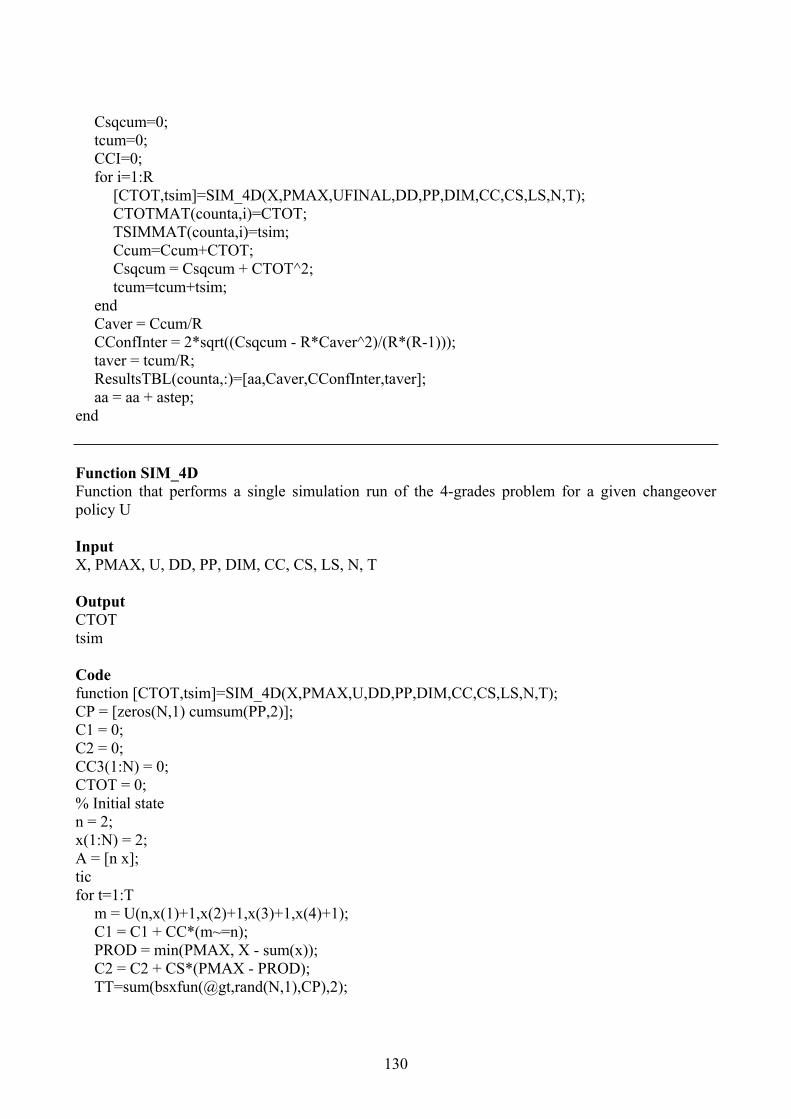
130

Csqcum=0; tcum=0; CCI=0; for i=1:R

[CTOT,tsim]=SIM_4D(X,PMAX,UFINAL,DD,PP,DIM,CC,CS,LS,N,T); CTOTMAT(counta,i)=CTOT; TSIMMAT(counta,i)=tsim; Ccum=Ccum+CTOT; Csqcum = Csqcum + CTOT^2; tcum=tcum+tsim;

end Caver = Ccum/R CConfInter = 2*sqrt((Csqcum - R*Caver^2)/(R*(R-1))); taver = tcum/R; ResultsTBL(counta,:)=[aa,Caver,CConfInter,taver]; aa = aa + astep;

end Function SIM_4D Function that performs a single simulation run of the 4-grades problem for a given changeover policy U Input X, PMAX, U, DD, PP, DIM, CC, CS, LS, N, T Output CTOT tsim Code function [CTOT,tsim]=SIM_4D(X,PMAX,U,DD,PP,DIM,CC,CS,LS,N,T); CP = [zeros(N,1) cumsum(PP,2)]; C1 = 0; C2 = 0; CC3(1:N) = 0; CTOT = 0; % Initial state n = 2; x(1:N) = 2; A = [n x]; tic for t=1:T

m = U(n,x(1)+1,x(2)+1,x(3)+1,x(4)+1); C1 = C1 + CC*(m~=n); PROD = min(PMAX, X - sum(x)); C2 = C2 + CS*(PMAX - PROD); TT=sum(bsxfun(@gt,rand(N,1),CP),2);

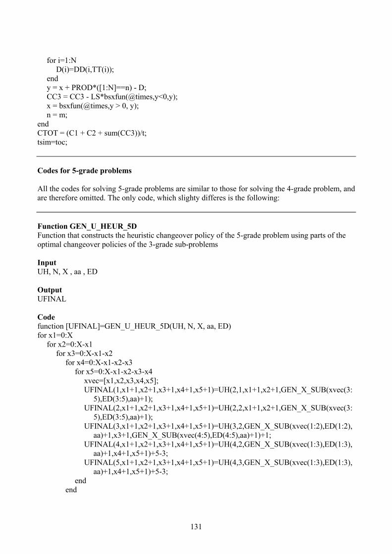
131

for i=1:N D(i)=DD(i,TT(i));

end y = x + PROD*([1:N]==n) - D; CC3 = CC3 - LS*bsxfun(@times,y<0,y); x = bsxfun(@times,y > 0, y); n = m;

end CTOT = (C1 + C2 + sum(CC3))/t; tsim=toc; Codes for 5-grade problems All the codes for solving 5-grade problems are similar to those for solving the 4-grade problem, and are therefore omitted. The only code, which slighty differes is the following: Function GEN_U_HEUR_5D Function that constructs the heuristic changeover policy of the 5-grade problem using parts of the optimal changeover policies of the 3-grade sub-problems Input UH, N, X , aa , ED Output UFINAL Code function [UFINAL]=GEN_U_HEUR_5D(UH, N, X, aa, ED) for x1=0:X

for x2=0:X-x1 for x3=0:X-x1-x2

for x4=0:X-x1-x2-x3 for x5=0:X-x1-x2-x3-x4

xvec=[x1,x2,x3,x4,x5]; UFINAL(1,x1+1,x2+1,x3+1,x4+1,x5+1)=UH(2,1,x1+1,x2+1,GEN_X_SUB(xvec(3:

5),ED(3:5),aa)+1); UFINAL(2,x1+1,x2+1,x3+1,x4+1,x5+1)=UH(2,2,x1+1,x2+1,GEN_X_SUB(xvec(3:

5),ED(3:5),aa)+1); UFINAL(3,x1+1,x2+1,x3+1,x4+1,x5+1)=UH(3,2,GEN_X_SUB(xvec(1:2),ED(1:2),

aa)+1,x3+1,GEN_X_SUB(xvec(4:5),ED(4:5),aa)+1)+1; UFINAL(4,x1+1,x2+1,x3+1,x4+1,x5+1)=UH(4,2,GEN_X_SUB(xvec(1:3),ED(1:3),

aa)+1,x4+1,x5+1)+5-3; UFINAL(5,x1+1,x2+1,x3+1,x4+1,x5+1)=UH(4,3,GEN_X_SUB(xvec(1:3),ED(1:3),

aa)+1,x4+1,x5+1)+5-3; end

end

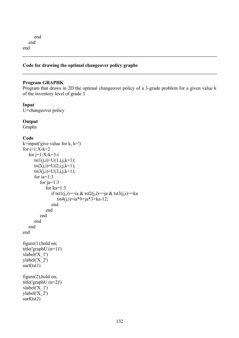
132

end end

end Code for drawing the optimal changeover policy graphs Program GRAPHK Program that draws in 2D the optimal changeover policy of a 3-grade problem for a given value k of the inventory level of grade 3 Input U=changeover policy Output Graphs Code k=input('give value for k, k=') for i=1:X-k+2

for j=1:X-k+3-i tst1(j,i)=U(1,i,j,k+1); tst2(j,i)=U(2,i,j,k+1); tst3(j,i)=U(3,i,j,k+1); for ia=1:3

for ja=1:3 for ka=1:3

if tst1(j,i)==ia & tst2(j,i)==ja & tst3(j,i)==ka tst4(j,i)=ia*9+ja*3+ka-12;

end end

end end

end end figure(1);hold on; title('graphU (n=1)') xlabel('X_1') ylabel('X_2') surf(tst1) figure(2);hold on; title('graphU (n=2)') xlabel('X_1') ylabel('X_2') surf(tst2)

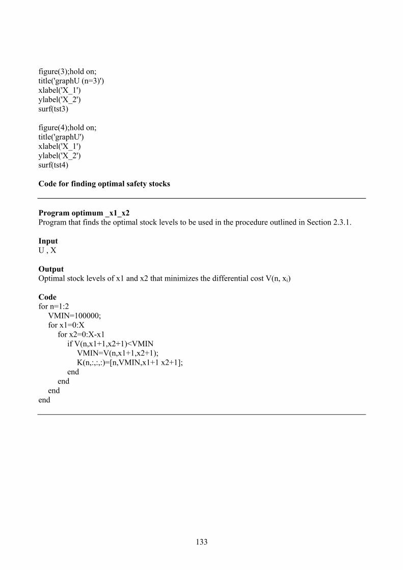
133

figure(3);hold on; title('graphU (n=3)') xlabel('X_1') ylabel('X_2') surf(tst3) figure(4);hold on; title('graphU') xlabel('X_1') ylabel('X_2') surf(tst4) Code for finding optimal safety stocks Program optimum _x1_x2 Program that finds the optimal stock levels to be used in the procedure outlined in Section 2.3.1. Input U , Χ Output Optimal stock levels of x1 and x2 that minimizes the differential cost V(n, xi) Code for n=1:2

VMIN=100000; for x1=0:X

for x2=0:X-x1 if V(n,x1+1,x2+1)<VMIN

VMIN=V(n,x1+1,x2+1); K(n,:,:,:)=[n,VMIN,x1+1 x2+1];

end end

end end

134

135

Appendix E: Results of the heuristic policy evaluated in

Section 3.4.3 for different values of parameter α

Table A-3. Complete set of results of the heuristic policy evaluated using the value iteration method

for the 4-grade example presented in Section 3.4.3

Case Demandpattern

CPU (sec) a kc Jh(a)

44308 0 70 1.389142126 0.1 69 1.375125188 0.2 68 1.386731836 0.3 60 1.364230887 0.4 57 1.317129465 0.5 56 1.290419948 0.6 55 1.2566

1 B,D,D,B

69925 0.7 130 1.244235192 0 146 1.236731127 0.1 156 1.230533289 0.2 166 1.228534647 0.3 172 1.226934960 0.4 175 1.226335096 0.5 175 1.225334571 0.6 173 1.2267

2 D,D,B,B

33754 0.7 169 1.227140549 0 203 1.231271143 0.1 355 1.232876778 0.2 215 1.3262126720 0.3 211 1.331120180 0.4 206 1.329174241 0.5 202 1.3314103620 0.6 195 1.3376

3 D,B,D,B

67907 0.7 191 1.338860305 0 115 1.314141770 0.1 118 1.313988204 0.2 118 1.314241296 0.3 117 1.315661512 0.4 117 1.315969141 0.5 116 1.316471163 0.6 115 1.3168

4 D,B,B,D

40356 0.7 115 1.3172

136

Table A-4. Complete set of results of the heuristic policy evaluated using simulation for the 4-grade

example presented in Section 3.4.3

Case Demandpattern

CPU (sec) a Jh(a) (95% c.i.)

12.617 0 1.3359±0.001412.593 0.1 1.3206±0.001912.788 0.2 1.3272±0.001912.639 0.3 1.3253±0.002112.797 0.4 1.3303±0.001712.835 0.5 1.3321±0.001713.096 0.6 1.3367±0.001612.832 0.7 1.3384±0.002112.632 0.8 1.3385±0.001812.582 0.9 1.3421±0.0016

1 B,D,D,B

12.443 1 1.3416±0.002111.182 0 1.3140±0.002111.117 0.1 1.3135±0.001811.047 0.2 1.3144±0.001311.031 0.3 1.3157±0.001611.033 0.4 1.3159±0.002011.031 0.5 1.3170±0.001711.030 0.6 1.3172±0.001811.026 0.7 1.3179±0.001811.032 0.8 1.3183±0.002011.038 0.9 1.3174±0.0017

2 D,D,B,B

11.035 1 1.3181±0.00216.475 0 1.3898±0.00226.482 0.1 1.3761±0.00216.484 0.2 1.3867±0.00246.547 0.3 1.3599±0.00226.475 0.4 1.3178±0.00146.503 0.5 1.2894±0.00216.529 0.6 1.2564±0.00156.484 0.7 1.2445±0.00196.476 0.8 1.2719±0.01536.489 0.9 2.7741±0.5626

3 D,B,D,B

6.483 1 2.8880±0.52448.6171 0 1.2356±0.00118.5913 0.1 1.2308±0.00108.6226 0.2 1.2288±0.00118.5926 0.3 1.2265±0.00118.4072 0.4 1.2263±0.0010

4 D,B,B,D

8.3407 0.5 1.2253±0.0011

137

8.3839 0.6 1.2276±0.00108.3947 0.7 1.2268±0.00108.3795 0.8 1.2305±0.00108.3666 0.9 1.2328±0.00098.3711 1 1.3153±0.0296

Table A-5. Complete set of results of the heuristic policy evaluated using simulation for the 5-grade

example presented in Section 3.4.3

Case Demand pattern

CPU (sec) a Jh(a) (95% c.i.)

3.8711 0 3.1001±0.00163.8590 0.1 3.0355±0.00163.8558 0.2 3.0800±0.00203.8533 0.3 3.1530±0.00203.8600 0.4 3.2087±0.00253.8538 0.5 3.3301±0.00253.8432 0.6 3.6575±0.00293.8422 0.7 5.4469±0.00363.8425 0.8 5.4512±0.00333.8420 0.9 5.4227±0.0034

1 A,C,D,C,A

3.8428 1 5.4595±0.00313.8840 0 3.4926±0.00173.8500 0.1 3.4512±0.00153.8622 0.2 3.4644±0.00203.8242 0.3 3.4641±0.00183.8852 0.4 3.4578±0.00163.8335 0.5 3.4852±0.00193.8244 0.6 3.5318±0.00304.1222 0.7 3.8665±0.01284.0414 0.8 5.6717±0.02913.8489 0.9 8.2742±0.0027

2 D,C,C,A,A

3.8103 1 8.2735±0.00293.6524 0 3.8759±0.00203.1777 0.1 3.9863±0.00182.7754 0.2 4.0763±0.00282.2716 0.3 4.2347±0.00272.2910 0.4 4.3579±0.00312.2859 0.5 4.5680±0.00452.3008 0.6 4.8012±0.00492.2945 0.7 5.2577±0.00582.2896 0.8 7.3457±0.00552.2916 0.9 10.3628±0.0030

3 D,C,A,A,C

2.2757 1 10.3631±0.00264 D,A,C,A,C 3.7605 0 3.9348±0.0020

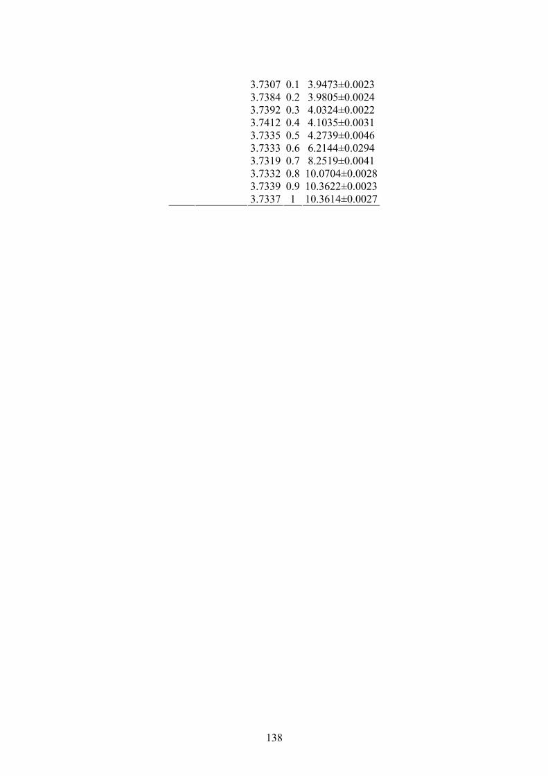
138

3.7307 0.1 3.9473±0.00233.7384 0.2 3.9805±0.00243.7392 0.3 4.0324±0.00223.7412 0.4 4.1035±0.00313.7335 0.5 4.2739±0.00463.7333 0.6 6.2144±0.02943.7319 0.7 8.2519±0.00413.7332 0.8 10.0704±0.00283.7339 0.9 10.3622±0.00233.7337 1 10.3614±0.0027